Studying the Optimal Frequency Control Condition for Electric Vehicle Fast Charging Stations as a Dynamic Load Using Reinforcement Learning Algorithms in Different Photovoltaic Penetration Levels

Abstract

This study investigates the impact of renewable energy penetration on system stability and validates the performance of the (Proportional-Integral-Derivative) PID-(reinforcement learning) RL control technique. Three scenarios were examined: no photovoltaic (PV), 25% PV, and 50% PV, to evaluate the impact of PV penetration on system stability. The results demonstrate that while the absence of renewable energy yields a more stable frequency response, a higher PV penetration (50%) enhances stability in tie-line active power flow between interconnected systems. This shows that an increased PV penetration improves frequency balance and active power flow stability. Additionally, the study evaluates three control scenarios: no control input, PID-(Particle Swarm Optimization) PSO, and PID-RL, to validate the performance of the PID-RL control technique. The findings show that the EV system with PID-RL outperforms the other scenarios in terms of frequency response, tie-line active power response, and frequency difference response. The PID-RL controller significantly enhances the damping of the dominant oscillation mode and restores the stability within the first 4 s—after the disturbance in first second. This leads to an improved stability compared to the EV system with PID-PSO (within 21 s) and without any control input (oscillating more than 30 s). Overall, this research provides the improvement in terms of frequency response, tie-line active power response, and frequency difference response with high renewable energy penetration levels and the research validates the effectiveness of the PID-RL control technique in stabilizing the EV system. These findings can contribute to the development of strategies for integrating renewable energy sources and optimizing control systems, ensuring a more stable and sustainable power grid.

1. Introduction

The power system is facing major changes and challenges as a result of the growing integration of renewable energy sources and the rising popularity of electric vehicles (EVs). It becomes increasingly important to ensure system stability as the penetration of renewable energy increases. Furthermore, the rapid expansion of EVs calls for a dependable and effective infrastructure for charging them, which calls for efficient frequency control. Thus, the goal of this research is to determine the best scenario for a dynamic load in frequency regulation for electric vehicle fast charging stations by utilizing a reinforcement learning (RL) algorithm and renewable energy penetration [1,2,3]. There are several environmental and financial advantages to using renewable energy sources, such as wind and solar energy [2,4,5]. Figure 1 shows the percentage of CO₂ emissions attributable to different sectors: industry, transportation, residential, electricity and heat, and other sectors worldwide [6].

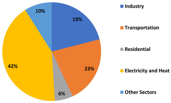
Figure 1. The percentage of world CO₂ emissions attributable to each sector (IEA, 2016) [6] Source: IEA/OECD CO₂ emissions from fuel combustion, 2016.

The renewable sources’ intermittency makes it difficult to keep the system stable because variations in generation might cause frequency variances. Therefore, it is crucial to investigate how the penetration of renewable energy affects the system’s stability and to create plans to address any possible problems [5,7]. Furthermore, the widespread use of EVs has increased the demand for infrastructure related to charging. In order to meet the changing requirements of electric vehicles (EVs), provide user convenience, and encourage the wider use of electric mobility, fast charging stations are essential. When there is a significant demand for EV charging, efficient frequency control is essential for controlling the charging load and preserving grid stability [8,9,10,11,12,13].

The increasing integration of renewable energy sources and the massive growth of EVs are transforming the global energy landscape as shown in Figure 2. Renewable energy sources, like wind and solar energy, provide sustainable and environmentally friendly substitutes for conventional fossil fuel-based power. The broad deployment of EVs intends to lessen the transportation sector’s reliance on fossil fuels and greenhouse gas emissions at the same time. These advancements, nonetheless, provide new difficulties for the power system and call for creative fixes to guarantee grid stability and effective infrastructure for charging [14,15,16].

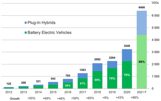
Figure 2. The global electric vehicle growth [13].

Although it is much desired, intermittent generation is produced by renewable energy sources because they are weather-dependent. The power grid may experience frequency fluctuations as a result of the fluctuating output of renewable energy, which could jeopardize system stability. For power systems to function dependably, a steady frequency must be maintained because fluctuations might affect linked equipment’s performance and upset the supply and demand balance. Thus, it is crucial to comprehend how the penetration of renewable energy affects system stability in order to guarantee the dependable integration of clean energy sources. Furthermore, a reliable and effective charging infrastructure is now required due to the rising popularity of EVs. Long-distance driving and reduced charging times for EV users are made possible by EV fast charging stations, which are essential in satisfying the growing demand for quick charging. Nevertheless, these fast charging stations’ high power requirements can put pressure on the grid, causing variations in frequency and voltage. During times of heavy demand for EV charging, efficient frequency control is crucial to managing the charging load and maintaining grid stability [17,18,19,20].

2. Related Works

A secondary controller was created and used in [21] to control the system frequency in a networked microgrid system. Energy-storing units (ESUs), synchronous generators, and renewable energy resources (RESs) made up the suggested power system. Photovoltaic (PV) and wind turbine generator (WTG) units are two examples of renewable energy sources. A flywheel and a battery made up the ESU. Despite various load demand variations and renewable energy sources, the deployed (Mayfly Algorithm) MA-PID controller proved its ability to deliver and control the system frequency effectively. The study’s validation comparisons provided verification of this [21].

A novel form of power system surfaced as a means of fulfilling China’s carbon emission reduction objectives for the years 2030 and 2060. One of the most significant challenges facing this field of technical innovation is coordinating the energy storage systems (ESSs), load, network infrastructures, and generation. It is necessary to estimate the associated static and dynamic model parameters accurately and effectively in order to manage and run these grid resources in a secure, reliable, and cost-effective manner. Power systems have made use of deep reinforcement learning (DRL), a popular artificial intelligence technique in recent years, especially in control-related domains. DRL is a potent optimization tool that produces promising results when used to solve parameter estimate issues. As a result, the DRL techniques used to estimate the parameters of power system models, including load and generator models, were thoroughly addressed in this study [22].

When compared to synchronous generation power grids, inverter-based networks are not physically able to produce a substantial amount of inertia. This calls for greater in-depth research on stability issues related to these kinds of systems. Consequently, in power systems with significant penetration rates of renewable energy, when many inverters and dispersed energy sources are involved, it is imperative to utilize suitable analytical techniques for voltage stability analysis. This study reviewed the literature in-depth on voltage stability analyses in power systems that include a significant amount of renewable energy. There was a discussion of several upgrade techniques and assessment plans for voltage stability in power networks with various distributed energy sources. The study also conducted a thorough examination of the simulation verification models and voltage stability analysis techniques currently in use for microgrids. The many distributed generator types, microgrid designs, and modes of operation were taken into consideration when reviewing the conventional and enhanced voltage stability analysis methods. Furthermore, a detailed evaluation of the voltage stability indices was conducted, taking into account the applicable conditions. These indices are crucial in voltage stability assessments [23].

The goal of the project was to model a fleet of EVs in order to offer Frequency Containment Reserve for Disturbance (FCR-D) upwards and Firm Frequency Response (FFR) services while adhering to current laws and regulations. The Nordic 45 test model (N45) is an enhanced version of the Nordic 44 test model (N44) that was created to perform more accurate simulations of the Nordic power system. To evaluate various aspects of electric vehicle (EV) performance as frequency reserve providers in Kundur’s two-area power system model (K2A) and the new N45 test model, ten simulation cases were developed. After presenting and analyzing the simulation findings, a conclusion about the viability of EVs as frequency reserve suppliers in the current Nordic power system was reached. Because EV charging equipment and measurement devices have an inherent time delay, it was found that deploying EVs for FCR-D and FFR services was not currently possible. However, it was found that the usefulness of using EVs as frequency reserve providers might be improved if the time delay of these components was much lowered, enabling nearly instantaneous activation of EVs’ frequency response following a fault occurrence [24].

Reference [25] presented a two-stage transfer and deep learning-based method to predict dynamic frequency in power systems after disturbances and find the best event-based load-shedding plan to keep the frequency of the system stable. Convolutional Neural Networks (CNNs) and Long Short-Term Memory (LSTM) networks were coupled in the suggested method to efficiently use the input data’s spatial and temporal measurements. The CNN-LSTM technique greatly improved the timeliness of online frequency control while maintaining good accuracy and efficacy, according to simulation findings performed on the IEEE 118-bus system. Furthermore, test cases conducted on the South Carolina 500-bus system and the New England 39-bus system showed that the transfer learning procedure produced accurate results even in the presence of a shortage of training data [25].

Another study proposed a system to enable a thorough examination of grid transient stability, based on several machine-learning algorithms. Furthermore, the framework made it easier to thoroughly identify new patterns that appeared in the dynamic response of individual synchronous generators in systems with reduced inertia. Given that crucial operating points fluctuate in systems with high renewable penetration, the framework’s capacity to evaluate all hourly operating points over the course of a study year was a significant advantage. An IEEE-39 system was used as a case study, integrating inverter-based resources at different penetration levels and locations, to illustrate the advantages of the suggested platform [26].

The literature assessment indicates that further research and exploration of the optimal condition as a reinforcement learning algorithm for electric vehicle fast charging stations and a dynamic load for frequency control using renewable energy integration is still possible. To overcome these obstacles and achieve optimal frequency regulation and effective operation of fast charging stations, this research suggests using a reinforcement learning (RL) algorithm in conjunction with renewable energy penetration. Because RL algorithms may learn optimal control policies through interactions with the environment, they are especially well suited for dynamic and unpredictable systems, such as electric grids and networks for electric vehicle charging. There are two goals that this study aims to achieve. First, in order to evaluate the effect of renewable energy penetration on system stability, it looks at the frequency response and active power flow under various photovoltaic (PV) penetration scenarios. Second, it endeavors to assess how well the suggested RL algorithm performs in terms of attaining optimal frequency control and guaranteeing the efficient operation of EV fast charging stations.

After the introduction and the related work in Section 1 and Section 2, respectively, the rest of this article has been designed as follows: Section 3 describes the proposed methodology and it covers system identifications and simulation tools as well as the mathematical model of EV charging stations. In addition, Section 3 describes the development of merging traditional PID control with RL using the adaptive PID controller and Q-learning. In Section 4, the experimental setup and Kundur’s model details have been explained. The analysis of case studies as well as the results have been highlighted in Section 5. Finally, Section 6 and Section 7 cover the discussion and conclusion of this research including the main findings and future work.

3. Methodology

This section introduces the methodology of this research. It involves a Proportional-Integral-Derivative (PID) controller, reinforcement learning (RL), design-adaptive PID controller using Quality (Q)-learning, and experimental setup.

The increasing integration of renewable energy sources in today’s modern power systems creates an urgent need to address the decreasing system inertia [1]. A potential solution to this problem is to combine RL techniques with the conventional Proportional-Integral-Derivative (PID) control as seen in Figure 3. Power system operators face a distinct set of issues when integrating renewable energy sources. Variations in power generation are caused by the intrinsic variability and uncertainty of renewable sources, which distinguishes them from conventional power plants. As a result, the overall inertia of the system tends to diminish, which is important for maintaining stability. It is crucial to use reinforcement learning approaches to improve the performance of current control mechanisms, like PID control, in order to overcome this deterioration.

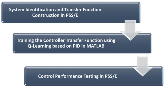
Figure 3. Stages of controller design.

Therefore, in order to preserve power system stability during the integration of renewable energy sources, creative control measures are required. Through the integration of PID control and reinforcement learning, the control system can be made more capable of responding to changing circumstances and improving overall system performance. The evaluation results show this approach’s efficacy and highlight its potential for a range of power system applications. Subsequent investigations may concentrate on enhancing the control approach and investigating supplementary prospects for its integration into practical power systems.

The Power System Simulation for Engineering (PSS/E) is used to model the power system with great care from the beginning of the design process. Dynamic equations relevant to the control actuator (a governor or a power electronic converter) are generated within this framework. The transfer function is then trained using the model-free RL algorithm known as Q-learning. The first step in this process is to define the actions, the state space, and a reward function that are all carefully customized for the power system.

The final phase is to validate the developed controller in multiple PSS/E scenarios. After being fitted with PID parameters that are taken out of the Q-learning procedure, the controller is tested to determine how reliable and effective it is. The primary goal is to make sure that the controller improves the power system’s general stability and reliability while simultaneously mitigating the difficulties brought on by significant renewable integration.

3.1. System Identification and Transfer Function Construction in PSS/E

A popular software program for power system analysis is called PSS/E. Techniques for system identification are used to collect information and examine how the system reacts to various inputs or disruptions. The transfer function of the system, which depicts the connection between its input and output, is then estimated using this data.

In order to construct a mathematical model, system identification involves creating a dynamic system representation using measurement data. Three crucial processes are included in the model development process, which is based on the following measurements [2]:

Stage 1: input–output selection: this refers to choosing the best actuation and observation signals.

Stage 2: system identification: building the functional model is the task of this step.

Stage 3: controller design: this entails creating a controller using the system that has been identified.

Initially, a set of differential equations called the subspace state-space model or difference equations are used to generate a transfer function model [3]. Then, using system identification techniques, a model is created based on real measurements [4].

The measurement-guided model structure makes use of the Output Error (OE) polynomial model. Within the category of polynomial models, this model is a particular configuration that is used, in this case, for model identification using probing measurements. Conventional transfer functions are described by means of OE models, in which the system is defined by the combined effects of the measured outputs and the inputs (represented by injected noise) [5].

Figure 3 shows the simulated response comparison between validation data (y_1) and model_OE 94.02 %. Amplitude per time can be obtained according to Figure 4.

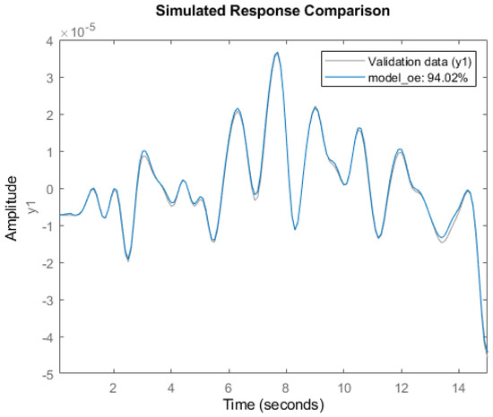
Figure 4. Transfer function validation.

The system structure can be described as follows, assuming that the injected noise signal has enough information to identify a system model with the chosen order of n as Equation (1) [7]:

$$y(k)=\frac{B(z,\theta )}{F(z,\theta )}u(k)+e(k)=\frac{b_1{z}^{-1}+\cdots +b_n{z}^z\cdot n_b}{1+f_1{z}^{-1}+\cdots +f_n{z}^{-n}}u(k)+e(k)$$

(1)

The OE mathematical model is therefore represented by Equation (2):

$$\overline{y}(t)+\sum _{k=1}^n a_k\overline{y}(t-k)=\sum _{j=1}^n b_{j}u(t-j)+e(t)$$

(2)

where t denotes the sampled data index, e represents the injected noise process, u and $\overline{y}$ are the input and output of the model, $a_k$ is the model coefficient denominator, and $b_j$ is the model coefficient numerator.

For time-domain validation, the created model and the real model responses are compared. To achieve fit accuracy between the created system and the real model response, the original data that was used to build the model must be available. This is known as the actual system response. Equation (3) is used to express how accurate the system that was built is [8] and is as follows:

$$\mathrm{Accuracy} \mathrm{Index} =\left(1-\frac{∥Y_i-{\widehat{Y}}_i∥}{∥Y_i-{\overline{Y}}_i∥}\right)\times 100$$

(3)

where $Y_i$ and ${\widehat{Y}}_i$ denote the constructed model and actual system responses, respectively, and ${\widehat{Y}}_i$ is the mean of the actual system response over several periods. The index should approach 1, indicating that the constructed model response aptly represents the actual system.

3.2. Mathematical Computations and Analysis of Aggregated Electric Vehicles for Frequency Regulation

To use EVs in frequency regulation, multiple EVs must be connected to the power grid. An EV aggregator is an EV control center that manages the battery charge and discharge behavior of all EVs in the aggregator. The dynamic model of the ith EV in the EV aggregator is presented by the first-order transfer function as in Equation (4):

$${\mathrm{G}}_{\mathrm{E}\mathrm{V}}=\frac{{\mathrm{K}}_{\mathrm{E}\mathrm{V}}}{\mathrm{S}{\mathrm{T}}_{\mathrm{E}\mathrm{V}}+1}$$

(4)

where K_EV and T_EV are the gain and time constants of the ith EV battery system, respectively.

The transfer function of $e^{-s{\rho }_i}$ is used to describe the communication delay from an EV aggregator to the $i^{th}$ EV and the scheduling delay in the EV aggregator. ${\rho }_i$ is the delay time taken to receive control signals from the EV aggregator. All EVs’ delays ${\rho }_i$ and time constants $T_{EV}$ (i = 1, 2…) are considered to be equal on average, denoted by ${\rho }_i$ and $T_{EV}$, respectively. This assumption yields an aggregated model of numerous EVs consisting of a single delay function and one EV dynamic.

The usage of an aggregation model of electric vehicles appears to be suitable since a cluster of several EVs and traditional generators are regulated jointly to modify their power injection to follow load disturbances.

To calculate the stability region and delay the margin, the characteristics equations of the single region LFC-EV system was determined as in Equation (5).

$$∆\left(s\right)=P \left(S\right)+Q \left(S\right)e^{-S\rho }$$

(5)

$∆\left(s\right)$ is the characteristic of the equation, while P(S) and Q(S) represent two polynomial with actual coefficients based on systems characteristics. The polynomial P(S) and Q(S) are given by Equation (6):

$$\left\{\begin{array}{l}Q\left(S\right)=Q_0+{SQ}_1+S^2{Q}_2+S^3{Q}_3+S^4{Q}_4 \\ P \left(S\right)=P_0+{SP}_1+S^2{P}_2+S^3{P}_3+S^4{P}_4+S^3{P}_3+S^4{P}_4\end{array}\right.$$

(6)

3.3. Linear Proportional-Integral-Derivative (PID) Controller

The proportional, integral, and derivative components make up the three basic portions of the linear Proportional-Integral-Derivative (PID) controller, a commonly used control mechanism. Equation (7) [9] determines the PID controller’s output in its discrete-time version.

$$u\left(k\right)=Kp \ast e\left(k\right)+Ki \ast \Sigma e\left(n\right)+Kd \ast \left(e\right(k)-e(k-1\left)\right)$$

(7)

The output of the controller at step k is represented by u(k) in this equation, the error at step k is indicated by (k), and the proportional, integral, and derivative gains are denoted by Kp, Ki and Kd, respectively.

In proportion to the present mistake, the proportional term Kp ∗ e(k) adds to the controller’s output. It assists in lowering steady-state mistakes and offers prompt remedial action in response to the error. The cumulative sum of previous errors is taken into consideration by the integral term, Ki ∗ Σe(n). By gradually changing the controller’s output, it guarantees that any persistent fault will finally be fixed. The system’s ability to respond to persistent disturbances is enhanced and steady-state errors are reduced thanks to the integral term.

The rate of change of the error is taken into account in the derivative term, Kd ∗ (e(k) − e(k − 1)). It exerts a dampening effect on the system’s response and predicts future changes in the error. The derivative term contributes to the reduction of overshoot and the improvement of controller stability. To attain the intended control performance, the PID controller can be tuned by adjusting the values of Kp, Ki, and Kd. Effective regulation and control of the system are made possible by the proportional, integral, and derivative gains, which establish the relative contributions of each component to the output of the controller.

3.4. Reinforcement Learning (RL)

Through the use of reinforcement learning, a machine learning technique, an agent is trained to make choices and behave in a way that maximizes a cumulative reward. The way that both people and animals learn by making mistakes served as inspiration. Through interaction with the environment and feedback in the form of incentives or penalties for its activities, the agent in reinforcement learning learns to make the best decisions by experimenting with different tactics and taking advantage of the most lucrative ones. The agent iteratively refines its decision-making skills and creates a policy that maximizes its long-term payoff by mapping states to actions. The applications of reinforcement learning have been effectively implemented in a number of fields, such as autonomous systems, gaming, and robotics.

A kind of machine learning called reinforcement learning (RL) places a strong emphasis on solving problems repeatedly in order to achieve predetermined goals. It is essentially based on how creatures learn by adjusting their tactics or control laws in response to their surroundings, all without a prior understanding of the underlying system model [10].

Think of this as an agent interacting with its surroundings, as shown in Figure 5. Throughout this conversation [11]:

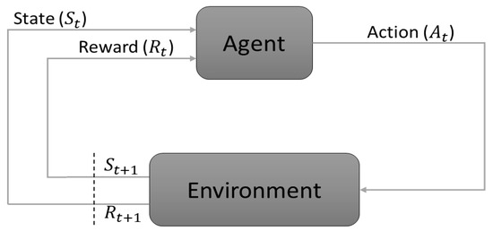
Figure 5. Reinforcement learning (Q-learning) process.

• The agent observes the current state, denoted as $S_t$ from a set of possible states S, and chooses an action $A_t$ from a set of possible actions A.
• Upon receiving the chosen action, the environment transitions to a new state $S_{t+1}$, also from S and provides a scalar reward $R_{t+1}$ from a subset of real numbers R.
• In response, the agent receives this reward, finds itself in the new state $S_{t+1}$, and determines its next action $A_{t+1}$ from A.

This cycle perpetuates until the agent reaches the terminal state $S_t$ from S. The agent’s primary objective is to formulate an optimal control policy that maximizes its cumulative discounted rewards over time, referred to as the expected discounted return G_T as shown in Equation (8) [10], where γ is the discounting factor, 0 < γ < 1.

$$G_t\doteq R_{t+1}+\gamma R_{t+2}+{\gamma }^2{R}_{t+3}+. . .=\sum _{k=0}^{\mathrm{\infty }} {\gamma }^k{R}_{t+k+1}$$

(8)

The fundamentals of Markov Decision Processes (MDPs) are closely related to the reinforcement learning (RL) problem [11]. A crucial feature of an MDP is its ability to guarantee that, regardless of an agent’s past experiences in different states, the current state contains all the necessary information to make decisions. Generally speaking, RL algorithms fall into two main categories: policy-based and value-based [11]. Within the value-based paradigm of reinforcement learning, a unique value function is utilized to determine the value or importance of every state. Under policy π, the state-value function is expressed as follows in Equation (9) when evaluating from a certain state:

$$v_{\pi }\left(s\right)\doteq {\mathbb{E}}_{\pi }\left[G_t\mid S_t=s\right]={\mathbb{E}}_{\pi }\left[\sum _{k=0}^{\mathrm{\infty }} {\gamma }^k{R}_{t+k+1}\mid S_t=s\right]$$

(9)

where ${\mathbb{E}}_{\pi }$ denotes the expectation under policy π. Similarly, under policy π, the action-value function, denoted as $q_{\pi }$, which represents the value of taking action a in state s, can be described in Equation (10) [10]:

$$\begin{array}{c}{q}_{\pi }\left(s,a\right)\doteq {\mathbb{E}}_{\pi }\left[G_t\mid S_t=s,A_t=a\right]={\mathbb{E}}_{\pi }\left[{\displaystyle \sum _{k=0}^{\mathrm{\infty }}} {\gamma }^k{R}_{t+k+1}\mid S_t=s,A_t=a\right]\\ \end{array}$$

(10)

Of all the action-value functions, the one that stands paramount is the optimal action-value function, articulated as Equation (11):

$${\mathrm{q}}_{\mathrm{*}}(\mathrm{s},\mathrm{a})\doteq \underset{\mathsf{\pi }}{\mathrm{m}\mathrm{a}\mathrm{x}} {\mathrm{q}}_{\mathsf{\pi }}(\mathrm{s},\mathrm{a}),$$

(11)

The Q-learning algorithm is an off-policy, value-based learning methodology within reinforcement learning (RL). Within this framework, the action-value function, denoted as Q, aims to emulate the optimal action-value function, q^* by bypassing the adherence to the present policy. Its update mechanism is articulated as in Equation (12) [12,27,28,29,30]:

$$\mathrm{Q}\left({\mathrm{S}}_{\mathrm{t}},{\mathrm{A}}_{\mathrm{t}}\right)\leftarrow \mathrm{Q}\left({\mathrm{S}}_{\mathrm{t}},{\mathrm{A}}_{\mathrm{t}}\right)+\mathsf{\alpha }\left[{\mathrm{R}}_{\mathrm{t}+1}+\mathsf{\gamma }\underset{\mathrm{a}}{\mathrm{m}\mathrm{a}\mathrm{x}} \mathrm{Q}\left({\mathrm{S}}_{\mathrm{t}+1},\mathrm{a}\right)-\mathrm{Q}\left({\mathrm{S}}_{\mathrm{t}},{\mathrm{A}}_{\mathrm{t}}\right)\right]$$

(12)

where α denotes the learning rate.

3.5. Design Adaptive PID Controller Using Q-Learning

To create an adaptive PID controller that learns using Q-learning, the fundamental ideas of the traditional PID controller must be seamlessly integrated with the reinforcement learning paradigms that are inherent in Q-learning. The following is a structured framework for conceiving such an integrated system (see Figure 6):

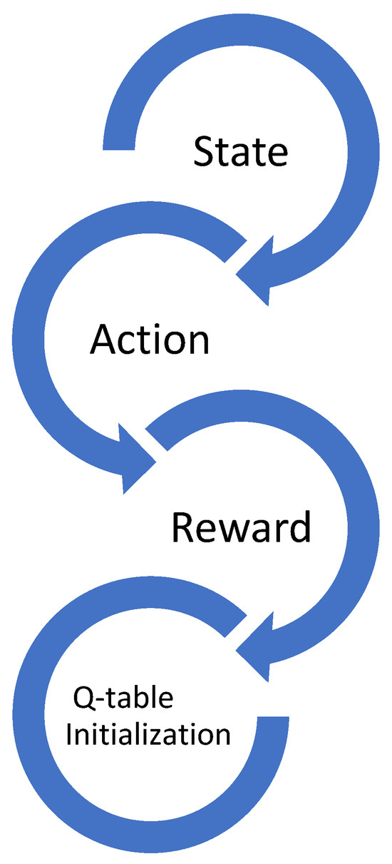
Figure 6. The structured framework for conceiving an integrated system.

• State: This indicates the current position of the system. In control challenges, the state usually contains the instantaneous error, denoted as e(t), and its temporal derivative, denoted as (de(t))/dt.
• Action: This refers to changes made to the PID parameters. In real-world scenarios, actions could include increasing, decreasing, or maintaining the current PID gains.
• Reward: Known as scalar feedback, the reward offers an assessment of the agent’s effectiveness. Here, possible metrics could be anything from the opposite of the absolute error to more complex assessment instruments that capture the system’s operational intelligence.
• Q-table initialization: Start with a tabular framework in which states characterize rows and the actions that correspond define the columns. The internal values of this matrix, known as Q-values, are then gradually improved based on the iterative feedback from the overall system.

The steps of an algorithm can be illustrated as follows:

• Action selection: using an exploration approach like ε-greedy, choose an action (change PID parameters) at each time step based on the current state.
• Take action: apply the PID controller to the system and adjust the PID settings.
• Observe reward: Calculate the reward and assess how the system responded. A PID controller’s objective could be to arrive at a predetermined point with the least amount of oscillation and settling time. Either the negative absolute error or a more complex function, such as the integral of time-weighted absolute error (ITAE), can be used to calculate the reward.
• Update Q-values: adjust the state-action pair’s Q-value by applying the Q-learning update rule.
• Loop: repeat this process for a specified number of episodes or until the Q-values converge.

The Q-values will direct the PID controller’s actions once the Q-table has been sufficiently trained. The course of action with the highest Q-value is the best one in a particular state. Since Q-learning has historically operated on discrete sets of states and actions, both the states and the actions must be discretized. For more complicated situations, neural networks (deep Q-learning) are one continuous version and approximator that can be used. To make sure the system is stable and adaptive, it should be tested in a variety of circumstances after it has been taught. A framework for combining Q-learning with PID controllers was explained in this overview.

4. Experimental Setup

The system model used in this study is depicted in Figure 7. It consists of two interconnected areas: Area 1 (generation) and Area 2 (loading). In Area 1, the generation units include Generator G1 with a capacity of 700 MW, and Generator G2, also with a capacity of 700 MW. In Area 2, the generation units include Generator G3 with a capacity of 719 MW, and Generator G4 with a capacity of 700 MW. The total generation capacity of the system is 2819 MW.

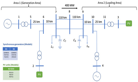
Figure 7. Kundur system model in PSSE.

The network is structured with several buses and transmission lines connecting the generators and loads. In Area 1, Bus 1 is connected to Generator G1 and Bus 2 to Generator G2. In Area 2, Buses 3 and 4 are connected to Generators G3 and G4, respectively. The two areas are interconnected through a series of transmission lines with specific distances between buses: 25 km between Bus 1 and Bus 5, 10 km between Bus 5 and Bus 6, 110 km between Bus 6 and Bus 7, another 110 km between Bus 7 and Bus 8, and a further 110 km between Bus 8 and Bus 9. From Bus 9 to Bus 10, the distance is 10 km, followed by 25 km from Bus 10 to Bus 11.

In addition, the network includes reactive power elements at specific buses to manage voltage levels and stability. Capacitor C7 with a capacity of 200 MVAr and Load L7 with a capacity of 967 MW are present at Bus 7, while Capacitor C9 with a capacity of 350 MVAr, and Load L9 with a capacity of 1767 MW are at Bus 9. The total active power of the investigated system is 2734 M. There is a power flow of 400 MW from Area 1 to Area 2, indicating the amount of transfer of power through the interconnection.

This model represents a typical high-voltage transmission network, which is used to analyze the power flow, stability, and reliability of the interconnected power system. The configuration ensures a robust system that can manage significant loads and maintain stable operations across the interconnected areas.

Kundur’s model is shown in Figure 7. In Kundur’s paradigm, power normally moves from Area 1 to Area 2, with two machines (G and PV) where G2 and G3 are replaced by PV in each area. The PSSE program was used to run simulations in order to assess the efficacy of the methods presented in this study. The PSSE model used in the simulations was obtained from the University of Illinois at Urbana-Champaign’s Illinois Center for a Smarter Electric Grid (ICSEG) [PSSE Models]. In order to assess the effectiveness of adopting PID control and examine the simulation findings, a comparison was carried out with a focus on four particular buses. These buses (Bus 1, Bus 3, Bus 7, and Bus 9) were selected based on an observability analysis which means two buses in the generation area and two buses in the loading area are required to observe the dynamic response of the system stability. In each area, two buses selected should observe the generation bus (Bus 1 and Bus 3) and the other two buses should be selected to observe the load buses (Bus 7 and Bus 9).

5. Results and Sensitivity Analysis

This section presents and highlights the results of studying the impact of renewable energy penetration on system stability, as well as the performance validation of the PID-RL control.

5.1. Impact of Renewable Energy Penetration on System Stability

The impact of high renewable energy penetration on system stability has been presented. Three scenarios have been studied and compared as follows: no photovoltaic (PV), 25% photovoltaic (PV)—700 MW, and 50% photovoltaic (PV)—1400 MW. The purpose of the study is to examine the performance of utilizing renewable energy penetration on the system stability of stations. The comparison of frequency difference responses for the three scenarios is shown in Figure 8. It refers to an electrical power system’s capability to keep a steady frequency in the face of fluctuations in the ratio of generation to demand. Variations in renewable energy production can result in demand as well as supply imbalances that negatively influence system frequency. Therefore, it is crucial to investigate the frequency response in order to guarantee system stability in these scenarios with a significant penetration of renewable energy. Three scenarios—none, 25%, and 50% photovoltaic (PV)—have been evaluated in the study that is being presented during a disturbance of generation reduction of 50 MW. As seen in Figure 8, the findings suggest that, in contrast to the scenarios with 25% and 50% PV penetration, the frequency response is more stable in the absence of renewable energy. On the other hand, tie-line active power, which represents the active power flow between interconnected systems, has high active power oscillation with 25% and 50% PV penetration. Conversely, when it comes to the flow of active power between interconnected systems, the study compared three scenarios: no photovoltaic (PV), 25% photovoltaic (PV), and 50% photovoltaic (PV). The findings revealed that the third scenario, with 50% PV penetration, exhibited lower stability in tie-line active power compared to the scenarios with no PV and 25% PV. This suggests that higher levels of PV penetration can contribute to improved stability in the flow of active power between interconnected systems as shown in Figure 9.

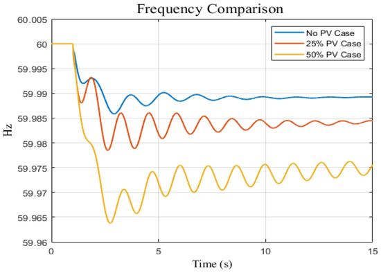
Figure 8. Kundur system model in PSSE frequency responses for three penetration scenarios: no PV, 25% of PV, and 50% of PV.

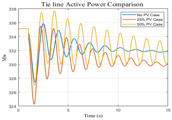
Figure 9. Tie-line active power response comparison for three penetration scenarios: no PV, 25% of PV, and 50% of PV.

Intriguing findings were obtained from the frequency differential response between the loading area and the generation area. Three different scenarios were investigated in the study: none, 25%, and 50% photovoltaic (PV). The results showed that in comparison to the scenario with no PV, the third scenario, with 50% PV penetration, showed less stability in frequency response between the loading area and the generation area. Additionally, it was observed that the 50% PV scenario exhibited lower stability than the 25% PV scenario. These results suggest that higher levels of PV penetration cannot contribute to enhanced stability in maintaining frequency balance between the generations and loading areas without adding controllers as shown in Figure 10.

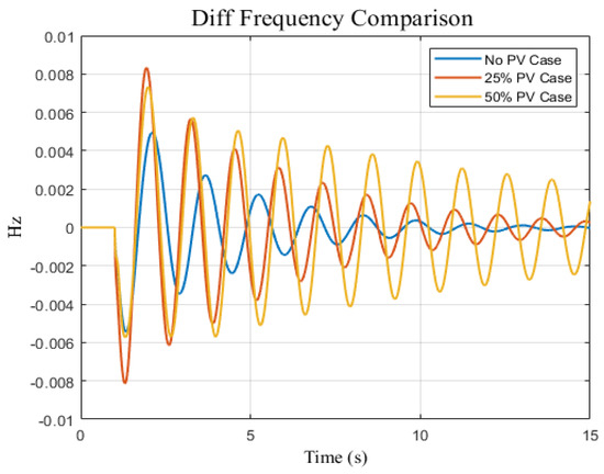
Figure 10. Frequency difference response between generation area and loading area for three penetration scenarios: no PV, 25% of PV, and 50% of PV.

5.2. PID-RL Control Performance Validation and Testing

Furthermore, the study conducted a performance validation of the PID-RL (Proportional-Integral-Derivative reinforcement learning) control technique, which combines traditional control theory with reinforcement learning algorithms. The validation process involved analyzing the performance of PID controllers and a base case scenario where no control input was applied to each EV station placement bus. This comparison allowed for an assessment of the effectiveness by utilizing a PID controller with a Particle Swarm Optimization (PSO) model for EV stations [19] and comparing it with a PID controller using RL and with no control input. By evaluating these different control approaches, the study aimed to determine their respective performances and identify the most suitable control strategy for regulating and stabilizing the power system in varying conditions.

The study conducted a comparative analysis of the stability of the electric vehicle (EV) system with 1% capacity (30 MW) under three control scenarios: no control input, PID-PSO [19], and PID-RL (reinforcement learning). The highest PV penetration level was selected (50%) and a disturbance of 50 MW generation reduction occurred in the first second. The results, as depicted in Figure 11, Figure 12 and Figure 13, highlighted that adding the EV system with PID-RL exhibited superior performance in terms of frequency response, tie-line active power response, and frequency difference response between the generation area and loading area, respectively. These findings indicated that the PID controller with RL optimization significantly enhanced the damping of the dominant oscillation mode within the EV system, resulting in improved stability when compared to both the EV system with PID-PSO and the EV system without any control input.

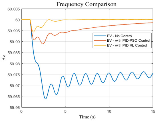
Figure 11. Frequency responses for three penetration scenarios for EV system with no control, PID-PSO control [19], and PID-RL control.

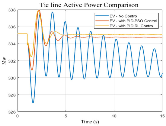
Figure 12. Tie-line active power response for three penetration scenarios for EV system with no control, PID-PSO control [19], and PID control.

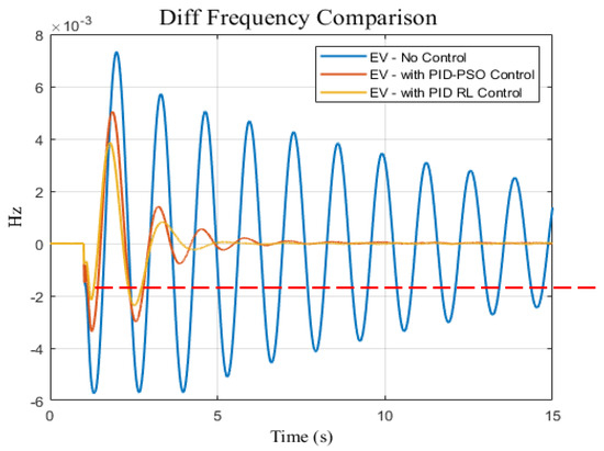
Figure 13. Frequency difference responses between generation area and loading area for three penetration scenarios for EV system with no control, PID-PSO control [19], and PID-RL control.

In order to study the sensitivity analysis of the results, two scenarios have been investigated. The first one is when the different magnitudes of generation reduction are considered—50 MW and 100 MW—whereas the PID-RL is used with an EV fast charging station of 1%. Figure 14 shows that the scenario of 100 MW generation reduction exceeds ±0.2 Hz operational limits for a primary response (10 s) while the statutory limit is ±0.5 Hz [31]. However, the integration of PID-RL enhances the frequency response for the same reduction and meets the operational frequency limits (Figure 14). The second sensitivity analysis scenario is applied to investigate different sizes of EV charging stations (0.75%, 1%, and 2%) regarding 21 MW, 30 MW, and 60 MW, respectively. The large size of the EV charging station as dynamic load positively enhances the frequency response can be seen in Figure 15 for the same PV penetration level and the same generation reduction disturbance.

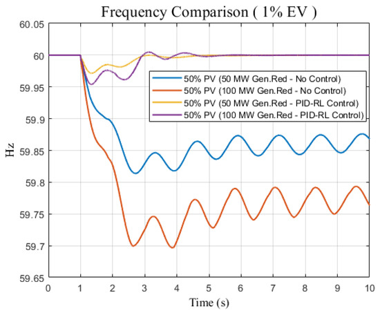
Figure 14. Frequency difference responses for different generation reduction disturbances for 50% PV and 1% EV systems with no control and PID-RL control.

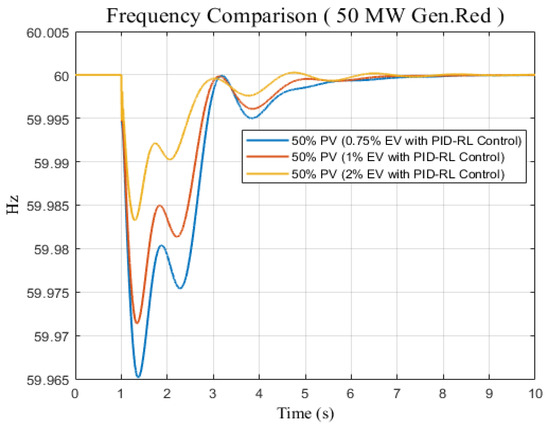
Figure 15. Frequency difference responses for different sizes of EV charging stations (0.75%, 1%, 2%) and a 50 MW generation reduction disturbance for 50% PV and PID-RL control.

6. Discussion

As discussed in the literature [17,18,19,20,21,22,23,24], using EVs to enhance system stability requires a fast response without any delay. As shown in Figure 11, Figure 12 and Figure 13, the system restored its stability within 4 s after the disturbance of 50 MW generation reduction occurred when PID-RL was used. The allowable time to restore the system stability is within 60 s after a disturbance has occurred. Moreover, the highest power flow between the interconnected areas occurred when PID-RL was used, whereas the active power oscillation was the lowest when PID-RL was used.

Comparing our proposed PID-RL controller technique with the PID-PSO proposed in [19], Figure 11 shows that our proposed technique has a faster frequency response compared to PID-PSO. Therefore, when an EV fast charging station is modeled as a dynamic load for frequency control, the PID-RL is the best controller option in terms of a fast frequency response.

According to [32], a comparison was conducted between the Genetic Algorithm (GA)—PID, Grey Wolf Optimizer (GWO)—PID, PSO-PID, and JAYA-PID in terms of the following: Peak Undershoot frequency (∆Hz), Settling Time (s) for both Area 1 and Area 2 as well as Peak Undershoot for power deviation in tie-line (MW) and Settling Time (s). To validate the fast response of our proposed PID-RL, a similar comparison to [32] is prepared in Table 1.

Table 1. A comparison of the dynamic response of the PID-RL and various controllers of optimized PID parameters with different approaches [32].

Methods	Performance Indices
	Area 1		Area 2		Tie-Line Power Deviation
	Peak Undershoot (∆Hz)	Settling Time (s)	Peak Undershoot (∆Hz)	Settling Time (s)	Peak Undershoot (∆MW)	Settling Time (s)
GA-PID [32]	0.059	44	0.105	52	55	45
PSO-PID [19]	0.031	24	0.013	21.5	9	19.5
GWO-PID [32]	0.024	21	0.011	18	7	17
JAYA-PID [32]	0.02	18	0.0085	15	4	11
PID-RL	0.005	4	0.004	4	3	5

The comparison shows how fast the PID-RL controller is compared to others thanks to the training stage of the controller using Q-learning. All optimized parameters of PID controller techniques—in the literature—have taken certain optimum values based on the stability problem; however, the power of reinforcement learning is that PID parameters are dynamic and change their values based on the best rewards of Q-learning as explained in Section 3. This fast response makes the proposed PID-RL suitable for a dynamic EV fast charging for load control with high performance, and it overcomes the problem of the delay discussed in the literature [17,18,19,20,21,22,23,24].

7. Conclusions

In summary, this research looked at two crucial areas: how the use of renewable energy affects system stability and how well the PID-RL control method performs. Three scenarios were assessed regarding the effects of the penetration of renewable energy: 25% PV, 50% PV, and no PV. The results showed that a higher degree of PV penetration (50%) contributed to the ability to improve the stability in tie-line active power flow between interconnected systems, even while the absence of renewable energy produced a more stable frequency response. This implies that higher PV penetration can improve stability in preserving active power flow and frequency balance. The study investigated three control scenarios: no control input, PID-PSO [19], and proposed PID-RL before moving on to the PID-RL control performance validation. The outcomes showed that in terms of frequency response, tie-line active power response, and frequency difference response, the EV system with PID-RL performed better than the other scenarios. In comparison to the EV system with PID-PSO and the EV system without control input, the PID controller with RL optimization greatly increased the damping of the dominant oscillation mode, resulting in increased stability. Overall, this study confirms the efficacy of the PID-RL control technique in stabilizing the EV system and offers insightful information about how the penetration of renewable energy affects system stability. These results can aid in the formulation of plans for incorporating renewable energy sources and improving control mechanisms in order to guarantee a more reliable and sustainable electrical grid. This research can be extended to different renewable energy resources such as wind turbines, and different electrical grids and models.

References

- Kroposki, B.; Johnson, B.; Zhang, Y.; Gevorgian, V.; Denholm, P.; Hodge, B.M.; Hannegan, B. Achieving a 100% renewable grid: Operating electric power systems with extremely high levels of variable renewable energy. IEEE Power Energy Mag. 2017, 15, 61–73. [Google Scholar] [CrossRef]
- Liu, H.; Zhu, L.; Pan, Z.; Guo, J.; Chai, J.; Yu, W.; Liu, Y. Comparison of mimo system identification methods for electromechanical oscillation damping estimation. In Proceedings of the 2016 IEEE Power and Energy Society General Meeting (PESGM), Boston, MA, USA, 17–21 July 2016; pp. 1–5. [Google Scholar]
- Ljung, L. System identification toolbox. In The Matlab User’s Guide; MathWorks Incorporated: Natick, MA, USA, 2011. [Google Scholar]
- Nan, J.; Yao, W.; Wen, J.; Peng, Y.; Fang, J.; Ai, X.; Wen, J. Wide-area power oscillation damper for DFIG-based wind farm with communication delay and packet dropout compensation. Int. J. Electr. Power Energy Syst. 2021, 124, 106306. [Google Scholar] [CrossRef]
- Ogata, K.; Yang, Y. Modern Control Engineering; Prentice Hall: Indianapolis, IN, USA, 2002; Volume 5. [Google Scholar]
- Kumar, M.; Panda, K.P.; Naayagi, R.T.; Thakur, R.; Panda, G. Comprehensive Review of Electric Vehicle Technology and Its Impacts: Detailed Investigation of Charging Infrastructure, Power Management, and Control Techniques. Appl. Sci. 2023, 13, 8919. [Google Scholar] [CrossRef]
- Xu, Z.; Cheng, C.; Li, Y. Static source error correction model based on MATLAB and simulink. In Proceedings of the IEEE 2019 Prognostics and System Health Management Conference (PHM-Qingdao), Qingdao, China, 25–27 October 2019; pp. 1–5. [Google Scholar]
- Eriksson, R.; Söder, L. Wide-area measurement system-based subspace identification for obtaining linear models to centrally coordinate controllable devices. IEEE Trans. Power Deliv. 2011, 26, 988–997. [Google Scholar] [CrossRef]
- Kumawat, A.K.; Kumawat, R.; Rawat, M.; Rout, R. Real time position control of electrohydraulic system using PID controller. Mater. Today Proc. 2021, 47, 2966–2969. [Google Scholar] [CrossRef]
- Pongfai, J.; Su, X.; Zhang, H.; Assawinchaichote, W. PID controller autotuning design by a deterministic Q-SLP algorithm. IEEE Access 2020, 8, 50010–50021. [Google Scholar] [CrossRef]
- Naeem, M.; Rizvi, S.T.H.; Coronato, A. A gentle introduction to reinforcement learning and its application in different fields. IEEE Access 2020, 8, 209320–209344. [Google Scholar] [CrossRef]
- Yao, Y.; Ma, N.; Wang, C.; Wu, Z.; Xu, C.; Zhang, J. Research and implementation of variable-domain fuzzy PID intelligent control method based on Q-Learning for self-driving in complex scenarios. Math. Biosci. Eng. 2023, 20, 6016–6029. [Google Scholar] [CrossRef] [PubMed]
- Ghosh, A. Possibilities and challenges for the inclusion of the electric vehicle (EV) to reduce the carbon footprint in the transport sector: A review. Energies 2020, 13, 2602. [Google Scholar] [CrossRef]
- Khalid, J.; Ramli, M.A.; Khan, M.S.; Hidayat, T. Efficient load frequency control of renewable integrated power system: A twin delayed DDPG-based deep reinforcement learning approach. IEEE Access 2022, 10, 51561–51574. [Google Scholar] [CrossRef]
- Dong, C.; Sun, J.; Wu, F.; Jia, H. Probability-based energy reinforced management of electric vehicle aggregation in the electrical grid frequency regulation. IEEE Access 2020, 8, 110598–110610. [Google Scholar] [CrossRef]
- Xu, P.; Zhang, J.; Gao, T.; Chen, S.; Wang, X.; Jiang, H.; Gao, W. Real-time fast charging station recommendation for electric vehicles in coupled power-transportation networks: A graph reinforcement learning method. Int. J. Electr. Power Energy Syst. 2022, 141, 108030. [Google Scholar] [CrossRef]
- Hussain, A.; Bui, V.H.; Kim, H.M. Deep reinforcement learning-based operation of fast charging stations coupled with energy storage system. Electr. Power Syst. Res. 2022, 210, 108087. [Google Scholar] [CrossRef]
- Amir, M.; Zaheeruddin Haque, A.; Kurukuru, V.B.; Bakhsh, F.I.; Ahmad, A. Agent based online learning approach for power flow control of electric vehicle fast charging station integrated with smart microgrid. IET Renew. Power Gener. 2022; Early View. [Google Scholar]
- Albert, J.R.; Selvan, P.; Sivakumar, P.; Rajalakshmi, R. An advanced electrical vehicle charging station using adaptive hybrid particle swarm optimization intended for renewable energy system for simultaneous distributions. J. Intell. Fuzzy Syst. 2022, 43, 4395–4407. [Google Scholar] [CrossRef]
- Wu, Y.; Wang, Z.; Huangfu, Y.; Ravey, A.; Chrenko, D.; Gao, F. Hierarchical operation of electric vehicle charging station in smart grid integration applications—An overview. Int. J. Electr. Power Energy Syst. 2022, 139, 108005. [Google Scholar] [CrossRef]
- Boopathi, D.; Jagatheesan, K.; Anand, B.; Samanta, S.; Dey, N. Frequency regulation of interlinked microgrid system using mayfly algorithm-based PID controller. Sustainability 2023, 15, 8829. [Google Scholar] [CrossRef]
- Wang, Y.; Chai, B.; Lu, W.; Zheng, X. A review of deep reinforcement learning applications in power system parameter estimation. In Proceedings of the IEEE 2021 International Conference on Power System Technology (POWERCON), Haikou, China, 8–9 December 2021; pp. 2015–2021. [Google Scholar]
- Liang, X.; Chai, H.; Ravishankar, J. Analytical methods of voltage stability in renewable dominated power systems: A review. Electricity 2022, 3, 75–107. [Google Scholar] [CrossRef]
- Teigenes, M. Provision of Primary Frequency Control from Electric Vehicles in the Nordic Power System. Master’s Thesis, NTNU, Trondheim, Norway, 2023. [Google Scholar]
- Xie, J.; Sun, W. A transfer and deep learning-based method for online frequency stability assessment and control. IEEE Access 2021, 9, 75712–75721. [Google Scholar] [CrossRef]
- Meridji, T.; Restrepo, J. Machine Learning-Based Platform for the Identification of Critical Generators-Context of High Renewable Integration. Available online: https://papers.ssrn.com/sol3/papers.cfm?abstract_id=4728247 (accessed on 24 April 2024).
- Cao, J.; Zhang, M.; Li, Y. A review of data-driven short-term voltage stability assessment of power systems: Concept, principle, and challenges. Math. Probl. Eng. 2021, 2021, 1–12. [Google Scholar] [CrossRef]
- Tejeswini, M.V.; Raglend, I.J. Modelling and sizing techniques to mitigate the impacts of wind fluctuations on power networks: A review. Int. J. Ambient Energy 2022, 43, 3600–3616. [Google Scholar] [CrossRef]
- Nguyen-Hoang, N.D.; Shin, W.; Lee, C.; Chung, I.Y.; Kim, D.; Hwang, Y.H.; Youn, J.; Maeng, J.; Yoon, M.; Hur, K.; et al. Operation Method of Energy Storage System Replacing Governor for Frequency Regulation of Synchronous Generator without Reserve. Energies 2022, 15, 798. [Google Scholar] [CrossRef]
- Schneider, K.P.; Sun, X.; Tuffner, F.K. Adaptive Load Shedding as Part of Primary Frequency Response To Support Networked Microgrid Operations. IEEE Trans. Power Syst. 2023, 39, 287–298. [Google Scholar] [CrossRef]
- Nedd, M.; Browell, J.; Bell, K.; Booth, C. Containing a Credible Loss to Within Frequency Stability Limits in a Low-Inertia GB Power System. IEEE Trans. Ind. Appl. 2020, 56, 1031–1039. [Google Scholar] [CrossRef]
- Annamraju, A.; Nandiraju, S. Coordinated control of conventional power sources and PHEVs using jaya algorithm optimized PID controller for frequency control of a renewable penetrated power system. Prot. Control Mod. Power Syst. 2019, 4, 1–13. [Google Scholar] [CrossRef]
Disclaimer/Publisher’s Note: The statements, opinions and data contained in all publications are solely those of the individual author(s) and contributor(s) and not of MDPI and/or the editor(s). MDPI and/or the editor(s) disclaim responsibility for any injury to people or property resulting from any ideas, methods, instructions or products referred to in the content. |
© 2024 by the authors. Licensee MDPI, Basel, Switzerland. This article is an open access article distributed under the terms and conditions of the Creative Commons Attribution (CC BY) license (https://creativecommons.org/licenses/by/4.0/).