Clean Energy Action Index Efficiency: An Analysis in Global Uncertainty Contexts

Abstract

Climate change, the scarcity of fossil fuels, advances in clean energy, and volatility of crude oil prices have led to the recognition of clean energy as a viable alternative to dirty energy. This paper investigates the multifractal scaling behavior and efficiency of green finance markets, as well as traditional markets such as gold, crude oil, and natural gas between 1 January 2018, and 9 March 2023. To test the serial dependency (autocorrelation) and the efficient market hypothesis, in its weak form, we employed the Lo and Mackinlay test and the DFA method. The empirical findings showed that returns data series exhibit signs of (in)efficiency. Additionally, there is a negative autocorrelation among the crude oil market, the Clean Energy Fuels Index, the Global Clean Energy Index, the gold market, and the natural gas market. Arbitration strategies can be used to obtain abnormal returns, but caution should be exercised as prices may increase above their actual market value and reduce the profitability of trading. This work contributes to the body of knowledge on sustainable finance by teaching investors how to use predictive strategies on the future values of their investments.

1. Introduction

Across the world, ecologically responsible investments are growing in popularity as more individuals worry about the future of the earth and seek methods to invest in businesses that support sustainable practices. The clean energy sector, which focuses on renewable energy sources including solar, wind, hydropower, geothermal, and biomass, is one of the most well-liked and rapidly expanding investment sectors [1].

Although there are still significant amounts of oil, gas, and coal under the soil, their extraction becomes more challenging and expensive. Countries that extensively rely on fossil fuels for their electricity production are more susceptible because of supply interruptions and price volatility [2].

Elie et al. [3] also argue that the risks connected with greenhouse gas emissions and the necessity to decrease reliance on fossil fuels are what are driving the rising demand for clean energy.

Investment prospects in the clean energy sector are developing quickly as governments all over the world raise their renewable energy and greenhouse gas emission objectives. Solar and wind energy have seen notable advances in clean energy technologies at the same time. These technologies are a feasible substitute for fossil fuels because they are becoming more affordable and effective. The economic advantages of clean energy, particularly in terms of job creation and local economic growth, are also being increasingly recognized [4,5,6].

Climate change, the limited availability of fossil fuels, improvements in clean energy technology, and the erratic nature of oil prices are just a few of the causes that have led to the widespread acceptance of clean energy as a viable substitute for dirty energy (such as crude oil). As part of the 2015 Paris Climate Accord, several nations made the commitment to transition to climate-resilient economies. Because of the increased interest among investors and policymakers as a result of the 2015 Paris Climate Accord, development in renewable energy initiatives have prospered [7,8].

As a result of the COVID-19 pandemic and the ongoing conflict between Russia and Ukraine, the price of energy has recently been severely impacted globally, causing several behavioral changes. The energy sector experienced a period of stagnation following the initial COVID-19 pandemic as several health and safety precautions were implemented to stop the virus’s spread. According to various studies, this led to a significant drop in energy consumption [9,10,11].

The decline in energy demand resulted in lower prices and forced a reduction in production levels [12]. Tensions between Saudi Arabia and Russia, the two largest oil producers, increased during this time. Saudi Arabia advised oil-producing nations to cut back on production as prices continued to drop to stabilize the market. Russia disagreed, which led to conflict between the two nations and had a negative effect on the economy of the sector. Energy supply fell behind demand as post-pandemic economic activity picked back up in 2021, which has resulted in increased prices and market volatility overall. The relationship between economic activity and energy use is unequivocally demonstrated [13].

At the start of the Russia–Ukraine conflict in 2022, the pandemic-related energy problem became worse. As a result of the conflict, Russia cut off the energy supply to European countries. Because of the numerous effects that threat and geopolitical events have on the volatility of energy prices, this factor not only contributed to the energy crisis in the European region but also to the instability of the global energy market [14].

Although there is a substantial body of academic research on price efficiency in the stock, bond, credit, exchange rate, commodity, and cryptocurrency markets [15,16], there is still a lot of room for further development of studies into the clean energy stock markets.

Understanding the efficiency of clean energy stock markets has important implications for various energy topics. First, it is argued that clean energy stock markets can affect energy consumption and many economic sectors. Second, given the strong link between market efficiency and the validity of price information, clean energy stock markets can influence dirty energy markets, such as crude oil. Given the importance of this theme, in this paper, we study the multifractal scaling behavior and efficiency of green finance markets, as well as traditional markets such as gold, crude oil, and natural gas between 1 January 2018, and 9 March 2023, which covers periods of low volatility and financial instability (2020 and 2022 events).

Based on the literature consulted, we expect to find signs of (in)efficiency in the time series under study.

The structure of the article is described as follows. In Part 2, a review of pertinent studies on the efficiency of clean energy stock markets is presented. In Section 3, the methods and data used to address research issues are described. In Section 4, the data analysis and conclusion interpretations are provided. Section 5 makes recommendations based on the information provided.

2. Literature Review

One of the distinguishing characteristics of an efficient market is how quickly new information is incorporated into stock prices. In such a market, new information is rapidly and completely reflected in pricing, and there is no potential to gain an edge by leveraging already-public information. Because of this, the market is always adjusting to new information, and stock values fluctuate as a result [17,18].

The EMH (efficiency market hypothesis) also makes the premise that market players are rational and act in their own best interests, in addition to presuming that information available on the market is free of charge. This implies that you will not let emotions or other illogical circumstances affect your judgment; instead, you will base your choices on all the information at your disposal. Recent research, however, has refuted this notion by demonstrating that psychological aspects, such as emotions, may have a big impact on financial decisions [19].

The EMH is nevertheless a widely recognized theory in finance, and many investors utilize it as the foundation for their investing strategies despite these obstacles. Yet, it is vital to keep in mind that no theory is foolproof, and that a variety of variables, such as political developments, economic conditions, and societal trends, can have an impact on financial markets.

As a result, it is crucial to approach investing cautiously and to weigh all the facts before making any decisions [20,21].

The Particularity of Clean Energy Stocks

This study will examine the two categories of clean energy financial markets: price indices (through an analysis of the Clean Energy Fuels Index and the S&P Global Clean Energy Index) and exchange-traded funds (ETFs) (by including the iShares Global Clean Energy ETF and the iShares Global Energy (SWX) ETF in the sample).

The Clean Energy Fuels Index reflects the price of the shares of Clean Energy Fuels Corp., a renewable energy company listed on the NASDAQ stock exchange. The company is focused on the acquisition and distribution of renewable natural gas (RNG) and conventional natural gas in the form of compressed natural gas and liquefied natural gas to the transportation markets of the United States and Canada. The S&P Global Clean Energy Index was formed with a target of 100 components to evaluate the performance of businesses involved in global clean energy in developed and emerging economies.

An ETF is a mutual fund investment that may invest in hundreds or even thousands of individual bonds, but it is traded as a share on a stock exchange throughout the day. Investments in renewable energy ETFs are made in companies that develop, produce, and use renewable energy technologies, such as wind, solar, hydropower, geothermal, biomass, biodiesel, and ethanol. Since they are made up of several assets, ETFs benefit from a reduced concentration of risk and are an excellent method to diversify any portfolio and be less susceptible to market volatility. However, since they are financial products, they are not immune to capital loss.

The financial incentives given to businesses for environmental performance in the energy industry have been the subject of certain studies. The financial and environmental performances of businesses in the energy industry were examined by Arslan-Ayaydin et al. [22]. The authors looked at the years 2000 to 2011 and found that companies in the energy sector with strong environmental performances outperform those in the same industry that do not incorporate green practices into their corporate strategies in terms of financial performance. Through the VIX index, they demonstrated that, particularly during times of low market volatility, investors may increase their profits by structuring their portfolios with renewable energy companies with strong environmental performances.

Wan et al. [23] studied the 2019–2020 period marked by the COVID-19 pandemic and showed that the adverse effects were more pronounced for fossil fuel industries than for renewable energy companies. The authors also note that these businesses have seen higher returns because investors have paid more attention to green energy companies over time. The growing adoption of green policies by various world economies is the primary cause of the sector’s enhanced appeal.

Portfolio managers’ interest in clean energy stocks has recently risen because of the additional advantages of investing in these companies. It is noteworthy that several recent studies indicate that investing in clean energy stocks may carry less risk than investing in the U.S. aggregated stock market index. For example, Uddin et al. [24] investigated the relationship between clean energy stock returns (ER) and aggregate share returns, changes in crude oil and gold prices, and exchange rates. Using a cross-quantilogram approach, the study concludes that the relationship between ER stock returns and changes in oil prices and the aggregate share index is not symmetrical between quants and is more significant with a higher number of lags. Furthermore, the study shows that the positive influence of exchange rates and gold returns on ER stock returns is only observed during extreme market conditions.

According to additional research, renewable energy stock indices can act as a hedge and safe haven for the crude oil and gold markets [3]. The same authors contend that government subsidies that stabilize the cash flows of green businesses make clean energy assets attractive investment opportunities. Clean energy reserves have characteristics of both the general stock market and energy products, and include companies involved in clean energy and related products and services. There is less opportunity for speculative activity in the clean energy market now that professional investors are participants. The interactions of market players using various informational time frames and interpretations may have an impact on the value of clean energy stocks.

Shahzad et al. [25] investigated the market efficiency of clean energy stock indices in the U.S., Europe, and globally. They found that the three markets exhibit a multifractal asymmetry after analyzing the data using asymmetric MF-DFA (multifractal detrended fluctuation analysis), with the U.S. market exhibiting this asymmetry because of long-range and fat-tailed correlation. Moreover, they discover that, while the American market is less efficient during the rising trend, the European and international markets are more efficient. The American market has nonetheless become comparatively more efficient over time.

Yao et al. [26] complementary examined and focused on China’s clean energy stock indices and analyzed their multifractal scale behavior and market efficiency using A-MFDFA (asymmetric and multifractal detrended fluctuation analysis) and A-MFDCCA (asymmetric and multifractal detrended cross-correlation analysis). The results show that the clean energy stock market is far from efficient and presents considerable asymmetries in both upward and downward fluctuations. Furthermore, the cross-correlation between crude oil price trends and low-carbon indices has significant multifractal characteristics. To limit risks, the study advises investors to undertake a hedging operation and pay attention to the counterparty market’s long-term effects.

In addition, due to investor interest, clean energy firms performed adequately during the pandemic, whereas fossil fuel companies did not. According to the study, green recovery programs can have a favorable impact on financial markets and promote the implementation of green measures.

Moreover, Thai [8], utilizing quantile-on-quantile regression and Granger’s causality methods, examined the connections between green bonds and other traditional assets such as Bitcoin, the S&P 500, the Clean Energy Index, the GSCI Commodities Index, and CBOE volatility. The findings show that other assets strengthen green bonds, and this effect is stronger in larger quantiles. The study recommends that policymakers think about tightening the eligibility requirements for green bond programs or restricting the use of green bonds for refinancing to promote renewable energy and energy efficiency. The author advises market players to raise funds to match the whole amount of investment required.

Kanamura [4] used in his empirical research the S&P Global Clean Energy Index (GCE), WilderHill Clean Energy Index (ECO), S&P/TSX Renewable Energy and Clean Technology Index (TXCT), S&P 500, WTI crude oil prices, and Henry Hub (HH) natural gas prices to examine the correlation between them. The findings demonstrate that, while the S&P 500 and energy prices have a positive but declining correlation, clean energy indices have positive and increasing correlations with crude oil or natural gas prices. For TXCT, correlations with WTI are generally positive and decrease as WTI increases, but correlations with HH are mostly positive and increase as HH decreases. Considering the results of GCE and ECO, it could imply that TXCT is still evolving as a clean energy index and is not yet fully operational.

Gustafsson et al. [27], underline the necessity of knowing the connections between energy metals and the clean energy stock markets. The findings point to statistically significant non-linear correlations between the studied markets. Except for cobalt, all energy metals exhibit a strong positive correlation with clean energy stock indices, and these correlations persist throughout periods of extreme volatility. The results support past studies on the hedging properties of precious metals, showing that gold and silver act as hedges for select clean energy stock indices.

3. Material and Methods

The daily price indices were obtained from the Thomson Reuters/Eikon platform, namely the Clean Energy Fuels Index, the S&P Global Clean Energy Index, the iShares Global Clean Energy ETF, the iShares Global Energy (SWX) ETF, crude oil (Brent), gold (Dow Jones), and natural gas (Dow Jones).

The sample data span the period from 1 January 2018 through 9 March 2023, which includes times of low volatility and financial instability (2020 and 2022 events).

The investigation was divided into stages, with the first analyzing the statistical properties of the studied series and estimating parameters such as the mean, standard deviation, asymmetry coefficients, and kurtosis, as well as applying the Jarque and Bera [28] test to infer the data series’ normality. To determine the stationarity of the time series, conventional panel unit root tests were applied, namely the Levin, Lin and Chu [29] (LLC), Breitung [30], and Im, Pesaran and Shin [31] (IPS) and for validation the Dickey and Fuller [32], and Perron and Philips [33] tests, with Fisher’s transformation.

Considering that the period under consideration includes times of volatility in financial markets caused by events in 2020 and 2022, the Clemente et al. [34] test was employed to infer the existence of unit roots in the observable time series components while taking structural breakdowns into consideration.

In a second stage, to answer the research question, we first applied the Brock and De Lima [35] test to identify nonlinear serial dependency in the time series under examination. To infer autocorrelation between series returns, the ratio of variances was examined using the Lo and Mackinlay [36] methodology. The premise of this test is that, in a non-autocorrelated process, the variance of the increases rises linearly with the observation range, i.e., the variance of the differences must be q times that of the first difference. The model consists of determining if the variance ratio for different ranges evaluated over time is equal to one. To confirm the autocorrelation’s plausibility, the results of the variance ratio must be statistically distinct from 1.

The ratio of variance is given by:

$$V{R}_q=\frac{{\sigma }_c^2\left(q\right)}{{\sigma }_a^2\left(q\right)}, where:$$

$${\sigma }_c^2\left(q\right)=\frac{1}{m} {\displaystyle \sum }_{t=q}^{nq}{\left(S_t-S_{t-q}-q\widehat{\mu }\right)}^2$$

$$m=q\left(nq-q+1\right)(1-\frac{q}{nq})$$

and

$${\sigma }_a^2\left(q\right)=\frac{1}{nq-1} {\sum }_{t=1}^{nq}{\left(S_t-S_{t-1}-\widehat{\mu }\right)}^2, \mathrm{in} \mathrm{which}:$$

$$\widehat{\mu }=\frac{1}{nq}\left(S_{nq}-S_0\right)$$

When $VR\left(q\right)=1$, the series follows a random walk process; however, when $VR\left(q\right)>1$, the series reveals the presence of positive correlations, and when $VR\left(q\right)<1$, the series exhibits negative correlations.

The detrended fluctuation analysis (DFA) approach, which allows for the investigation of temporal dependency in non-stable data series [21], was used to validate the reliability of the results produced.

Consider a set of data $x_k$, with $k=1,\dots , t$ equidistant observations. The first step of the DFA is the construction of a new series:

$$x\left(t\right)={{\displaystyle \sum }}_{k=1}^t{x}_k$$

The second step consists in obtaining the trend $z\left(t\right)$ of each fraction, through the method of the ordinary least squares, obtaining the series subtracted from the trend (detrended):

$$x_s\left(t\right)=x\left(t\right)-z\left(t\right)$$

The original application assumes that the trend present in each of the boxes is a linear trend, which is $Z\left(t\right)=at+b$, with subsequent applications indicating that it is likely to contain other polynomial trends [37].

For each box, the value of the trend equation is obtained by the method of the smallest squares and subsequently the root of the average square deviation between the series $x\left(t\right)$ and $Z\left(t\right)$, with the DFA function being given by the following equation:

$$F\left(s\right)=\sqrt{ \frac{1}{2N} {{\displaystyle \sum }}_{t=1}^{2N}{\left[x_s\left(t\right)\right]}^2}$$

Estimating the average of $F\left(s\right)$ for all the centralized boxes in s generates the value of the fluctuations $\langle F \left(s\right)\rangle$, in function of s. This estimate will be repeated for all values other than $s$, expecting a process of a power-law, i.e.:

$$\langle F \left(s\right)\rangle ~ s{\alpha }^{\alpha }$$

The DFA exponent represents the correlation properties of the time series, and means that if DFA = 0.5, there are no long-range correlations present in the series, and it remains in a state of equilibrium. If 0.5 < DFA < 1, the series is persistent, and the process is said to be long-term dependent with positive correlations. If 0 < DFA < 0.5, the series is antipersistent, and the process is said to be long-term dependent with negative correlations (see Table 1).

The calculated DFA coefficient can be interpreted as follows:

Table 1. Detrended fluctuation analysis (DFA).

Exponent	Type of Signal
${\mathsf{\alpha }}_{\mathrm{DFA}}<0.5$	long-range anti-persistent
${\mathsf{\alpha }}_{\mathrm{DFA}}$≃ 0.5	uncorrelated, white noise
${\mathsf{\alpha }}_{\mathrm{DFA}}$> 0.5	long-range persistent

Table 1. Detrended fluctuation analysis (DFA).

Exponent	Type of Signal
${\mathsf{\alpha }}_{\mathrm{DFA}}<0.5$	long-range anti-persistent
${\mathsf{\alpha }}_{\mathrm{DFA}}$≃ 0.5	uncorrelated, white noise
${\mathsf{\alpha }}_{\mathrm{DFA}}$> 0.5	long-range persistent

4. Results

4.1. Descriptive Statistics

Figure 1 shows the price movements of the seven financial markets over the course of the sample period. During the first wave of the COVID-19 pandemic, there was inevitably a decline in global demand for energy sources due to the implementation of limitations by world governments to prevent the virus’s spread, including the confinement of the population and the blocking of productive and commercial activity (oil, natural gas, and clean energies). Crude oil has seen a dramatic reduction in price as supply has greatly exceeded demand on a massive scale (see Figure 2).

The COVID-19 pandemic had a significant influence on the financial markets under study, causing drops in the first and second quarters of 2020, except for the gold market, which saw a price increase. This trend may have been driven by an increase in the demand for safe-haven assets, which was driven by the climate of uncertainty created by COVID-19 (see Figure 2).

During 2022, with the start of the war in Ukraine and, as a result, a reduction in the natural gas supply, the price of natural gas increased rapidly. Because of the looming scarcity of energy resources, the world’s economies have begun to increase their investments in clean energy.

Prior to presenting and analyzing the empirical findings on the serial dependency and efficiency of the financial markets under examination, we give a summary of the descriptive daily return data, as well as the stationarity results, of the following price indices: Clean Energy Fuels I, S&P Global Clean Energy Index, iShares Global Clean Energy ETF, iShares Global Energy (SWX) ETF, crude oil (Brent), gold (Dow Jones), and natural gas (Dow Jones).

Table 2. Descriptive statistics of the financial markets under study during the period from 1 March 2018 to 9 March 2023.

	Brent Crude Oil	Clean Energy Fuels	Global Clean Energy	Gold	Ishares	Ishrs	Natural Gas
Mean	0.000155	0.000598	0.001771	0.000245	0.000553	0.000544	−8.96 × 10−5
Std. Dev.	0.026217	0.049719	0.091985	0.009404	0.019220	0.018850	0.036237
Skewness	−1.234521	0.597367	−1.288416	−0.237269	−0.518329	−0.440643	−0.325035
Kurtosis	20.91207	14.58143	31.59122	8.009203	10.33827	9.116044	6.109057
Probability Jarque–Bera	0.000000 ***	0.000000 ***	0.000000 ***	0.000000 ***	0.000000 ***	0.000000 ***	0.000000 ***
Observations	1354	1354	1354	1354	1354	1354	1354

*** represent the rejection of the null hypothesis at a significance level of 1%.

summarizes the descriptive data of the price indices examined, revealing that all except natural gas had positive average daily returns.

As shown in Figure 3, the Global Clean Energy Index had the greatest average daily return (0.001771) during the research period; nevertheless, natural gas had a negative average daily return (−0.0000896).

Figure 4 shows the risk indicator (standard deviation) for the markets under investigation, revealing that the Global Clean Energy Index has the highest standard deviation (0.091985), and the gold market has the lowest (0.009404).

The data series are leptokurtic and asymmetrical, as indicated by the kurtosis values and asymmetry coefficients provided in Figure 5 and Figure 6, suggesting that they do not follow the requisites of a normal distribution. The conclusion of the Jarque and Bera test, which leads to the rejection of the null hypothesis (at a level of significance of 1%), supports this evidence.

4.2. Diagnostic

4.2.1. Time Series Stationarity

Testing the null hypothesis that the process generating the time series has an autoregressive unit root against the alternative that this process is a stationary trend is important in the empirical study of time series. In particular, the BDS test depends on the inference of the time series’ stationarity. To infer the presence of unit roots in the time series under study we used the panel tests of Levin, Lin and Chu [29] (LLC), Breitung [30], and Im, Pesaran and Shin [31] (IPS), and for validation Dickey and Fuller [32], and Phillips and Perron [33] tests.

The LLC and Breitung tests assume as the null hypothesis that all panels have a unit root. In contrast to these tests, the IPS test postulates that only a portion of the series is stationary. If the test statistic is more negative than the critical value, we can reject the null hypothesis and conclude that the time series is stationary. The Breitung test’s statistical value is −92.8583, the LLC test’s statistical value is 173.944, and the IPS test’s statistical value is −115.814, all of which result in H0 being rejected at a level of significance of 1%. As a result, we determine that the series is stationary.

The ADF test looks for a unit root to determine whether a trend exists in the data. The ADF test is comparable to the Phillips–Perron test, although the latter is a little more sophisticated. It looks for signs of predicted change in the data points. The time series is stationary if the data points change in a predictable manner. If the test statistic exceeds the critical value, the null hypothesis cannot be accepted, and the time series cannot be said to be stationary. The ADF and PP t statistic value of 1843.74 exceeds the critical value at a 1% level of significance, refuting the hypothesis that the data series exhibits a trend and supporting earlier findings that the series is stationary at initial differences.

The results of the unit root test are shown in

Table 3. Panel unit root tests applied to the financial markets under study during the period from 1 March 2018 to 9 March 2023.

Group Unit Root Test: Summary
			Cross-
Method	Statistic	Prob.**	sections	Obs
Null: Unit root (assumes common unit root process)
Levin, Lin & Chu t	−173.944	0.0000	7	9470
Breitung t-stat	−92.8583	0.0000	7	9463
Null: Unit root (assumes individual unit root process)
Im, Pesaran and Shin W-stat	−115.814	0.0000	7	9470
ADF—Fisher Chi-square	1843.74	0.0000	7	9470
PP—Fisher Chi-square	1843.74	0.0000	7	9471

** Probabilities for Fisher tests are computed using an asymptotic Chi-square distribution. All other tests assume asymptotic normality.

.

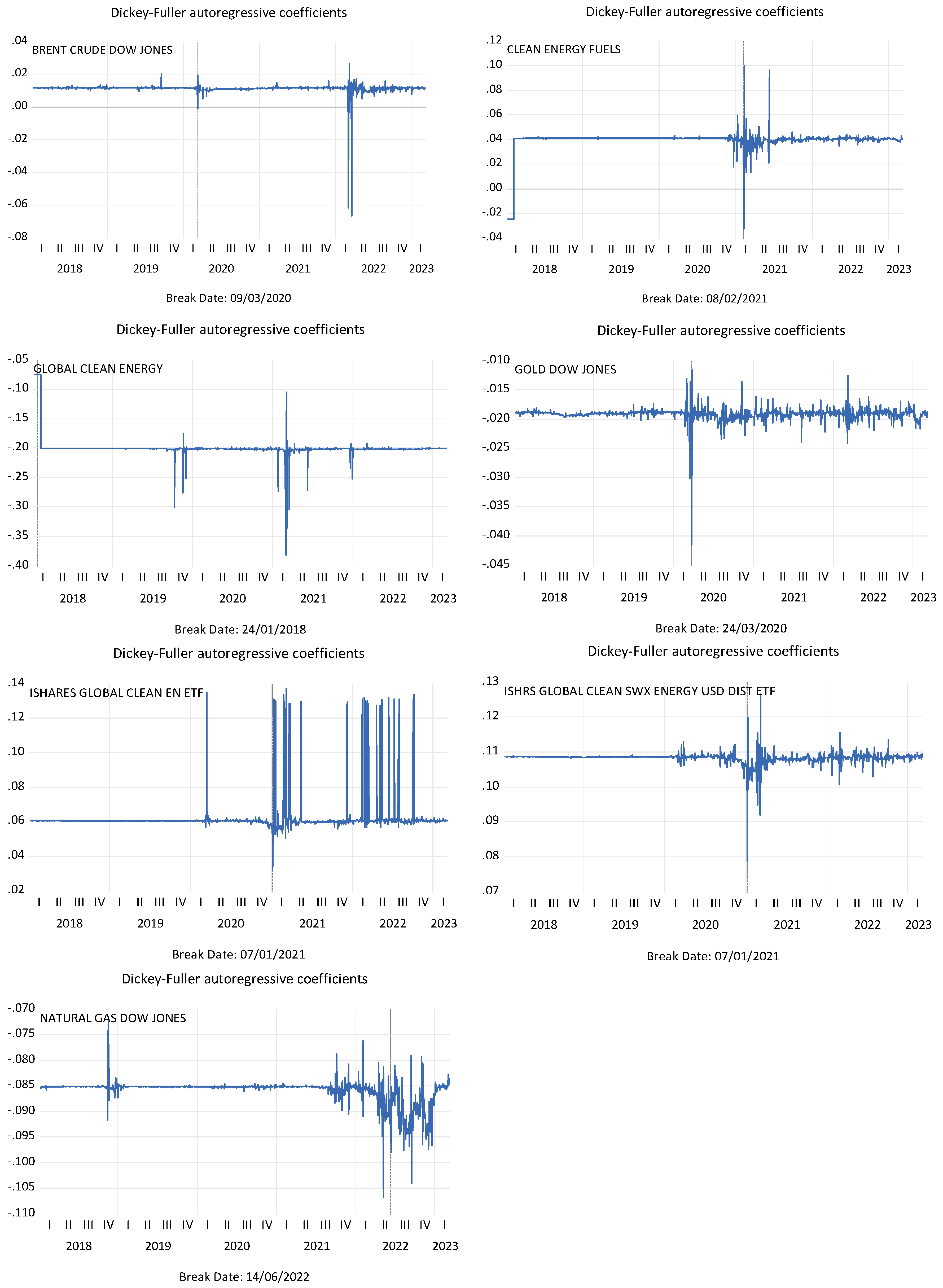
The study by Clemente et al. [34] was also necessary since it enabled the confirmation of unit roots while taking into account the potential for structural breakdowns in the time series and identifying the moment of their occurrence. This is due to the fact that the financial markets are now unstable and frequently subject to shocks brought on by the events of 2020 and 2022. All markets exhibit transitional imbalances, as illustrated in Figure 7, with the markets for dirty energy (crude oil and natural gas) and gold being particularly vulnerable to the shocks of the events of 2020 and 2022. In 2021, the clean energy markets exhibited volatility. The volatility of clean energy markets in 2021 may be attributed to leveraged investments in the industry.

4.2.2. Serial Dependence

To test the serial dependence, the Brock and De Lima [35] test was applied. The test’s null hypothesis assumes that the residual serial is independently and identically distributed. (i.i.d.). With the exception of the gold market in its second dimension, where the null hypothesis is only rejected at a degree of significance of 5%, the findings imply rejection of the null hypothesis at a level of significance of 1% for all time series in all dimensions (see

Table 4. Results of the BDS test applied to the financial markets under study during the period from 1 March 2018, to 9 March 2023.

BDS Test for Crude Oil (BRENT)
Dimension	BDS Statistic	Std. Error	z-Statistic	Prob.
2	0.016876	0.002599	6.492842	0.0000
3	0.036247	0.004129	8.778088	0.0000
4	0.051300	0.004917	10.43424	0.0000
5	0.059954	0.005124	11.70030	0.0000
6	0.063392	0.004942	12.82805	0.0000
BDS Test for Clean Energy Fuels
Dimension	BDS Statistic	Std. Error	z-Statistic	Prob.
2	0.020259	0.002572	7.877258	0.0000
3	0.038072	0.004080	9.330183	0.0000
4	0.048559	0.004852	10.00868	0.0000
5	0.052180	0.005050	10.33347	0.0000
6	0.052027	0.004863	10.69846	0.0000
BDS Test for Global Clean Energy
Dimension	BDS Statistic	Std. Error	z-Statistic	Prob.
2	0.022778	0.002952	7.716667	0.0000
3	0.039843	0.004700	8.476748	0.0000
4	0.047173	0.005610	8.408223	0.0000
5	0.048214	0.005862	8.224290	0.0000
6	0.047695	0.005669	8.413907	0.0000
BDS Test for Gold Dow Jones
Dimension	BDS Statistic	Std. Error	z-Statistic	Prob.
2	0.005789	0.002664	2.173212	0.0298
3	0.016060	0.004242	3.786072	0.0002
4	0.023335	0.005062	4.609951	0.0000
5	0.026482	0.005288	5.008143	0.0000
6	0.026392	0.005111	5.163640	0.0000
DBS Test for Ishares Global Clean Eergy Etf
Dimension	BDS Statistic	Std. Error	z-Statistic	Prob.
2	0.018124	0.002587	7.005582	0.0000
3	0.040525	0.004105	9.872918	0.0000
4	0.056914	0.004881	11.66085	0.0000
5	0.070098	0.005080	13.79832	0.0000
6	0.076621	0.004893	15.66015	0.0000
BDS Test for Ishares Global Clean (Swx) Energy ETF
Dimension	BDS Statistic	Std. Error	z-Statistic	Prob.
2	0.023454	0.002629	8.920287	0.0000
3	0.046955	0.004177	11.24106	0.0000
4	0.063969	0.004973	12.86232	0.0000
5	0.078078	0.005183	15.06335	0.0000
6	0.084883	0.004999	16.98125	0.0000
BDS Test for NATURAL GAS (DOW JONES)
Dimension	BDS Statistic	Std. Error	z-Statistic	Prob.
2	0.023727	0.002609	9.093599	0.0000
3	0.046691	0.004145	11.26397	0.0000
4	0.066183	0.004935	13.41045	0.0000
5	0.082197	0.005143	15.98124	0.0000
6	0.092390	0.004960	18.62734	0.0000

). Because the serial residues are not i.i.d., it is possible that the price indices under study either have linear returns or have a significant nonlinear component.

4.3. Methodological Results

4.3.1. Lo and MacKinlay Methodology

To examine whether the returns from the data series under study are autocorrelated over time, we applied the methodology proposed by Lo and MacKinlay [36].

The data were computed for the 2 to 16 lags in each case. The findings demonstrate that all stock indices reject the random walk hypothesis (see Figure 8). We may deduce from the variance ratio values that the returns of the crude oil market, the Clean Energy Fuels Index, the Global Clean Energy Index, the gold market, and the natural gas market are negatively autocorrelated over time because they all display values below the unit. As the EFTs’ variance ratio values are higher than those of the unit, their returns are positively autocorrelated over time. Positive news and markets with positive serial autocorrelation might cause price gains as investors get more optimistic about these markets’ prospects. Markets that deliver negative serial autocorrelation and bad news, on the other hand, might cause a sell as investors grow increasingly pessimistic about the prospects of these markets in the future. Due to a decreased risk of being swayed by overly dramatic responses to news or information, investors may find it simpler to make more informed investing decisions.

4.3.2. Detrended Fluctuation Analysis (DFA)

The DFA exponents for the time series were calculated in order to verify the validity of the previously obtained results (see

Table 5. DFA results. The hypotheses are $H_0$: α = 0.5 and $H_1$: α ≠ 0.5.

Market	Expoent DFA (Tranquil)	Expoent DFA (Stress)
Crude oil (BRENT)	0.52 ≅ 0.0206 ($R^2$ = 0.97)	0.56 *** ≅ 0.0029 ($R^2$ = 0.97)
Clean Energy Fuels	0.61 *** ≅ 0.0010 ($R^2$ = 0.97)	0.54 ** ≅ 0.0014 ($R^2$ = 0.98)
Global Cean Energy	0.46 ** ≅ 0.0019 ($R^2$ = 0.98)	0.44 ** ≅ 0.0012 ($R^2$ = 0.98)
Gold DOWN JONES))	0.46 ≅ 0.0248 ($R^2$ = 0.97)	0.44 ** ≅ 0.0064 ($R^2$ = 0.98)
Ishares Global Clean Energy EFT	0.50 ≅ 0.0082 ($R^2$ = 0.98)	0.59 *** ≅ 0.0023 ($R^2$ = 0.99)
Ishares Global Energy (SWX) EFT	0.51 ≅ 0.0106 ($R^2$ = 0.98)	0.58 *** ≅ 0.0019 ($R^2$ = 0.99)
Natural gas (DOW JONES)	0.55 ** ≅ 0.0027 ($R^2$ = 0.97)	0.52 ≅ 0.0136 ($R^2$ = 0.98)

***, ** represent the level of significance of 1% and 5%, respectively.

). We split the sample into two subperiods to test the predictability of time series returns: tranquil subperiod from 1 January 2018 to 31 December 2019, and stress subperiod from 1 January 2020 to 9 March 2023. According to the estimated DFA exponents for the tranquil subperiod, the returns of the crude oil (0.52 ≅ 0.0206), the gold (0.46 ≅ 0.0248), the iShares Global Clean Energy ETF (0.50 ≅ 0.0082), and the iShares Global Energy (SWX) ETF (0.51 ≅ 0.0106) are all in equilibrium and are therefore priced randomly. Long memory (persistence) in returns may be seen in both the natural gas market (0.55) and the Clean Energy Fuels Index (0.61). Only the Global Clean Energy Index (0.46) exhibits antipersistence signs.

All markets, except for natural gas (0.52 ≌ 0.0136), rejected the random walk hypothesis during the stress subperiod. The returns of the Crude Oil Market (0.56 ≅ 0.0029), Clean Energy Fuels Index (0.54 ≅ 0.0014), iShares Global Clean Energy EFT (0.59 ≅ 0.0023), and iShares Global Energy (SWX) EFT (0.58 ≅ 0.0019) demonstrate long memory (persistence). On the other hand, the returns of the gold market (0.44 ≅ 0.0064) and the Global Clean Energy Index (0.44 ≅ 0.0012) show an antipersistent pattern.

5. Discussion

In this paper, we investigate the multifractal scaling behavior and efficiency of green finance markets, as well as traditional markets such as gold, crude oil, and natural gas between 1 January 2018 and 9 March 2023, which covers periods of low volatility and financial instability (2020 and 2022 events).

To determine whether series returns are autocorrelated over time, the Lo and MacKinlay methodology was applied. The results presented in Figure 8 allow us to conclude that, based on the values calculated for the Lo and MacKinlay test, under the premise of homoscedasticity, the random walk hypothesis was rejected for daily returns at the 5% significance level for the entire sample at all lag days.

The returns of the crude oil market, the Clean Energy Fuels Index, Global Clean Energy Index, the gold market, and the natural gas market are negatively autocorrelated, which implies that series returns present a reverse average. Reverse average trading implies that, despite significant fluctuations, the price of an asset returns to its average levels. This approach requires the investor to first determine the average value of a financial instrument, sell when the value exceeds the average, and buy when the value declines. On the other hand, positive autocorrelation signals may be detected in the returns of the EFTs, which implies that if the market is “up” today, it is more likely to stay that way tomorrow.

The estimation of the DFA exponents was utilized to support these conclusions and provide a response to the question of whether the markets under examination are efficient in their weak form. DFA is a method useful for analyzing time series that appear to be long-memory processes and white noise. Fractal analysis enables synergy between fundamental and statistical approaches to dynamic market forecasting.

The market’s response to the events of 2020 (the COVID-19 pandemic and Saudi Arabia and Russia’s price war) and 2022 (the Russian invasion of Ukraine) may be observed throughout the stress subperiod results. We can see that the crude oil market (0.52 ≌ 0.0206 → 0.56 ≌ 0.0029), the gold market (0.46 ≌ 0.0248 → 0.44 ≌ 0.0064), the iShares Global Clean Energy EFT (0.50 ≌ 0.0082 → 0.59 ≌ 0.0023), and the iShares Global Energy (SWX) EFT (0.51 ≌ 0.0106 → 0.58 ≌ 0.0019), all changed from an equilibrium state to rejecting the random walk hypothesis during the stress subperiod compared with the tranquil subperiod. Comparatively, the predictability of the crude oil market, the iShares Global Clean Energy EFT, and the iShares Global Energy (SWX) EFT showed a significant change, moving from an equilibrium state to exhibit long memories (persistence). The gold market, on the other hand, changed from being in a state of stability to displaying some antipersistence.

Meanwhile, the Clean Energy Fuels Index continued to demonstrate long memory (0.61 ≌ 0.0010 → 0.54 ≌ 0.0014) while the Global Clean Energy Index showed antipersistence (0.46 ≌ 0.0019 → 0.44 ≌ 0.0012).

The evidence presented by Shahzad et al. [25] and Yao et al. [26] that the clean energy indices they studied are far from efficient markets and have exhibited an asymmetrical behavior is supported by our findings.

These results challenge the notion of an efficient market, allowing investors to consider methods for forecasting future returns based on their prior observations. Long memory (persistence) in a time series means that a high value in a series will probably be followed by another high value, and this impact will probably last for a very long period in the future. When the time series shows some antipersistence, the returns have a greater likelihood of cycling between high and low values for an extended period.

According to our study, traders should try to anticipate whether stocks will rise or decrease in markets that display (anti)persistence in their returns since technical analysis helps us to identify a trend based on historical data and predict future stock movements. This will make it feasible to recommend viable business plans for taking advantage of changing trends. However, there may be risks involved with employing technical analysis that need to be considered because previous data do not guarantee that the same movement will occur again in the future.

The probability of cyclical dependency in the short/long term is lower for markets whose price formation follows a random walk process, which implies that it is not useful to place a lot of confidence in technical analysis because past values have no influence on the present. Therefore, we propose that, in this scenario, the approach will involve fundamental analysis, in which investors will have to determine the actual intrinsic value of a company utilizing the important information that has been made publicly available. Fundamental analysis is a method, but it has its limitations. When enough investors choose which stocks to buy based on the same signals and data, they might themselves trigger the anticipated movement. Our study contributes to the body of research that has already been done on the efficiency and dynamic linkages in the markets for clean and dirty energy during times of high market uncertainty. Our findings additionally have relevance for market regulators, policymakers, and individual and institutional investors. By providing evidence about the predictability of the series under analysis, the data offered assist investors who want to have some exposure to the clean energy markets in their portfolio to make more specialized, probably more profitable, and sustainable decisions. In addition to the practical implications that these results have for investors, they will provide the necessary information to regulators and political decision-makers so that they can provide transparency and access to information strategies that will help to address the market’s inefficiencies.

6. Conclusions

Despite rising public knowledge and interest in renewable energy, clean energy firms still have a tiny market valuation compared with the traditional energy industries. This is partially because the clean energy sector is still seen as a new and unproven area, which may give investors a sense of uncertainty and risk. Nonetheless, the clean energy sector is anticipated to expand quickly in the next years as more nations and people throughout the world realize how important it is to switch to greener energy sources. This expansion is anticipated to be fueled by a mix of financial government incentives, developments in clean energy technologies, and rising consumer demand for environmentally friendly and sustainable goods and services. Moreover, more environmental, social, and governance (ESG) expenditures are anticipated to accelerate the growth of the clean energy industries.

This paper examines the efficiency in the Clean Energy Fuels Index, the S&P Global Clean Energy Index, the iShares Global Clean Energy ETF, the iShares Global Energy (SWX) ETF, the crude oil market (Brent), the gold market (Dow Jones), and the natural gas market (Dow Jones). We conclude that understanding the efficiency of clean energy markets is important for several reasons. First, as the world turns toward renewable energy consumption, it is important to understand how the clean energy stock market is working. This knowledge can help investors make informed decisions about where to invest their money, which can have a significant impact on the development and growth of clean energy technologies. Second, understanding the efficiency of clean energy stock markets can help policymakers design more effective policies to promote the growth of clean energy industries. Finally, understanding the efficiency of clean energy markets can provide a broader insight into the functioning of markets and the factors that influence efficiency.