Review

A Review of Research on Advanced Control Methods for Underground Coal Gasification Processes

Institute of Control and Informatization of Production Processes, Faculty BERG, Technical University of Košice, Němcovej 3, 042 00 Kosice, Slovakia
*
Author to whom correspondence should be addressed.
Energies 2023, 16(8), 3458; https://doi.org/10.3390/en16083458
Submission received: 29 March 2023 / Revised: 10 April 2023 / Accepted: 12 April 2023 / Published: 14 April 2023

Abstract

:
Underground coal gasification (UCG) is a clean coal mining technology without significant environmental impacts. This technology can also be used in deep, hard-to-reach seams or deposits affected by tectonic disturbances, where conventional mining is impossible. Several techniques and methods have been investigated worldwide to support the process control of UCG. Global research focuses on the control of UCG operating parameters to stabilize or to optimize the performance of the underground reactor during energy conversion. This paper studies recent research in the field of UCG control and compares individual control techniques and possibilities for practical application. The paper focuses on advanced control methods that can be implemented in an in situ control system (e.g., adaptive control, extremum seeking control, and robust control). The study investigates control methods that ensure desired syngas calorific value or maximization. The review showed that robust control techniques such as sliding mode control and model predictive control have the most significant potential, and achieve the best results despite their complexity. In addition, some methods have been investigated through simulation or experimentally. The paper aims to give the reader an overview of the given issue and to alert the practice to recent research in the given area.

1. Introduction

Underground coal gasification (UCG) is a coal mining technology from deposits that are inaccessible for extraction via mining mechanisms. This technology is also suitable for coal deposits with tectonic faults [1]. UCG has the potential to be applied in coal mines at great depths, where the mining and geological conditions are unfavorable, and where the risk of explosion is high. In such mines, it is necessary to monitor the concentration of toxic and flammable gases constantly [2]. Aghalayam [3] performed a comprehensive overview of UCG field trials and practice. In addition, information about the successful operation of commercial UCG around the world can be found in various publications and technical reports (e.g., [4,5,6,7,8,9,10,11,12,13]).
Commercial gasification needs a skilled workforce, technology contributors, industry standards, and an adequate regulatory framework. The main issue for the commercial UCG operator is the stable production of high-quality syngas. The problem can be the gradual enlarging of the cavity, the enlarging of the reactor cross-section, the reduction in the gas velocity in the reactor, the decrease in the Reynolds number, the flow turbulence criteria, and the decrease in oxidizer efficiency [14]. Nevertheless, the results show that UCG can extract 52–68% of the chemical exergy of the coal [15]. The energy conversion efficiency for UCG is a crucial research topic because it directly affects gasification projects’ economic and environmental benefits [16].
UCG technology is implemented by drilling an injection and production well into an underground coal seam, igniting the coal, and promoting gasification chemical reactions using gasification agents [12,13,17,18,19]. UCG processes are supported by injecting gasification agents (i.e., air, oxygen, and steam) and extracting the produced syngas. UCG represents spatially and thermally distributed reaction zones, where the coal oxidation, reduction, and pyrolysis regions overlap [1,3,13,20,21,22,23,24].
The calorific value of the produced syngas is the most critical operational parameter of the UCG. However, maintaining the calorific value of syngas during gasification at the desired values can be a problem. Therefore, the control system should determine the optimal values of the manipulation variables to track the desired syngas calorific value or underground temperature and to ensure the course of the chemical reactions. The composition of the syngas depends on the coal type and the gasification agent injected. Gases such as H 2 , CO 2 , CO, and CH 4  represent the essential calorific components of the syngas [25]. For example, syngas with a low calorific value is produced when air and water vapor are used (e.g., Chinchilla, 3–5 MJ/m 3 ). On the other hand, oxygen and water vapor are injected for medium to high calorific values of syngas. Although gasification with oxygen is more expensive, it brings a higher stability to the produced syngas (e.g., Spanish trials yielded 13 MJ/m 3  of dry gas after gas clean up) [26,27].
The motivation for writing this review study was to inform the professional public about recent developments in advanced UCG control. The study focuses on advanced control methods that ensure a desired syngas calorific value or maximization. Unfortunately, only a few researchers deal with this issue. The direct control of UCG processes (i.e., a basic process control system) is provided by essential control elements, e.g., actuators, sensors, and programmable logic controllers (PLCs), in combination with a supervisory control and data acquisition system (SCADA) to ensure operation and the automation of production. In control theory, advanced process control represents a wide range of techniques and technologies implemented in control systems. The algorithms of UCG advanced control are developed as an alternative or a higher level to basic control, especially to improve syngas production performance or economic parameters. This class includes algorithms of advanced regulatory control (ARC) (e.g., adaptive feedback control), extremum seeking control (ESC), optimal control (OC), robust control, model-based control, multivariable model predictive control (MPC), and control based on artificial intelligence (e.g., machine learning control (MLC)). The benefit of the automatic control of UCG, built on advanced control algorithms, can be higher control accuracy, reduction in the human decision about control interventions, and the possibility of more accessible communication with higher levels of control.
The nature of process information and the possibility of identifying UCG processes for their modeling determines the options for the design of the control system. The underground geo-reactor develops during the UCG (e.g., the movement of the combustion front, groundwater, cavity enlargement, etc.), which complicates the modeling of individual processes [28]. However, the UCG process is evolving, and underground conditions may change continuously. For this reason, it is necessary to constantly monitor the underground environment and to adapt to the operational parameters of the UCG [7].
At the stabilization level of the control, in addition to calorific value and temperature, it is also necessary to maintain a low concentration of oxygen in the syngas. Control algorithms are usually tested through simulation and on laboratory ex situ reactors. For example, the control techniques on stabilization level for UCG based on discrete controllers were studied in [28]. Another example can be the simple computer feedback control with the process monitoring of the ex situ UCG reactor presented in [29]. Adaptive control can adapt the controller properties to changing operating conditions (e.g., a change in operating mode, most often in the form of a change in the pressure conditions).
Adaptive control techniques are used to adjust the control strategy in response to changes in the process environment. This type of control can improve the performance and stability of UCG processes, especially in the presence of unpredictable or time-varying conditions. Furthermore, this approach makes dealing with uncertainties in the process possible. Adaptive control can be built on linear or non-linear regulators. Furthermore, it can be controlled with a model, model-free control (e.g., extremum seeking control), or control based on machine learning [30]. The advanced control of UCG based on continuous extremum seeking was also experimentally tested, where control without a model [31,32] or with a model, Ref. [33] was applied.
Optimal control refers to mathematical optimization techniques to find the control inputs that minimize a given cost function, subject to a set of constraints that describes the system’s dynamics. The goal of optimal control is to find the “optimal” control input that achieves the desired control objective with minimum cost. These techniques typically involve mathematical optimization algorithms considering complex interactions between various process variables and the control inputs. The proposal for optimal coal gasification control based on Iterative Adaptive Dynamic Programming (ADP) and neural network can be found in [34,35].
On the other hand, robust control is concerned with designing controllers that can handle uncertainties and disturbances in the system being controlled. The goal of robust control is to ensure that the system remains stable and performs well, even in the presence of model uncertainties, measurement noise, and other types of disturbances. Among the most well-known robust control techniques applied in UCG to stabilize syngas calorific value is sliding mode control (SMC) [36,37,38] and multivariable  H  robust control [39,40]. The disadvantage of robust control is that it is necessary to spend more effort to build a mathematical model and to propose an appropriate unmeasured states estimator. While optimal control can lead to high-performance solutions, it may only sometimes be robust to uncertainties and disturbances. Robust control, on the other hand, may sacrifice some performance for the sake of robustness. Therefore, optimal and robust control are complementary techniques that can be combined to achieve high performance and robustness. Optimal control and robust control are two distinct control techniques with different goals and methods, although there is some overlap between them.
One of the main disadvantages of in situ UCG is the need for more process control and predictability. Predictive control or model predictive control (MPC) is a form of optimal control in which a dynamic model of the system being controlled is used to predict its behavior over a finite time horizon. Based on these predictions, an optimization problem is solved to find the control inputs that minimize a cost function subject to constraints on the system’s state and input variables. MPC is often used when there are constraints on the system, such as constraints on the allowable control inputs or the state of the system. Although MPC algorithms are programmed in many programming languages, it is necessary to properly design the internal prediction model and to program the state estimator to estimate the unknown states of the UCG. This type of advanced UCG control was recently investigated by researchers in [41,42].
Various models have been developed over the years to improve the knowledge of the UCG process and process control [3,12]. These models solve the calculation of transient temperature profiles, the determination of gas velocity and coal consumption, the prediction of cavity formation, the operating pressure, the flow rates of gasification agents, the ratio of injected oxidizers, and syngas composition and its production rate. Perkins [18,21,43,44] performed extensive research work focused on UCG modeling. Perkins proposed a UCG model to quantify the effects of changes in operating conditions and coal properties on the growth rate of a local cavity. The development of control-oriented mathematical models, which make predicting various process states and outputs possible, is a trend in UCG research [45]. In addition, mathematical models or the study of model predictions allow for a better assessment of the internal processes of the UCG. Understanding brings a better ability to design, control, and predict performance. For example, in [36,37,38], a control-oriented one-dimensional packed bed model of the UCG to estimate the syngas composition was proposed. This model was connected with the sliding mode controller to stabilize the syngas heating value. Magnani et al. [46] proposed a two-dimensional mathematical model that studies the effects of the process variables on the total heat recovery via the gasification process. The model simulates the UCG stream method using produced gas stoichiometry. Other packed bed models to predict the behaviors of the geo-reactor were developed in [29,47,48,49].
Some works (e.g., [33,50,51]) only investigated the prediction of output UCG parameters (e.g., syngas calorific value, and syngas composition or temperature in the oxidation zone) or proposed a thermodynamic model for the model-based optimization of gasification agents (e.g., [52,53,54,55]). Another approach for syngas composition prediction was based on partial differential equations [50]. The goal of control is achieved by measuring process variables with a programmed algorithm that ensures the calculation of control interventions. However, some UCG variables could be more problematic to measure directly (i.e., contact sensing). Therefore, indirect methods are used. For example, in the case of determining the underground temperature in a georeactor, soft-sensors are used based on the measurement of radon emanation, carbon isotopes in syngas, and the CO/CO + CO 2  ratio in syngas [56,57]. Temperature or temperature field predictions based on mathematical models are gaining popularity (e.g., [58,59]). The research has also focused on developing models for predicting underground temperature and the temperature field. Based on the energy and material balance equations, an axial model was built to calculate the temperature distribution in the coal seam along the gasification channel [60]. Kostúr [61] proposed a two-dimensional model of the temperature field of an underground reactor based on Fourier’s partial equation but expanded via heat exchange between the solid and liquid phases. Other researchers investigated the modeling of the behavior of the temperature field using a hybrid supercomputer [62]. The analysis of the results of mathematical modeling showed that the modeling of automatic control systems and forecasting systems, including robust control, can be significantly extended by using hybrid supercomputers.
In recent years, UCG models based on machine learning have come to the attention of researchers. Machine learning models can support the UCG process control, where they can be used as soft-sensors for temperature in the georeactor, for calorific value, or in syngas composition [63]. Applying neural networks to temperature prediction was investigated by Ji and Shi [64], and syngas composition prediction by Guo et al. [65]. Neural networks (NN), support vector algorithms (SVM), and multivariate adaptive regression splines (MARS) were well compared in [51]. Other proposals of the machine learning models of coal gasification were presented in [34,35].
In the following section, a more detailed overview of the main principles of advanced UCG control, which have been researched in recent years, will be provided. The principles and results of adaptive control at the stabilization level of UCG, extremum seeking control, robust control, and model-predictive control will be presented. These dilution techniques were tested through simulation on models, ex situ reactors, and others applied to in situ gasification. Individual approaches to advanced UCG control will be compared in the discussion, and their advantages and disadvantages will be pointed out.

2. Overview of UCG Advanced Control Techniques

2.1. Adaptive Feedback Control

In UCG, stabilizing and optimizing gasification agent flows is needed to stabilize underground temperature and syngas production. The increasing oxygenation of coal results in increased temperatures in the oxidation zone so that reduction can occur. This results in an increase in the calorific value of the syngas. An increase in operating pressure can positively affect methane and hydrogen production [66]. The ideal temperature in the oxidation zone is above 1000  C. The following three main principles of UCG management are used in practice (see Figure 1) [28]:
  • Over-pressure control—the flow of the injected oxidizer is adjusted to stabilize underground temperature, syngas composition, or its calorific value. Increasing the amount of gasification agent can increase the calorific value of the syngas. The disadvantage of this type of control is a possible gas leak to the surrounding strata or cooling of the reduction zone with too much gasification agent [28,67,68].
  • Under-pressure control (also called burning control)—the exhaust ventilator adjusts under pressure. Air enters the georeactor under negative pressure (i.e., through an injection well or various cracks) and supports the smoldering of the coal. There are no syngas leaks into the surrounding strata. At the same time, the ventilator sucks the syngas to the surface for further processing [28,69,70].
  • Combined control—those as mentioned above are used.
The geo-reactor changes over time, and there is a need to continually improve the control and to adapt the controller to changes in the system. Kačur et al. [28,71] proposed an adaptive control system for the stabilization of temperature and oxygen concentration in syngas based on a discrete PID controller (see Figure 2). The proposed control system can also be used to stabilize the syngas calorific value.
The gasification in the ex situ reactor was supported by air injection or was controlled under pressure at the outlet. The modified Ziegler-Nichols method adopted from [72] performed the initial controller setup. Figure 3 shows the temperature stabilization by the discrete controller that adjusts airflow. The controller parameters were adapted to between 1300–1400 min from the beginning. The maximal effect of CO 2  consumption is at temperatures of above 1000  C. These are the ideal theoretical conditions for reacting the entire amount of CO 2  to CO, assuming the presence of coal [28].
On the same principle, a regulation for reducing the oxygen in the produced syngas was also proposed. In this case, the regulated negative pressure from the ex situ reactor was used as the manipulated variable. The pressure was varied, utilizing the speed of the exhaust ventilator (i.e., the frequency of the asynchronous motor inverter was adjusted). Figure 4 shows the stabilization of oxygen concentration in syngas via controlled sucking pressure, which is adjusted by the exhaust fan motor power frequency (Hz).
In this case, the discrete controller was adapted based on the new identification of the controlled system at 4800 min.
Another example shows the reduction in oxygen concentration using a controlled airflow (see Figure 5). The tuned controller continually decreases airflow to ensure the desired oxygen concentration value in the syngas. This oxygen reduction should have an increased syngas calorific value during the experiment.
Figure 6 shows the course of continuously reduced oxygen concentration in syngas by the adaptive controller, and the corresponding syngas calorific value for a long time. From the point of view of the control goal, it is necessary to maintain the oxygen concentration at close to zero.

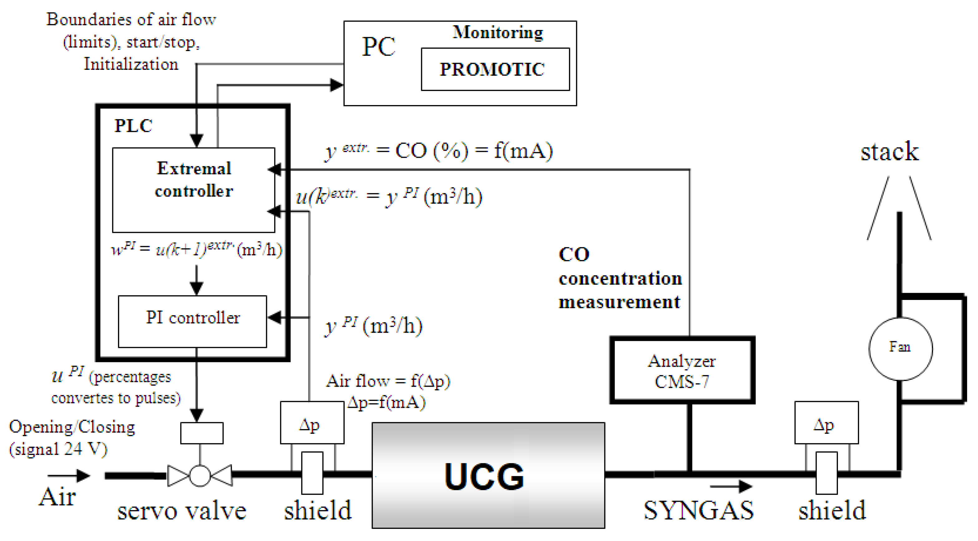
2.2. Extremum Seeking Control

Extremum seeking control (ESC) is a subclass of adaptive control aimed at optimizing the process in a steady state. This control technique has been successfully applied to control biochemical processes using the model [73] or without the model [74]. Another well-known approach to extremum seeking control is based on perturbations [75,76].

2.2.1. Model-Free ESC

Kostúr and Kačur [32] suggested an alternative method for controlling UCG using extremum seeking control. This technique, first introduced by Leblanc in the 1920s [77], is a clever way to drive a system towards the optimal value of a measured variable of interest [78,79].
In the proposed ESC algorithm, the concentration of CO in syngas was maximized as an indicator of syngas quality. The objective function was expressed as follows [67,68]:
y ( k ) = 1 n i = 1 n φ CO ( i )
where the optimized variable at step k is denoted by  y ( k )  (%). The measured CO concentration in the syngas is represented by  φ CO  (%). k is the index of the optimized period for the extremum seeking control ( τ 0 , o p t ), while i represents the index of the sampling period ( τ 0 , s t a b ) at the stabilization level. The variable n corresponds to the number of sampling periods ( τ 0 , s t a b ) that occur during  τ 0 , o p t .
CO concentration enters the ESC algorithm as the average concentration over time,  τ 0 , o p t . ESC is based on continuously optimizing the airflow as the leading gasification agent. If the UCG process is under steady-state conditions, the ESC algorithm seeks a new optimum as a new desired flow rate. The PI controller uses this desired value to stabilize the airflow. The optimized setpoint (i.e., desired airflow) is calculated as the following [67]:
w ( k + 1 ) = u ( k ) + sgn ( Δ w ( k + 1 ) ) · Δ V / m ,
where  u ( k )  represents the average value of the manipulation variable in the step k (m 3 /h), calculated as  u ( k ) = 1 n i = 1 n u i  t.j. as the average air flow elapses during  τ 0 , o p t . Furthermore, it is true that  Δ u ( k ) = u ( k ) u ( k 1 )  a  Δ y ( k ) = y ( k ) y ( k 1 ) . Parameter  w ( k + 1 )  is the desired variable of ESC in the step  k + 1  (i.e., the new desired airflow) that enters the PI controller as a new setpoint (m 3 /h) (see Figure 7). Parameter k is the time step, and  Δ V / m  is the increment of the desired value w. When initializing the algorithm, constant  Δ V  is empirically determined by the flow stabilization quality and  m = 1 .
If  sgn ( Δ w ( k + 1 ) )  changes from (+) to (–) or from (–) to (+), it is then needed to modify the parameter m (i.e.,  m = m + 1 ) and to continue the algorithm from the beginning. For the calculation of Equation (2), the Table 1 can be used.
Increasing the desired airflow at the start of ESC was gradually adapted, and CO concentration has been maximized in syngas (see Figure 8). The optimized air flow maximized the coal conversion to CO, an endothermic reaction at higher temperatures of above 800  C. The increased concentration of CO in the syngas was also reflected in the increased calorific value of the syngas.
The gases CO and CO 2  are products of the gasification process. Increasing the temperature increases the production of CO, and the effective activation energy decreases. Therefore, the CO/(CO + CO 2 ) ratio is also an important indicator during gasification. Considering the Boudouard reaction, carbon monoxide (CO) dominates in high temperatures (see Figure 9).
The ratio CO/(CO + CO 2 ) is increased with an increasing concentration of CO and decreases with an increased concentration of CO 2 . At a higher operating pressure, the production of CO is reduced.
Figure 10 shows the behavior of the highest measured temperature, and the calculated calorific value from the gas composition. The behavior that is shown is from the whole experiment. The figure shows that the lower calorific value (1–9 MJ/m 3 ) dominates at lower temperatures (700–1000  C). However, the higher calorific value (9–14 MJ/m 3 ) also occurs at a higher temperature (i.e., 1000–1400  C).
Figure 11 shows the behavior of the measured concentration and the ratio of CO/(CO + CO 2 ). The duration of the experiment is the same as in Figure 10. It can be said that the ratio value is higher at higher temperatures by comparing the two images. The figure shows that the lower value of the ratio (0 to 0.25) is dominant at lower temperatures (700–1000  C). At a higher temperature (i.e., 1000–1400  C), the value of the ratio is higher (i.e., 0.25–60).
An example of a decreased ratio and calorific value is at the time of 135 h from ignition. At this time, it significantly reduces the maximum temperature. Research has shown that the CO/(CO + CO 2 ) ratio decreases with the increasing pressure of the oxidizer, and increases with increasing temperature. When searching for an extreme of this ratio, the aim is to find the maximum. Theoretically, the maximum value of the ratio is equal to the number 1. The increased value of this ratio represents a higher concentration of CO, and ultimately, a higher calorific value.
An alternative task of the extremal controller can be to control the airflow to achieve and to maintain the maximum value of the CO/(CO + CO 2 ) ratio. Figure 12 shows the CO/(CO + CO 2 ) ratio maximization behavior during the experiment with gasification. The extremal controller was tested during an experiment with gasification on the laboratory gasifier. The extreme was reached after 70 min from the start of the controller. Then, the controller increased the ratio to 0.125, and 120 min was maintained.
Figure 13 shows the behavior of the calorific value and the maximized ratio. While maximizing the mentioned ratio, the calorific value was increased to 0.85 and 1.2 MJ/m 3 .
A model-free extremum seeking control based on perturbations was experimentally tested to optimize several manipulation variables [31]. A perturbation signal at the system input and observing its effect on the output can be used to estimate the objective function. In the case of the optimization of three UCG manipulation variables, the following vector was defined [80]:
u ¯ = u 1 u 2 u 3 T ,
where  u 1  refers to the desired airflow (m 3 /h) or the servo valve opening that can be adjusted using a PI controller or directly via digital pulses; similarly,  u 2  corresponds to the desired flow rate of oxygen injected to the oxidation mixture (m 3 /h). Finally, the third control variable  u 3  represents the regulated under-pressure on the outlet (Pa), equivalent to the frequency of the asynchronous motor power (Hz). Altering the motor power frequency causes changes in the ventilator’s speed, affecting the outlets under pressure (Pa).
Figure 14 shows the connection scheme of ESC with three manipulation variables. The ESC was applied to maximize syngas calorific value during experiments on an ex situ reactor.
The objective function, which expresses the maximum calorific value, can be defined as follows [31]:
J k ( u ¯ ) 1 n i = 1 n H j · Δ τ j M A X ,
where the objective function  J k ( u ¯ )  is calculated as the average value of the heating values from the buffer, denoted by  H j  (MJ/m 3 ), which represents the j-th heating value of the syngas recorded in the buffer with the size of n. Parameter k represents the index of the control period. The manipulation variables in vector  u ¯  are optimized with sampling period  τ 0 , o p t , and sampling on the stabilization level  Δ τ j  is given by step j.
Alternatively, the optimality criterion can also express the maximum concentration of the i-th syngas component (e.g., CO, CH 4 , or H 2 ), the maximum CO/(CO + CO 2 ) ratio in the syngas, the maximum gain of chemically bound energy, the maximum volume of the produced syngas, or the maximal temperature in the oxidation zone [25].
The optimization problem was solved using the Gradient method with constraints. The control law is as follows [81,82].
u ¯ i + 1 = u ¯ i + h · J ( u ¯ i ) = u ¯ i + h · J u 1 i , J u 2 i , J u 3 i T ,
where in each new control step i, a new set of optimized manipulation variables, denoted as  u ¯ i + 1 , is calculated based on the previous set of optimized variables, represented as  u ¯ i . The value of iterative constant h is chosen to ensure that the values in  u ¯ i + 1  will lead to the existence of the objective function and its continual maximization (i.e.,  J ( u ¯ i + 1 ) > J ( u ¯ i ) ). The gradient  J ( u ¯ i )  consists of partial differentials of the cost function concerning the variables in vector  u ¯ i . This vector can be calculated using loading perturbations on individual manipulation variables during UCG.
In each optimization step  τ 0 , o p t , the ESC algorithm calculates a new vector of gradients  J ( u ¯ i )  based on the introduced perturbations on individual manipulation variables. Subsequently, a new action intervention is calculated according to Equation (5) and the current value of the objective function (4), i.e.,  J k ( u ¯ i + 1 )  is determined, which is compared with the value of the objective function from the previous step  J k ( u ¯ i )  to evaluate convergence to the extreme. In addition, the algorithm considers the set limit values of the manipulation variables (3) and the limitation that applies to the concentration of oxygen in the syngas. All calculations (i.e., the calculation of gradients and objective functions, as well as new action interventions) are performed only in the steady state of the objective function (4). This state is determined by the standard deviation, which is compared with an experimentally determined threshold value. The principle of model-free extremum seeking control is shown in Figure 15.
Figure 16 shows the result of ESC with three manipulation variables during 10 h, where the increasing heating value of syngas from 4.4 to 8 MJ/m 3  can be observed. This behavior was obtained by decreasing airflow, increasing oxygen added to the mixture, and reducing the power of the exhaust ventilator [25,31,67,68,80].
Another example (see Figure 17) shows the result of ESC with two manipulation variables. Optimizing the injected air flow and outlet pressure from the ex situ reactor increased the calorific value from 2.17 to 7.4 MJ/m 3 .

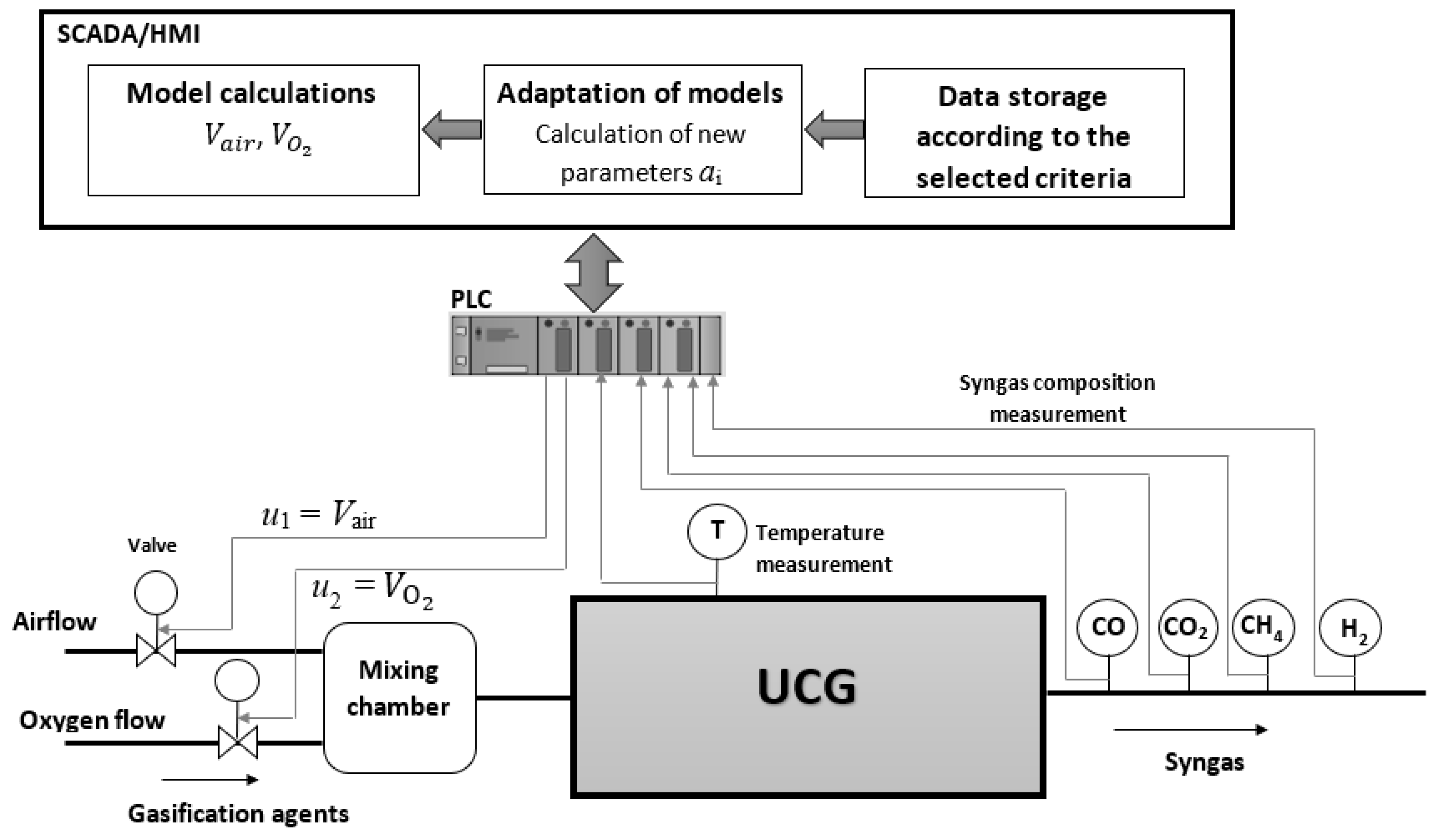
2.2.2. Model-Based ESC

An important goal in UCG is to maintain syngas production with the highest possible calorific value. Since syngas production occurs at higher temperatures, ensuring these temperatures in the georeactor is necessary. For this reason, we can divide the coal gasification process into two phases from the point of view of management:
  • Reaching high temperatures—circa 1000  C,
  • The production of syngas with the highest possible calorific value—i.e., an almost zero concentration of O 2  and the highest possible concentration of CO, CH 4 , and H 2  in the syngas.
A simple ESC algorithm based on a continuous adaptation of regression models was proposed in [25,33,83]. The algorithm consisted of two parts:
  • Recording measured data to the dataset according to the selected criteria or the stage of the gasification process,
  • Estimation of new model parameters for manipulation variables (i.e., adaptation).
The proposed control system continuously stores the measured data from the UCG with the selected sampling period  τ 0  into four separate datasets. Each dataset (i.e., buffer with shift) was created for a fixed number of n historical records.
Figure 18 shows the principle of the proposed control system. Each buffer recorded data for when a specific gasification quality criterion was reached. Then, the updated datasets were used to calculate the regression parameters of the models (i.e., the models of the manipulated variables). The criteria for the various type of control are as follows:
  • The calorific value of syngas ( H s y n g a s : 1 <  H s y n g a s  < 3 MJ/m 3 ,
  • The calorific value of syngas ( H s y n g a s ): 3 <  H s y n g a s  < 6 MJ/m 3 ,
  • The calorific value of syngas ( H s y n g a s ):  H s y n g a s  > 6 MJ/m 3 ,
  • The maximum temperature in the coal channel ( T m a x ):  T m a x  > 900  C.
The subroutine performs repeated calculations of the control model parameters according to the set adaptation period  τ 0 , c a l c .
Regression models were designed in three variants according to the proposed criteria. For example, the first model type could continuously calculate the optimal injected airflow and the oxygen flow based on five measured parameters. Therefore, the model equations for the first control type have the following form [25]:
u 1 V air ( k ) = a 0 + a 1 · V air ( k 1 ) + a 2 · φ CO ( k 1 ) + a 3 · φ CO 2 ( k 1 ) + a 4 · φ CH 4 ( k 1 ) + a 5 · T ( k 1 ) ,
u 2 V o 2 ( k ) = a 0 + a 1 · V O 2 ( k 1 ) + a 2 · φ CO ( k 1 ) + a 3 · φ CO 2 ( k 1 ) + a 4 · φ CH 4 ( k 1 ) + a 5 · T ( k 1 ) ,
where k represents the control step of the sampling period  τ 0 V a i r  and  V O 2  represent the flow rates of injected air and oxygen to the mixture (m 3 /h);  φ i  is the concentration of CO, CO 2 , and CH 4  in the syngas (%); and T represents the coal temperature in the gasification channel ( C).
The second type of model refers to the ratio of the flow rates of gasification agents and the highest temperature in the gasification channel  T m a x . The structure of this model is the following [25]:
u 1 V air ( k ) = a 0 + a 1 · V air ( k 1 ) V O 2 ( k 1 ) + a 2 · φ CO ( k 1 ) + a 3 · φ CO 2 ( k 1 ) + a 4 · φ CH 4 ( k 1 ) + a 5 · T max ( k 1 ) ,
u 2 V O 2 ( k ) = a 0 + a 1 · V air ( k 1 ) V O 2 ( k 1 ) + a 2 · φ CO ( k 1 ) + a 3 · φ CO 2 ( k 1 ) + a 4 · φ CH 4 ( k 1 ) + a 5 · T max ( k 1 ) .
The third model type aims to achieve the necessary temperature for syngas production. The models regarding the ratio of gasification agents and the maximum temperature  T m a x  in the channel are in the linear and quadratic form. The structure of the model is as the following [25]:
u 1 V air ( k ) = a 0 + a 1 · V air ( k 1 ) V O 2 ( k 1 ) + a 2 · T max ( k 1 ) + a 3 T max 2 ( k 1 ) ,
u 2 V O 2 ( k ) = a 0 + a 1 · V air ( k 1 ) V O 2 ( k 1 ) + a 2 · T max ( k 1 ) + a 3 T max 2 ( k 1 ) .
For a better illustration, Figure 19 and Figure 20 show the simulation (i.e., offline) verification of the first model. It is evident from Figure 19 and Figure 20 that the discrepancies between the actual and the modeled flow rates are minimal. The measured airflow and oxygen flow are represented in red and modeled in green. The online control using the first model type during the UCG experiment on the ex situ reactor is depicted in Figure 21, where the heating value of the syngas was achieved to be 10 MJ/m 3  by regulating the airflow.

2.3. Robust Control

Robust control has potential applications in UCG processes. For example, a feedback control system is robust if it maintains basic qualitative properties such as stability, quality of regulation, etc., under the influence of various disturbances, including changes in the parameters of the controlled system. In recent years, research on UCG control possibilities has been intensively directed to robust control techniques that have brought about significant progress in implementing advanced control. Model-based robust control uses a mathematical model of the UCG process being controlled to design a controller robust to uncertainties and variations in the system. In the following subsections, an overview of the investigated robust control techniques for UCG will be made.

2.3.1. Sliding Mode Control

For UCG systems with nonlinearities, in situ disturbances, and parametric uncertainties, a control technique is required which can keep a constant desired heating value of syngas, even though the design procedure is performed based on an approximate model [38]. Uppal et al. [36,37] proposed a one-dimensional (1-D) packed bed model of UCG that was used in closed-loop with robust sliding mode control (SMC) [84]. The proposed SMC could maintain a syngas calorific value at the desired value by manipulating the injected gas mixture in the presence of disturbances and model uncertainties [84].
The model could forecast various UCG parameters such as solid temperature, syngas composition, and the rates of different chemical reactions. However, most of these parameters are difficult to measure, although they make it possible to analyze the dynamics of UCG. Therefore, the stoichiometric coefficients for the coal pyrolysis reaction entering the model were optimized to compensate for the uncertainty in some coal properties. The optimization was performed using sequential quadratic programming (SQP) [37].
Sliding mode control is a nonlinear control technique that achieves robustness against uncertainties and disturbances by forcing the system trajectory to converge to a prescribed sliding surface in a finite time.
The basic idea behind sliding mode control is to design a control law that drives the system trajectory onto a sliding surface, a hyperplane in the state space. Once the system trajectory reaches the sliding surface, it is constrained to stay on it, which makes the system behavior insensitive to uncertainties and disturbances that affect the dynamics outside the sliding surface [85].
The sliding mode control law consists of the control signal and the sliding function. The control signal is designed to force the system trajectory to converge to the sliding surface. In contrast, the sliding function is a scalar function of the state variables that takes a constant value on the sliding surface, and changes sign when the system trajectory crosses the sliding surface. The sliding function is used to construct the control signal to drive the system trajectory onto the sliding surface and maintain it there.
The principle of sliding mode control can be summarized as follows: if a system can be transformed into a special form called the sliding mode, then it can be controlled robustly by designing a control law that forces the system to remain on the sliding surface [86].
Figure 22 shows a sliding mode control block diagram applied to syngas calorific value stabilization. The control signal in the SMC consists of two parts: the reaching mode and the sliding mode. The reaching mode brings the system’s state to a sliding surface (see Figure 23); switching control ( u s w ) is required [87]. Furthermore, in the sliding mode state, there is an equivalent control ( u e q ) to keep the state system stable.
The authors in [37] have used the time model of the UCG reactor and the following first-order controller:
U = u e q + u s w ,
where U is the vector of the control variables  u i  (i.e., control effort),  i = 1 , 2 , 3 u 1  is the molar flow rate (moles/cm 2 ·s) of H 2 O;  u 2  is the molar flow rate of O 2 , and  u 3  is the molar flow rate of N 2  of a mixture pumped into the injection well (i.e., the input to the plant).
The equivalent and switching control can be expressed as follows [37]:
u e q = L C T γ 1 γ 2 ,
u s w = K · sgn s , s = s x , t = e ,
where  K · sgn s  represents the so-called switching part (i.e., the discontinuous part) of the control that provides resistance to changes in parameters and external disturbances while also causing chattering.  u e q  is a continuous part of the controller output that takes system trajectories to the sliding manifold; s represents the sliding function. The positive constant  K > 0  determines the speed of the trajectory converging to the sliding surface, parameter x represents the state vector (i.e., if the state model presents), t is the time (s),  e = y y d  is the control error,  y d  is desired value of the calorific value (kJ/mol), y is the measured calorific value (kJ/mol), and L is the length of the UCG reactor or physical model (cm). Parameter  C T  represents the sum of the syngas component concentration and  γ 1 γ 2  depends on rates of chemical reactions. If  s > 0  then sgn s = + 1 , otherwise if  s < 0  then  sgn s = 1   [37].
The sliding mode control (SMC) principle involves bringing the system’s state to the sliding surface and the central point. The sliding surface represents a state where the switching function (s) is zero. The upper and lower bounds of the sliding surface are determined by a limiting switching value,  ± Δ . When the state  x ( t )  is greater than  Δ , the switching is turned off; conversely, if  x ( t ) < = Δ , the switching is turned on. The system transitions between stable and unstable trajectories to reach the sliding surface, ultimately leading to error convergence to zero.
In the subsequent research, Uppal et al. [88] optimized a 1-D packed bed model to compensate for the uncertainty in coal and char ultimate analysis, and in the steam-to-oxygen (O 2 ) ratio. The optimization problem was solved using sequential quadratic programming (SQP) to minimize the error between the simulated and the measured calorific values. The model was validated with a twisting controller and a second-order sliding mode control (SOSMC) algorithm to stabilize the calorific value. Uppal et al. [89] also proposed a robust dynamic integral sliding mode control (DISMC) where unknown states required for the model-based control were reconstructed using a gain-scheduled modified Utkin observer (GSMUO). The results show the increased performance of DISMC in tracking the desired calorific value when compared with the integral sliding mode control (ISMC) presented in [90] and a classical proportional-integral (PI) controller.
Recently, Khattak et al. [91] proposed a robust neuro-adaptive sliding mode control (NASMC) for the UCG process, which estimates the unknown model parameters using a feed-forward neural network (NN). This approach provides less sensitivity to input disturbance and model uncertainties when stabilizing the syngas calorific value. In addition, a comparison of NASMC and conventional SMC shows that NASMC exhibits better performance.
Most UCG control designs are based on nonlinear process models, resulting in a complex control system requiring significant computational resources and costs. In addition, many control algorithms focus only on stabilizing one UCG output quantity, most often the calorific value of syngas, using one input quantity (e.g., the amount of the gasification agent). Javed et al. [92] proposed a data-driven UCG model and a multivariable dynamic sliding mode control (DSMC) for the cavity simulation model (CAVSIM), parameterized with the operating parameters and coal properties in UCG. The DSMC controller was implemented on CAVSIM and compared with conventional SMC. It was found to use less control energy to achieve the desired objectives while being robust against model inaccuracy and input disturbance.

2.3.2. Multivariable  H  Robust Control

Javed et al. [39] proposed a multivariable  H  robust control for UCG using the nonlinear cavity simulator (CAVSIM). The proposed controller showed robust stability and performance in the presence of modeling inaccuracies and external disturbances when syngas calorific value and flow rate were stabilized.
An output-based robust multi-objective  H 2 / H  control law integrated with pole placement was another robust control technique proposed for UCG [40]. The proposed linear model of the UCG preserves the dynamics of the nonlinear model around the operating point of interest, and a robust Multi-Objective  H 2 / H  controller takes to account external interference and modeling inaccuracies. The simulation results indicated that the proposed controller performs better than the standard PI controller, even in the presence of modeling inaccuracies and external disturbances.

2.4. Model Predictive Control

The use of model predictive control (MPC) has been suggested as an effective method for controlling multivariable linear and nonlinear processes, including the UCG process. This control technique is suitable for the control of multiple-input and multiple-output (MIMO) systems. The goal of UCG control is to maintain the desired calorific value of syngas by optimizing manipulation variables. While there are numerous applications of MPC in the gasification industry (e.g., [93,94,95,96,97]), there is limited evidence of its use in UCG (i.e., [41,42]). MPC relies on dynamic models of the process, typically obtained through system identification, and it can optimize the current timeslot while accounting for future timeslots.
The MPC approach involves iterations and the finite horizon optimization of a plant model. At each time step k, the current plant state is sampled, and a cost-minimizing control strategy is computed for a short time horizon in the future (see Figure 24). It is performed via a numerical minimization algorithm, and only the first step of the control strategy is implemented. The plant state is then sampled again, and the process is repeated, yielding a new control and predicted state path. This approach is not optimal, but it has yielded promising results in practice.
MPC responds to the predicted output from the controlled system, while the PID controller responds only to current and past control errors. In each step of the call, the manipulated variables in the vector  u  are optimized for the set control horizon  N u .
u ( k k ) , u ( k + 1 k ) , u ( k + 2 k ) , , u k + N u 1 k
The method for calculating the manipulated variable involves minimizing the difference between the predicted values of the controlled variable and the vector of future desired values ( w ( k + p k ) ) within the prediction horizon, denoted as N, where  p = 1 , . . . , N . The reference trajectory r is obtained from the desired values  w  for each time step k. Only the calculated values of the manipulation variables in the current step k (i.e.,  u ( k k ) ) are used for system control, while the rest are ignored. The manipulated variable sequence (15) is recalculated at each control step. The prediction horizon N is typically smaller than the control horizon  N u , i.e.,  N N u . The internal MPC prediction model predicts the behavior of the controlled system, with future plant outputs (i.e.,  y ( k + p )  for  p = 1 , . . . , N ) calculated based on the current plant states  x ( k )  and future values of manipulated variables  u ( k + p )  for  p = 1 , . . . , N u .
Interesting results from the application of the UCG model predictive control were achieved in work [41]. The authors verified the so-called adaptive model-predictive control (AMPC), which involves continuously adjusting the internal predictive model of the process. For UCG process imitation, the authors utilized a machine learning model in conjunction with MPC, as shown in Figure 25.
A piecewise-linear multivariate adaptive regression splines (MARS) model for calorific value and temperature was created to imitate UCG. The proposed MPC optimized three manipulation variables (i.e.,  u 1  = injected airflow (m 3 /h),  u 2  = injected oxygen flow, and  u 3  = outlet relative pressure (Pa)) given by the vector  u  = ( u 1 u 2 u 3 ). In each control step, this model was linearized to an autoregressive-exogenous (ARX) model and transformed into a state space model to adapt the MPC internal prediction model.
To account for the changing parameters of the prediction model at run-time, the AMPC utilizes a linear-time-varying Kalman filter to estimate the states of the prediction model. The AMPC updates the internal prediction model and nominal conditions at each sampling period. The model and nominal conditions remain constant over the prediction horizon. The controlled system is linearized at the nominal operating point, and in the case of AMPC, the nominal operating points are updated to align with the updated plant model. The UCG plant model was expressed, considering deviations from the nominal conditions. The general state-space form of the linearized prediction model of UCG with p inputs, q outputs, and n states has the following form [41]:
x ( k + 1 ) = x ¯ + A ( x ( k ) x ¯ ) + B u t ( k ) u ¯ t + Δ x ¯ y ( k ) = y ¯ + C ( x ( k ) x ¯ ) + D u t ( k ) u ¯ t ,
where  x  is the state vector,  y  is the output vector,  u  is the vector of manipulation variables,  A  is the state matrix with dimension ( n × n ),  B  is the input matrix with dimension ( n × p ),  C  is the output matrix with dimension ( q × n ), and  D  is the feedthrough (or feedforward) matrix with dimension  ( q × p ) .
In AMPC, the matrices  A B C , and  D  are updated continually. The vector  u t  represents a combination of plant input variables, including measured and unmeasured disturbances. The variables  x ¯ , Δ x ¯ , u ¯ t , and  y ¯  represent  n x  nominal states,  n x  nominal state increments,  n u t  nominal manipulation variables, and  n y  nominal measured outputs, which are also updated.
The solution to the optimization problem involves using quadratic programming (QP) to determine the optimal manipulated variables for each control interval. The cost function is minimized and takes the following form:
J z k = i = 1 p 1 e y T ( k + i ) Q e y ( k + i ) + e u T ( k + i ) R u e u ( k + 1 ) + Δ u T ( k + i ) R Δ u Δ u ( k + i ] + ρ ε ε k 2 ,
where  z k  expressed as  z k T = u ( k k ) T u ( k + 1 k ) T u ( k + p 1 k ) T ε k ) represents the decision about the manipulation variables adjustment;  Q R u , and  R Δ u  are positive semi-definite weight matrices;  e y ( k + i )  and  e u ( i + k )  represents vectors of control errors;  Δ u ( k + i )  is the vector of control variables increments; k is the current control interval; p is the number of prediction horizon intervals;  ε k  represents a dimensionless scalar quadratic programming slack variable at control interval k used for constraint softening, and  ρ ε  is the constraint violation penalty weight.
The simulation model (shown in Figure 26) was designed in MATLAB/Simulink®. The measured plant output was used to track the setpoint during the simulation. The prediction horizon was set to 10 s, while the control horizon was set to 2 s. The linearized MARS model was used to obtain discrete-state space matrices for the internal prediction model of MPC. The linearized plant model was linked with the MPC block. An initial plant model was used to initialize online polynomial estimation, and the Kalman filter was used for recursive online estimation of the ARX model. This model was converted into a discrete state space form corresponding to the internal prediction model of MPC. The MPC in each k step solves the optimization problem and minimizes the cost function (17) based on output predictions over the prediction horizon of p steps. Via minimization, we obtain a sequence of current and future control moves while only the first one is implemented, i.e.,  u ( k ) . During the simulation with MPC, no disturbance was introduced, and the only noise was added to the manipulated and output variables to simulate the actual conditions.
The results show that the setpoint was successfully tracked with the measured plant output. Furthermore, the stabilization of syngas calorific value by MPC performs better than the discrete PI controller regarding the sum of control errors (see Figure 27). In the simulation, the PI controller calculated only one manipulation variable (i.e., airflow) to track the reference calorific value.
Figure 28 shows a comparison of the performance of the PI controller and the adaptive MPC with a single manipulation variable when the calorific value is stabilized to only one setpoint. The simulation results showed that the MPC controller achieves better stabilization (i.e., without overshoot and with a shorter settlement time) than the classical PI controller.
Figure 29 shows the behavior of three optimized manipulation variables during MPC. The behavior of simulated temperature at optimized manipulation variables is demonstrated in Figure 30. The algorithm used constraints on manipulation variables that result from technological limitations [41].
The findings indicate that the optimization of manipulation variables can serve as a substitute for manual control in UCG. Furthermore, the quality of syngas is closely tied to the reference value, optimized manipulation variables, and constraints applied in MPC.
Achieving an effective control of oxygen concentration in oxygen-enriched air during gasification is challenging due to nonlinearity and unknown disturbances, making it complex to obtain an accurate dynamic model complex. To overcome this control challenge, Hou et al. [97] proposed an adaptive predictive control approach, a data-driven control method. This approach is based on model-free dynamic linearization combined with local learning, and involves prediction mechanism, utilizing only input-measured data. The researchers applied this control approach to the united gas improvement (UGI) gasification process for syngas production in the industry.
Due to its nonlinearity, controlling the UCG process is challenging, and traditional nonlinear control methods can be complex and inefficient. Chaudry et al. [42] proposed a constrained linear model for the model predictive control (MPC) of the UCG process to address this issue. This control method aims to track the desired calorific value of the syngas while satisfying relevant constraints. The unknown states of the MPC internal predictive model were estimated using a linear adaptive Kalman filter (AKF) and an unscented Kalman filter (UKF). The proposed MPC control was compared with other control methods, such as an unscented Kalman filter predictor, MPC based on gain scheduled modified Utkin observer, and sliding mode control (SMC). The results indicated that MPC with a linear adaptive Kalman filter outperformed other control methods regarding the absolute relative root-mean-squared error. Moreover, the proposed MPC was more robust to changes in initial measurement values and process covariances [42].
The proposed nonlinear control-oriented model of UCG in nonlinear form has the following statement [37,42]:
x ˙ = f ( x ) + g 1 u + g 2 δ
where  x  is the column state vector, u is the manipulated variable that represents the molar flux of injected gases (mol/cm 2 /s), and  δ  is input disturbance in terms of the flow rate of steam (moles/cm 2 /s). The function  f ( x )  depends on stoichiometric coefficients  p R  (i.e., for  CO , CO 2 , H 2 , CH 4 , H 2 O , O 2 ,   and   tar ) and the approximation of the spatial derivative. The stoichiometric coefficients indicate the relative number of moles of each reactant and product involved in a chemical reaction. The function also depends on the specific heat capacity of solids, the heat transfer coefficient, the temperature of solid and gas, i.e.,  T s  and T (K), molecular weights, and the heats of i-th chemical reactions, i.e., char oxidation and steam gasification. Parameter  g 1  depends on the percentages of H 2 O, O 2 , and N 2  in u. The parameter  g 2  depends on the length of the reactor L (cm). The chemical reactions that play a significant role in kinetics are coal pyrolysis, char oxidation, and steam gasification [39,89].
The state vector has 11 elements (i.e., UCG states) and is formulated as the following [42]:
x = ρ coal ρ char T s C CO C CO 2 C H 2 C CH 4 C tar C H 2 O C O 2 C N 2 T ,
where  T s  represents the temperature of solid coal (K),  C i  are the concentrations of gases (mol/cm 3 ), and  ρ i  are the densities of solid and char.
The calorific value  H v  of the syngas (kJ/mol) is calculated from the measured concentration of CO, H 2 , and CH 4 . The proposed model and MPC consider that the analyzer measures the gas components designated in the following vector [42]:
y m = C CO C CO 2 C H 2 C CH 4 C tar C O 2 C N 2 T .
For MPC purposes, the model (18) is discretized using the Euler method and is subsequently decomposed using a quasi-linear approach. The result is a model of the system in the state space [42]:
Δ x ( k + 1 ) y ( k + 1 ) x ( k + 1 ) = A O T C A 1 A Δ x ( k ) y ( k ) x ( k ) + B C B Δ Δ u ( k ) y ( k ) = O 1 C Δ x ( k ) y ( k )
where A, B, C, are system matrices, and  O R 1 × 11  is the vector containing all zeros to formulate the augmented form for the UCG system.
MPC aims to ensure that the calorific value  H v  from the UCG follows the setpoint  r i . The control algorithm also restricts the control inputs  u ( k ) , which are given by the hardware limitations. The proposal loads the constraints on the manipulation variable u and its increment  Δ u .
At the initial state of the system  x ( k i ) , where  k i  is the time index, the MPC finds a sequence of control inputs  Δ U = Δ u k i , Δ u k i + 1 , , Δ u k i + N c 1 , where  N c  is the so-called control horizon. This goal is achieved by minimizing the cost function over a finite time prediction horizon  N p  in the following form [42]:
J = R S Y T R S Y + Δ U R ¯ Δ U
where column vector  R s  represents the setpoints for  H v . The diagonal matrix  R ¯  takes the form  R ¯ = r w I N c × N c r W > 0 , where  r W  is a tuning parameter that limits the rate of change of the control input  Δ U .
The prediction over horizon  N p  can be calculated as the following:
Y = F x k i + ϕ Δ U
where matrices  F  and  ϕ  are computed using the augmented form (21) over specified horizons (i.e.,  N p  and  N c ), which can be of equal length [42].
The MPC’s optimization problem aims to find the optimal control parameter vector ( Δ U ) that satisfies the constraints for u and  Δ u  while minimizing the objective function presented in Equation (22). The internal prediction model of the proposed MPC consists of eight measured states represented by the vector  y m  (20). The remaining four states, which are  ρ coal ρ char T s , and  C H 2 O , are unmeasured and require estimation by a state estimator. To estimate these unknown states, the adaptive Kalman filter (AKF), unscented Kalman filter (UKF), or gain-scheduled modified Utkin observer (GSMUO) [90] can be utilized [42]. The schematic representation of the MPC implementation for UCG is illustrated in Figure 31.
The effectiveness of the designed control is demonstrated in Figure 32a, where the MPC with various state estimators, dynamic integral sliding mode control, and GSMUO (DISMC-GSMUO) [89] are compared in terms of calorific value stabilization. Figure 32b shows the corresponding manipulation variable behavior for the different control techniques.
The simulation was carried out in two modes: open-loop and closed-loop. In the open-loop mode, the molar flux of the injected gas mixture was kept constant to ensure that  H v  reaches its desired setpoint [37,89]. The operations of the estimators in open-loop mode help to overcome the errors in initial state estimation. On the other hand, in the closed-loop mode, MPC starts tracking the reference trajectory of the calorific value [42].

3. Discussion

Presented approaches have been investigated in recent years and tested via simulation or experimentally. The methods differ mainly in the complexity of the design and program implementation. Most of the researched advanced control methods have focused on maximizing or stabilizing the calorific value in the produced syngas. Table A1 in the Appendix A section show the summarized general advantages and disadvantages of the investigated advanced control techniques and refer to known applications in UCG.
A potential application of adaptive control in UCG is to control the injection of air or oxygen into the underground coal seam to optimize gas production while maintaining safe operational conditions. Another potential application of adaptive control in UCG is to control the flow of water or other fluids used to maximize gas production and to prevent blockages or other operational problems. The adaptive control system can adjust the injection rate based on online measurements of gas production and other process variables, such as temperature and pressure, to maintain optimal performance and to prevent the formation of hot spots or other safety hazards. It has been shown that the adapted controller can improve temperature stabilization in the oxidation zone and the oxygen concentration in the syngas. These process indicators impact on the chemical reactions, and ultimately, the calorific value of the syngas. The adaptive control system can adjust the flow rate based on online fluid pressure measurements, flow rate, and other process variables. It can adapt its behavior in real-time to compensate for changes or disturbances in the system. Overall, adaptive control can provide a powerful and flexible control strategy for UCG. However, it is essential to carefully evaluate the suitability of adaptive control for a given UCG process, and to design and optimize the adaptive control system carefully to ensure stability, accuracy, and robustness.
The extremum seeking control (ESC) of UCG can optimize a system’s performance by iteratively adjusting its input until it reaches the optimal value of a chosen performance metric.
Model-based ESC uses a mathematical model of the UCG processes being controlled to optimize its performance. For example, model-based ESC can optimize the air or oxygen injection rate to maximize the syngas production or its calorific value while minimizing energy consumption and controlling the temperature and pressure to within safe limits. Optimal control can be achieved by developing a mathematical model of the UCG process that captures its dynamics, using it to design an optimization algorithm to maximize gas production while satisfying the operational constraints. Model-based ESC can also improve the control of UCG processes in the presence of uncertainties and disturbances, such as changes in coal properties or geological conditions. By updating the model parameters and the optimization algorithm based on online measurements, model-based ESC can adapt to these changes and maintain optimal performance. Model-based ESC represents a subclass of adaptive control. The model can be continuously adapted based on measured data (e.g., a regression model).
A model-free ESC of UCG does not require a mathematical model of the controlled system. This control approach can provide a simple, flexible strategy that offers improved robustness and reduced design effort. Model-free ESC can adjust the air or oxygen injection rate in UCG processes to optimize gas production while maintaining safe operational conditions. This can be achieved by adjusting the injection rate based on online gas production measurements and other process variables. In addition, more manipulation variables of UCG can be optimized directly. This can be achieved by using heuristics or empirical data to adjust the injection rate and to seek the optimal value that maximizes syngas production. In model-free ESC, the optimal control is obtained directly in an experimental way. Perturbations are artificially introduced into the process using control variables, for example, to calculate gradients, and an objective function is calculated from the measurements of the output process variables.
On the second side, model-free ESC may have some limitations compared to model-based ESC. For example, model-free ESC may be more sensitive to measurement noise and other disturbances than model-based ESC, which can affect the accuracy of the optimization results. Additionally, model-free ESC may not provide the same level of insight into the underlying behavior of the UCG process as model-based ESC.
Model-free ESC offers a more straightforward and flexible control strategy for UCG processes, which can be helpful when developing a mathematical model of the process is difficult or not feasible. However, it is essential to carefully evaluate its suitability for a given UCG process and to weigh the potential advantages and disadvantages before implementing it. While ESC can be a robust control strategy of UCG, it is essential to carefully evaluate its suitability for a given system or process, and to weigh the potential advantages and disadvantages before implementing it.
Model-based robust control has potential applications in UCG processes. UCG involves the conversion of coal to a gas product using in situ combustion, which can create significant process uncertainties due to variations in the coal quality and the heterogeneity of the coal seam. These uncertainties make it challenging to maintain optimal gasification conditions and to control the quality of the gas product. Model-based robust control uses a mathematical model of the UCG process being controlled to design a controller that is robust to uncertainties and variations in the system. The controller can adapt to variations in the coal quality and maintain optimal gasification conditions. The controller can be designed to be robust to uncertainties such as changes in the coal seam composition, temperature, and pressure, as well as other external factors such as air or water ingress. A robust model-based control algorithm can help to improve the efficiency and productivity of UCG operations by maintaining optimal gasification conditions and improving the quality of the gas product. It can also help to reduce the environmental impact of UCG by minimizing waste and emissions. However, developing an accurate model of the UCG process can be challenging due to the complex physics involved in the process, making model validation and calibration critical for the success of the control system.
In UCG, the sliding mode control (SMC) application was the most highly researched type of robust control with a model. Model-based sliding mode control (SMC) has excellent potential to be applied in UCG processes. The designed SMC control with a 1-D packed bed model of UCG brought perfect results in stabilizing the calorific value of syngas. In general, sliding mode control is a control method that can address these challenges by creating a robust control system that is insensitive to uncertainties and disturbances. It does this by creating a sliding surface that the system trajectory is forced to converge to, which can improve the stability and robustness of the system. In the context of UCG, model-based SMC can be used to control critical process variables such as temperature, pressure, and airflow rate to maintain optimal gasification conditions and to improve the quality of the gas product. However, developing an accurate model of the UCG process can be challenging due to the complex physics involved in the process, making model validation and calibration critical for the success of the control system. In addition, some system states are immeasurable and must be estimated by a state estimator (e.g., a Kalman filter or an Utkin observer). The controller can be designed to be robust to uncertainties such as changes in the coal seam composition, temperature, and pressure, as well as other external factors such as air or water ingress. SMC can handle uncertainties and disturbances in the gasification process, providing robust and accurate control of gasification agents’ flow rates. Pressure control is another critical parameter in UCG, and SMC can be used to control the pressure in the system. SMC can control the temperature of the gasification reaction and provide a fast response and high accuracy, minimizing temperature fluctuations and ensuring that the process operates at the desired temperature. Overall, sliding mode control is a powerful technique. Its robustness, fast response, and high accuracy make it particularly useful for controlling complex and uncertain systems such as UCG. As a result, the advantages of SMC often outweigh the disadvantages, and it remains a popular choice for controlling complex and uncertain systems.
Overall, model-based robust control can provide a powerful and flexible control strategy that can improve the performance, stability, and efficiency of UCG operations. However, developing an accurate model and designing a robust controller requires high expertise and computational resources, making it more complex and challenging than some control strategies. Additionally, it may only be suitable for some applications or system configurations and may have limited flexibility in handling unexpected or extreme conditions.
The last investigated technique for advanced UCG control was model predictive control (MPC). MPC offers significant advantages for systems with constraints, nonlinear dynamics, and time-varying parameters. In addition, its predictive ability and optimization capabilities make it a powerful control technique that can achieve a desired performance while maintaining safety and feasibility constraints.
MPC can be applied to UCG to improve process control and efficiency. One application of MPC for UCG is controlling the UCG syngas calorific value and reactor temperature. Syngas caloric value is the essential indicator of the UCG operation. MPC can be used to optimize the ratio of air, oxygen, and steam fed to the UCG reactor to maximize syngas production while minimizing the production of unwanted byproducts. On the other hand, maintaining the UCG reactor temperature to within a specific range is crucial to ensure an efficient and safe UCG process. MPC can be used to predict and control the operational parameter by adjusting the flow rates of the gasification agents and outlet under pressure. MPC can stabilize the selected output variable of the UCG process (i.e., various quality indicators of UCG) by optimizing the manipulation variables that affect the UCG process. This optimization is usually performed in specified constraints on manipulation variables. However, the disadvantage may be the need to spend more effort to create an internal prediction model of MPC. In addition, the MPC prediction model expressed in the state space requires solving of the optimization using quadratic programming (QP) methods and continuously estimating the system states using state estimators (e.g., a Kalman filter), which can complicate the program solution due to complex matrix calculations.
Overall, MPC has several potential applications for UCG process control and optimization, which can help to improve the process’s efficiency and safety.
This study showed the great potential of advanced UCG control methods. The most promising is robust control based on the sliding mode, and model predictive control in stabilizing the calorific value to the desired value. However, these approaches require prediction models and state estimators. Furthermore, applications to regulatory hardware can also be problematic. On the other hand, simulation results and experimental field trials brought about outstanding results, confirming the application’s suitability. However, it should be noted that only long-term technical experience for in situ gasification will show which advanced control methods are more suitable for investment in terms of the complexity of design, practical implementation, and achieved results.

4. Conclusions

Several approaches to the advanced control of UCG were presented in this review study. All of the control methods shown have the potential to be applied to in situ UCG practice. The study pointed out the existence of simple solutions based on discrete controllers with continuous adaptation or algorithms for the search of the extremum of the monitored quantity in UCG. Simple control algorithms based on extremum seeking can be helpful if designing the mathematical model of the UCG is costly. Equally beneficial can be the feedback adaptive control at the stabilization level. These algorithms can be quickly implemented on industrial automation hardware. However, advanced control research has shown the great potential of advanced control methods that use a mathematical model. Robust control based on a sliding mode controller and a 1-D control-oriented packed bed model proved to be a promising solution for stabilizing the calorific value of syngas. Another excellent potential for the stabilization of calorific value or underground temperature is model predictive control with a prediction model in the state space. Although these methods require more effort in model design and control law calculation, their benefits outweigh their disadvantages. The development follows the path of modeling UCG as a process with multiple inputs and outputs. This review showed that the future belongs to robust control methods where algorithms can withstand various uncertainties and disturbances in the process UCG uncertainties, and disturbances in the process environment. This type of control can improve the reliability and stability of UCG processes, even in the presence of system uncertainty or measurement noise. Overall, advanced control techniques have the potential to improve the performance and safety of UCG processes significantly. However, these techniques also require a high level of technical expertise and specialized software tools, and their implementation can be complex and time-consuming. It is essential to consider the benefits and limitations of advanced control in UCG processes before making any decisions about their use.

Author Contributions

Conceptualization, J.K.; Supervision, M.L.; Writing—original draft preparation, J.K.; Investigation, M.D.; Resources, P.F. and R.F.; Writing—Review and Editing, J.K., M.L. and P.F. All authors have read and agreed to the published version of the manuscript.

Funding

This work was supported by the Slovak Research and Development Agency under contracts No. APVV-18-0526 and APVV-14-0892.

Institutional Review Board Statement

Not applicable.

Informed Consent Statement

Not applicable.

Data Availability Statement

Not applicable.

Acknowledgments

We appreciate the support from the Slovak Research and Development Agency under contracts No. APVV-18-0526 and APVV-14-0892.

Conflicts of Interest

The authors declare no conflict of interest.

Appendix A

Table A1. Comparison of advantages and disadvantages of advanced control methods.
MethodAdvantagesDisadvantagesUCG Applications
Adaptive Control (AC)Improved performance: Adaptive control can improve the performance of a system by adjusting its parameters in real-time to compensate for changes or disturbances in the system or disturbances. Robustness: Adaptive control can be more robust to changes in the system and disturbances than non-adaptive control, as it can adjust its behavior to compensate for these changes. Reduced reliance on accurate models: Adaptive control can work effectively even if the system being controlled has uncertain or unknown parameters, as it can adapt to changes in the system without relying on a detailed model. Increased flexibility: Adaptive control can be applied to many systems and processes, including those with highly nonlinear and dynamic behaviors. Improved efficiency: Adaptive control can improve a system’s energy efficiency by adjusting its behavior to minimize energy consumption and waste.Complexity: Adaptive control systems can be more complex than non-adaptive control systems, as they may require additional sensors, algorithms, and controllers to adjust their behavior in real-time. Tuning difficulties: Adaptive control systems can be difficult to tune and optimize, as they require a careful selection of control parameters and adaptation algorithms to achieve optimal performance. Computational requirements: Adaptive control systems may have higher computational requirements than non-adaptive control systems, requiring real-time sensor data processing and adaptation algorithms. Stability issues: Adaptive control systems may be prone to stability issues, such as oscillations or instability, if not designed and implemented correctly. Sensitivity to noise: Adaptive control systems may be sensitive to measurement noise and other disturbances, affecting their accuracy and stability.[28,68,71]
Model-free extremum seeking controlSimplicity: Model-free ESC is generally simpler to implement than model-based ESC, as it does not require the development and validation of a mathematical model of the system. Robustness: Model-free ESC can be more robust to model uncertainties and discrepancies between the model and the actual system behavior, as it does not rely on an optimization model. Flexibility: Model-free ESC can be applied to many systems and processes, including those with highly nonlinear and dynamic behaviors. Reduced computational requirements: Model-free ESC may require less computational power than model-based ESC, as it does not require the computation of model-based optimization algorithms. Reduced design effort: Model-free ESC can require less design effort than model-based ESC, particularly for complex systems where developing an accurate model may be challenging.Reduced accuracy: Model-free ESC may not achieve the same level of accuracy as model-based ESC, as it does not use a mathematical model of the system to optimize performance. Sensitivity to noise: Model-free ESC may be more sensitive to measurement noise and other disturbances in the system, which can affect the accuracy of the optimization results. Difficulty in tuning: Model-free ESC may require more effort in tuning its parameters than model-based ESC, as it relies on heuristics and empirical data to optimize performance. Limited insight: Model-free ESC may not provide the same level of insight into the underlying behavior of the system as model-based ESC, as it does not use a mathematical model to capture the system dynamics. Limited applicability: Model-free ESC may not be suitable for all systems and processes, particularly those with highly complex and nonlinear dynamics.[25,31,32,67,68,80,83]
Model-based extremum seeking control (ESC)Improved accuracy: By using a model of the system, model-based ESC can achieve higher accuracy in finding the optimal control input, leading to better performance. Better adaptability: Model-based ESC can adapt to changes in the system or process being controlled by updating the model parameters, leading to more robust control. Reduced complexity: Model-based ESC can simplify the control design by using a mathematical model of the system to capture its behavior rather than relying on empirical data. Increased flexibility: Model-based ESC can be applied to various systems and processes, including those with nonlinear and time-varying dynamics. Increased insight: By using a model of the system, model-based ESC can provide insights into the underlying dynamics and behaviors of the system, which can inform future design and optimization efforts.Model uncertainty: The accuracy of the optimization results in model-based ESC depends on the accuracy of the mathematical model of the system, which may not always be completely accurate. Model uncertainty can lead to suboptimal performance or even instability in the control system. Model complexity: Developing a mathematical model of the system can be a complex task, particularly for systems with highly nonlinear and dynamic behaviors. Model complexity can lead to increased computational requirements and increased design effort. Model validation: The accuracy of the model used for optimization must be validated through experimentation or other means. Model validation can be time-consuming and costly. Model mismatch: Even with accurate models, there may be discrepancies between the model and the system’s actual behavior, which can lead to suboptimal performance. Implementation challenges: Implementing model-based ESC may require specialized hardware or software, leading to increased costs or design effort.[25,33,83]
Sliding mode control (SMC)Robustness: SMC is a robust control technique that can handle uncertainties and disturbances in the system. This means that it can maintain control even when there are changes in the system or external factors affecting the process. Fast response: SMC has a fast response time due to the sliding mode motion, which allows it to track reference signals quickly and accurately. High accuracy: SMC has high accuracy because it eliminates the steady-state error that is common in other control techniques. This means that it can achieve a high level of precision in controlling the system. Low sensitivity: SMC is insensitive to modeling errors and uncertainties in the system. This makes it a suitable technique for controlling systems with significant uncertainties or disturbances. Simple implementation: SMC can be implemented easily and with a relatively simple design, making it a practical choice for many applications. Energy efficiency: SMC can reduce energy consumption by minimizing overshoots and improving the transient response of the system.Chattering: One of the most significant drawbacks of SMC is the possibility of chattering, which is a high-frequency oscillation that can occur around the sliding surface. Chattering can cause excessive wear and tear on the system and can be audible, making it unsuitable for certain applications. High control effort: SMC can require a high control effort, which can lead to increased energy consumption and wear on the system components. Dependence on model accuracy: SMC is dependent on an accurate model of the system, and any modeling errors can lead to poor performance or instability. This means that modeling and identification are critical for the success of SMC. Parameter tuning: The design of the sliding mode controller requires the selection of appropriate control parameters, which can be challenging and time-consuming. Additionally, the parameters may need to be adjusted based on changes in the system or operating conditions. Implementation complexity: SMC requires the implementation of a sliding mode motion, which can be more complex than other control techniques. This can require additional hardware and software components, increasing the overall complexity of the system. Sensitivity to noise: SMC can be sensitive to noise in the system, which can lead to instability or poor performance. This means that noise filtering and signal conditioning are critical for the success of SMC in noisy environments.[36,37,39,84,88,89,90,91,92]
Model predictive control (MPC)Handling of constraints: MPC can handle input and output constraints in a natural way. This means that the controller can take into account physical and safety constraints when generating control inputs, ensuring that the system operates within safe and feasible limits. Predictive ability: MPC uses a model of the system to predict future behavior and optimize the control input accordingly. This means that the controller can anticipate future changes in the system and take appropriate action to maintain desired performance. Optimization: MPC optimizes a performance criterion over a finite time horizon. This means that the controller can generate control inputs that not only maintain stability but also optimize a desired performance criterion, such as energy efficiency or production rate. Flexibility: MPC can handle multivariable systems with complex dynamics, making it a flexible control technique. It can also handle systems with time-varying parameters and nonlinear dynamics. Adaptability: MPC can be adapted to handle changing operating conditions or to account for model uncertainty. This means that the controller can be updated or re-tuned as needed to maintain performance.Computational complexity: MPC requires the solution of an optimization problem at each time step, which can be computationally intensive. This means that the controller may require significant computational resources and may not be suitable for real-time control applications. Model accuracy: MPC relies on an accurate model of the system, which can be challenging to develop and maintain. If the model is inaccurate, the controller may generate suboptimal control inputs or even destabilize the system. Sensitivity to model errors: MPC is sensitive to errors in the system model. Small errors in the model can result in significant differences between predicted and actual system behavior, leading to suboptimal control inputs or even instability. Need for tuning: MPC requires the tuning of several parameters, including the prediction horizon, control horizon, and weighting factors. Tuning these parameters can be time-consuming and requires expertise. Limited disturbance rejection: MPC is designed to optimize the system’s behavior over a finite time horizon. This means that it may not be able to handle unforeseen disturbances that occur outside the prediction horizon. Lack of transparency: MPC is a black-box control technique, which means that it may be difficult to understand how the controller is generating control inputs or why it is making certain decisions.[41,42] in UCG and [93,94,95,96,97] in gasification industry.

References

  1. Maev, S.; Blinderman, M.S.; Gruber, G.P. Underground coal gasification (UCG) to products: Designs, efficiencies, and economics. In Underground Coal Gasification and Combustion; Elsevier: Amsterdam, The Netherlands, 2018; pp. 435–468. [Google Scholar] [CrossRef]
  2. Martirosyan, A.V.; Ilyushin, Y.V. The Development of the Toxic and Flammable Gases Concentration Monitoring System for Coalmines. Energies 2022, 15, 8917. [Google Scholar] [CrossRef]
  3. Aghalayam, P. Underground Coal Gasification: A Clean Coal Technology. In Handbook of Combustion; John Wiley & Sons, Inc.: Hoboken, NJ, USA, 2010. [Google Scholar] [CrossRef]
  4. Olness, D.U. The Podmoskovnaya Underground Coal Gasification Station; Technical Report; Lawrence Livermore National Laboratory, University of California: Livermore, CA, USA, 1981. [Google Scholar]
  5. Gregg, D.W.; Hill, R.W.; Olness, D.U. An Overview of the Soviet Effort in Underground Coal Gasification; Technical Report UCRL-52004; Technical Report; Lawrence Livermore Laboratory, University of California: Berkeley, CA, USA, 1976. [Google Scholar]
  6. Saptikov, I.M. History of UCG development in the USSR. In Underground Coal Gasification and Combustion; Elsevier: Amsterdam, The Netherlands, 2018; pp. 25–58. [Google Scholar] [CrossRef]
  7. Lindblom, S.R. Sampling and Analyses Report for December 1991 Semiannual Postburn Sampling at the RM1 UCG Site, Hanna, Wyoming. [Quarterly Report, January–March 1992]; Technical Report; Office of Scientific and Technical Information (OSTI): Oak Ridge, TN, USA, 1992. [CrossRef] [Green Version]
  8. Boysen, J.E.; Canfield, M.T.; Covell, J.R.; Schmit, C.R. Detailed Evaluation of Process and Environmental Data from the Rocky Mountain I Underground Coal Gasification Field Test; Technical Report No. GRI-97/0331; Technical Report; Gas Research Institute: Chicago, IL, USA, 1998. [Google Scholar]
  9. Cena, R.J.; Thorsness, C.B. Underground Coal Gasification Database; Technical Report UCID-19169; Technical Report; Lawrence Livermore National Laboratory, University of California: Berkeley, CA, USA, 1981. [Google Scholar]
  10. Chandelle, V.; Li, T.K.; Ledent, P. Belgo-German Experiment on Underground Gasification Demonstration Project; Technical Report; Commission of the European Communities: Brussels, Belgium, 1989; ISBN 92-825-9673-7. [Google Scholar]
  11. Walker, L.K.; Blinderman, M.S.; Brun, K. An IGCC Project at Chinchilla, Australia Based on Underground Coal Gasification UCG. In Proceedings of the 2001 Gasification Technologies Conference, San Francisco, CA, USA, 8–10 October 2001; pp. 1–6. [Google Scholar]
  12. Khan, M.M.; Mmbaga, J.P.; Shirazi, A.S.; Trivedi, J.; Liu, Q.; Gupta, R. Modelling Underground Coal Gasification—A Review. Energies 2015, 8, 12603–12668. [Google Scholar] [CrossRef] [Green Version]
  13. Bhutto, A.W.; Bazmi, A.A.; Zahedi, G. Underground coal gasification: From fundamentals to applications. Prog. Energy Combust. Sci. 2013, 39, 189–214. [Google Scholar] [CrossRef]
  14. Blinderman, M.S.; Blinderman, A.; Taskaev, A. What makes a UCG technology ready for commercial application? In Underground Coal Gasification and Combustion; Elsevier: Amsterdam, The Netherlands, 2018; pp. 403–434. [Google Scholar] [CrossRef]
  15. Eftekhari, A.A.; Kooi, H.V.D.; Bruining, H. Exergy analysis of underground coal gasification with simultaneous storage of carbon dioxide. Energy 2012, 45, 729–745. [Google Scholar] [CrossRef]
  16. Duan, T.; Lu, C.; Xiong, S.; Fu, Z.; Zhang, B. Evaluation method of the energy conversion efficiency of coal gasification and related applications. Int. J. Energy Res. 2015, 40, 168–180. [Google Scholar] [CrossRef]
  17. Seifi, M.; Abedi, J.; Chen, Z. Application of porous medium approach to simulate UCG process. Fuel 2014, 116, 191–200. [Google Scholar] [CrossRef]
  18. Perkins, G.M.P. Mathematical Modelling of Underground Coal Gasification. Ph.D Thesis, School of Materials Science and Engineering, The University of New South Wales, Kensington, Australia, 2005. [Google Scholar] [CrossRef]
  19. Blinderman, M.S.; Saulov, D.N.; Klimenko, A.Y. Forward and reverse combustion linking in underground coal gasification. Energy 2008, 33, 446–454. [Google Scholar] [CrossRef]
  20. Wall, T.F.; Liu, G.; Wua, H.; Roberts, D.G.; Benfell, K.E.; Gupta, S.; Lucas, J.A.; Harris, D.J. The effects of pressure on coal reactions during pulverised coal combustion and gastification. Fuel Energy Abstr. 2003, 44, 133–134. [Google Scholar] [CrossRef]
  21. Perkins, G.; Sahajwalla, V. A Numerical Study of the Effects of Operating Conditions and Coal Properties on Cavity Growth in Underground Coal Gasification. Energy Fuels 2006, 20, 596–608. [Google Scholar] [CrossRef]
  22. Fang, H.; Liu, Y.; Ge, T.; Zheng, T.; Yu, Y.; Liu, D.; Ding, J.; Li, L. A Review of Research on Cavity Growth in the Context of Underground Coal Gasification. Energies 2022, 15, 9252. [Google Scholar] [CrossRef]
  23. Tianhong, D.; Zuotang, W.; Limin, Z.; Dongdong, L. Gas Production Strategy of Underground Coal Gasification Based on Multiple Gas Sources. Sci. World J. 2014, 2014, 1–9. [Google Scholar] [CrossRef] [Green Version]
  24. Garner, K.R.; Walker, L.K. Underground Coal Gasification. The Final Frontier—Developing a Regulatory Framework. Energy Environ. 2015, 26, 965–983. [Google Scholar] [CrossRef]
  25. Kačur, J. Riadenie Procesov Podzemného Splyňovania Uhlia (en: Control of Underground Coal Gasification Processes). Habilitation Thesis, Technical University of Košice, Faculty BERG, Košice, Slovak Republic, 2016. [Google Scholar]
  26. Khadse, A.; Qayyumi, M.; Mahajani, S.; Aghalayam, P. Underground coal gasification: A new clean coal utilization technique for India. Energy 2007, 32, 2061–2071. [Google Scholar] [CrossRef]
  27. Kačur, J.; Durdán, M.; Laciak, M.; Flegner, P. Impact analysis of the oxidant in the process of underground coal gasification. Measurement 2014, 51, 147–155. [Google Scholar] [CrossRef]
  28. Kačur, J.; Kostúr, K. Approaches to the Gas Control in UCG. Acta Polytech. 2017, 57, 182–200. [Google Scholar] [CrossRef] [Green Version]
  29. Thorsness, C.B.; Rozsa, R.B. In-Situ Coal Gasification: Model Calculations and Laboratory Experiments. Soc. Pet. Eng. J. 1978, 18, 105–116. [Google Scholar] [CrossRef]
  30. Benosman, M. Adaptive Control. In Learning-Based Adaptive Control; Elsevier: Amsterdam, The Netherlands, 2016; pp. 19–53. [Google Scholar] [CrossRef]
  31. Kačur, J.; Laciak, M.; Durdán, M.; Flegner, P. Model-Free Control of UCG Based on Continual Optimization of Operating Variables: An Experimental Study. Energies 2021, 14, 4323. [Google Scholar] [CrossRef]
  32. Kostúr, K.; Kačur, J. Extremum Seeking Control of Carbon Monoxide Concentration in Underground Coal Gasification. IFAC-PapersOnLine 2017, 50, 13772–13777. [Google Scholar] [CrossRef]
  33. Kačur, J.; Laciak, M.; Durdán, M.; Flegner, P. Application of multivariate adaptive regression in soft-sensing and control of UCG. Int. J. Model. Identif. Control 2019, 33, 246–260. [Google Scholar] [CrossRef]
  34. Wei, Q.; Liu, D. Adaptive dynamic programming for optimal tracking control of unknown nonlinear systems with application to coal gasification. Trans. Autom. Sci. Eng. IEEE 2014, 11, 1020–1036. [Google Scholar] [CrossRef]
  35. Liu, S.; Hou, Z.; Yin, C. Data-driven modeling for fixed-bed intermittent gasification processes by enhanced lazy learning incorporated with relevance vector machine. In Proceedings of the 11th IEEE International Conference on Control & Automation (ICCA), Taichung, Taiwan, 18–20 June 2014; IEEE: Piscataway, NJ, USA, 2014; pp. 1019–1024. [Google Scholar] [CrossRef]
  36. Uppal, A.A.; Bhatti, A.I.; Aamir, E.; Samar, R.; Khan, S.A. Control oriented modeling and optimization of one dimensional packed bed model of underground coal gasification. J. Process Control 2014, 24, 269–277. [Google Scholar] [CrossRef]
  37. Arshad, A.; Bhatti, A.I.; Samar, R.; Ahmed, Q.; Aamir, E. Model development of UCG and calorific value maintenance via sliding mode control. In Proceedings of the 2012 International Conference on Emerging Technologies, Islamabad, Pakistan, 8–9 October 2012; IEEE: Piscataway, NJ, USA, 2012; pp. 1–6. [Google Scholar] [CrossRef]
  38. Arshad, A. Modeling and Control of Underground Coal Gasification. Ph.D. Thesis, COMSATS Institute of Information Technology, Islamabad, Pakistan, 2016. [Google Scholar]
  39. Javed, S.B.; Uppal, A.A.; Samar, R.; Bhatti, A.I. Design and implementation of multi-variable H robust control for the underground coal gasification project Thar. Energy 2021, 216, 1–11. [Google Scholar] [CrossRef]
  40. Chaudhry, A.M.; Uppal, A.A.; Alsmadi, Y.M.; Bhatti, A.I.; Utkin, V.I. Robust multi-objective control design for underground coal gasification energy conversion process. Int. J. Control 2018, 93, 328–335. [Google Scholar] [CrossRef]
  41. Kačur, J.; Flegner, P.; Durdán, M.; Laciak, M. Model Predictive Control of UCG: An Experiment and Simulation Study. Inf. Technol. Control 2019, 48, 557–578. [Google Scholar] [CrossRef]
  42. Chaudhry, A.M.; Uppal, A.A.; Bram, S. Model Predictive Control and Adaptive Kalman Filter Design for an Underground Coal Gasification Process. IEEE Access 2021, 9, 130737–130750. [Google Scholar] [CrossRef]
  43. Perkins, G.; Sahajwalla, V. Modelling of Heat and Mass Transport Phenomena and Chemical Reaction in Underground Coal Gasification. Chem. Eng. Res. Des. 2007, 85, 329–343. [Google Scholar] [CrossRef]
  44. Perkins, G.; Sahajwalla, V. Steady-State Model for Estimating Gas Production from Underground Coal Gasification. Energy Fuels 2008, 22, 3902–3914. [Google Scholar] [CrossRef]
  45. Rosen, M.A.; Reddy, B.V.; Self, S.J. Underground coal gasification (UCG) modeling and analysis. In Underground Coal Gasification and Combustion; Elsevier: Amsterdam, The Netherlands, 2018; pp. 329–362. [Google Scholar] [CrossRef]
  46. Magnani, C.F.; Farouq Ali, S.M. A Two-Dimensional Mathematical Model of the Underground Coal Gasification Process. In Proceedings of the Fall Meeting of the Society of Petroleum Engineers of AIME, Dallas, TX, USA, 28 September–1 October 1975. [Google Scholar] [CrossRef]
  47. Khadse, A.N.; Qayyumi, M.; Mahajani, S.M.; Aghalayam, P. Reactor Model for the Underground Coal Gasification (UCG) Channel. Int. J. Chem. React. Eng. 2006, 4, 1–25. [Google Scholar] [CrossRef]
  48. Winslow, A.M. Numerical model of coal gasification in a packed bed. Symp. Int. Combust. 1977, 16, 503–513. [Google Scholar] [CrossRef]
  49. Nourozieh, H.; Kariznovi, M.; Chen, Z.; Abedi, J. Simulation Study of Underground Coal Gasification in Alberta Reservoirs: Geological Structure and Process Modeling. Energy Fuels 2010, 24, 3540–3550. [Google Scholar] [CrossRef]
  50. Ji, P.; Gao, X.; Huang, D.; Yang, Y. Prediction of Syngas Compositions in Shell Coal Gasification Process via Dynamic Soft-sensing Method. In Proceedings of the 10th IEEE International Conference on Control and Automation (ICCA), Hangzhou, China, 12–14 June 2013; pp. 244–249. [Google Scholar] [CrossRef]
  51. Kačur, J.; Durdán, M.; Laciak, M.; Flegner, P. A Comparative Study of Data-Driven Modeling Methods for Soft-Sensing in Underground Coal Gasification. Acta Polytech. 2019, 59, 322–351. [Google Scholar] [CrossRef] [Green Version]
  52. Laciak, M.; Kačur, J.; Kostúr, K. Simulation Analysis for UCG with Thermodynamical Model. In Proceedings of the 9th International Carpathian Control Conference ICCC’2008, Sinaia, Romania, 25–28 May 2008; University of Craiova, Faculty of Automation, Computers and Electronics: Craiova, Romania, 2008; pp. 358–361. [Google Scholar]
  53. Laciak, M.; Kačur, J.; Kostúr, K. The verification of thermodynamic model for UCG process. In Proceedings of the ICCC 2016: 17th International Carpathian Control Conference, High Tatras, Slovakia, 29 May–1 June 2016; pp. 424–428. [Google Scholar] [CrossRef]
  54. Laciak, M.; Ráškayová, D. The using of thermodynamic model for the optimal setting of input parameters in the UCG process. In Proceedings of the ICCC 2016: 17th International Carpathian Control Conference, High Tatras, Slovakia, 29 May–1 June 2016; IEEE: Piscataway, NJ, USA, 2016; pp. 418–423. [Google Scholar] [CrossRef]
  55. Ráškayová, D.; Laciak, M.; Mudarri, T. The System of Optimization Quantity of Oxidizers in UCG Process with Thermodynamic Model. In Proceedings of the 2017 18th International Carpathian Control Conference (ICCC), Sinaia, Romania, 28–31 May 2017; IEEE: Piscataway, NJ, USA, 2017; pp. 76–80. [Google Scholar] [CrossRef]
  56. Brasseur, A.; Antenucci, D.; Bouquegneau, J.M.; Coëme, A.; Dauby, P.; Létolle, R.; Mostade, M.; Pirlot, P.; Pirard, J.P. Carbon stable isotope analysis as a tool for tracing temperature during the El Tremedal underground coal gasification at great depth. Fuel 2002, 81, 109–117. [Google Scholar] [CrossRef]
  57. Kačur, J.; Durdán, M.; Bogdanovská, G. Monitoring and Measurement of the Process variable in UCG. In Proceedings of the SGEM 2016: 16th International Multidisciplinary Scientific GeoConference, Albena, Bulgaria, 30 June–6 July 2016; pp. 295–302. [Google Scholar]
  58. Durdán, M.; Kačur, J. Indirect temperatures measurement in the UCG process. In Proceedings of the Proceedings of the 14th International Carpathian Control Conference (ICCC), Rytro, Poland, 26–29 May 2013; IEEE: Piscataway, NJ, USA, 2013; pp. 1–6. [Google Scholar] [CrossRef]
  59. Durdán, M.; Kostúr, K. Modeling of temperatures by using the algorithm of queue burning movement in the UCG Process. Acta Montan. Slovaca 2015, 20, 181–191. Available online: http://actamont.tuke.sk/pdf/2015/n3/3durdan.pdf (accessed on 24 February 2023).
  60. Liu, H.; Liu, S.; Chen, F.; Zhao, J.; Qi, K.; Yao, H. Mathematical Modeling of the Underground Coal Gasification Process in One Gasification Cycle. Energy Fuels 2019, 33, 979–989. [Google Scholar] [CrossRef]
  61. Kostúr, K. Mathematical modeling temperature’s fields in overburden during underground coal gasification. In Proceedings of the ICCC 2014: Proceedings of the 2014 15th International Carpathian Control Conference (ICCC), Velke Karlovice, Czech Republic, 28–30 May 2014; IEEE: Piscataway, NJ, USA, 2014; Volume 1, pp. 248–253. [Google Scholar] [CrossRef]
  62. Martirosyan, A.V.; Ilyushin, Y.V. Modeling of the Natural Objects’ Temperature Field Distribution Using a Supercomputer. Informatics 2022, 9, 62. [Google Scholar] [CrossRef]
  63. Fortuna, L.; Graziani, S.; Rizzo, A.; Xibilia, G.M. Soft Sensors for Monitoring and Control of Industrial Processes; Springer: London, UK, 2007. [Google Scholar] [CrossRef]
  64. Ji, T.; Shi, H. Soft Sensor Modeling for Temperature Measurement of Texaco Gasifier Based on an Improved RBF Neural Network. In Proceedings of the 2006 IEEE International Conference on Information Acquisition, Veihai, China, 20–23 August 2006; IEEE: Piscataway, NJ, USA, 2006; pp. 1147–1151. [Google Scholar] [CrossRef]
  65. Guo, R.; Cheng, G.X.; Wang, Y. Texaco Coal Gasification Quality Prediction by Neural Estimator Based on Dynamic PCA. In Proceedings of the 2006 IEEE International Conference on Mechatronics and Automation, Luoyang, China, 25–28 June 2006; pp. 1298–1302. [Google Scholar] [CrossRef]
  66. Perkins, G.; Saghafi, A.; Sahajwalla, W. Numerical Modelling of Underground Coal Gasification and Its Application to Australian Coal Seam Conditions; School of Materials Science and Engineering, University of New South Wales: Sydney, Australia, 2001. [Google Scholar]
  67. Kačur, J. Optimálne Riadenie Procesov Splyňovania uhlia v Podzemí (en: Optimal Control of Coal Gasification Processes in Underground). Ph.D. Thesis, Technical University of Košice, Faculty BERG, Košice, Slovakia, 2009. [Google Scholar]
  68. Kačur, J. Optimal Control of Underground Coal Gasification Processes; VSB—Technical University of Ostrava: Ostrava, Czech Republic, 2012; pp. 1–95. ISBN 978-80-248-3218-0. [Google Scholar]
  69. Gibb, A. The Underground Gasification of Coal; Sir Isaac Pitman & Sons Ltd.: London, UK, 1964. [Google Scholar]
  70. Chaiken, R.F.; Martin, J.W. In Situ Gasification and Combustion of Coal. In SME Mining Engineering Handbook; Society for Mining, Metallurgy and Exploration Inc. (SME): Littleton, CO, USA, 1998; pp. 1954–1970. [Google Scholar]
  71. Kačur, J.; Durdán, M.; Flegner, P.; Laciak, M. Application of Adaptive Control Methods in Coal Processing Idustry. In Proceedings of the SGEM International Multidisciplinary Scientific GeoConference EXPO Proceedings, SGEM 2017, Sofia, Bulgaria, 29 June–5 July 2017; pp. 103–110. [Google Scholar] [CrossRef]
  72. Bobál, V.; Böhm, J.; Fessl, J.; Macháček, J. Process Modelling and Identification for Use in Self-tuning Controllers. In Digital Self-tuning Controllers: Algorithms, Implementation and Applications (Advanced Textbooks in Control and Signal Processing); Springer: Berlin/Heidelberg, Germany, 2005; pp. 21–52. [Google Scholar] [CrossRef]
  73. Trollberg, O.; Jacobsen, E.W. Greedy Extremum Seeking Control with Applications to Biochemical Processes. IFAC-PapersOnLine 2016, 49, 109–114. [Google Scholar] [CrossRef]
  74. Dewasme, L.; Wouwer, A.V. Model-Free Extremum Seeking Control of Bioprocesses: A Review with a Worked Example. Processes 2020, 8, 120. [Google Scholar] [CrossRef]
  75. Ariyur, K.B.; Krstić, M. Real-Time Optimization by Extremum-Seeking Control; John Wiley & Sons, Inc.: Hoboken, NJ, USA, 2003. [Google Scholar] [CrossRef]
  76. Krstić, M.; Wang, H.H. Stability of extremum seeking feedback for general nonlinear dynamic systems. Automatica 2000, 36, 595–601. [Google Scholar] [CrossRef]
  77. Leblanc, M. Sur l’électrification des chemins de fer au moyen de courants alternatifs de fréquence élevée. Rev. Générale L’Électricité 1922, 12, 275–277. [Google Scholar]
  78. Zhang, C.; Ordóñez, R. Robust and adaptive design of numerical optimization-based extremum seeking control. Automatica 2009, 45, 634–646. [Google Scholar] [CrossRef]
  79. Zhang, C.; Ordóñez, R. Design of Extremum Seeking Control. In Extremum-Seeking Control and Applications; Springer: London, UK, 2012; pp. 47–66. [Google Scholar] [CrossRef]
  80. Laciak, M.; Kačur, J. Optimálne riadenie procesu splyňovania uhlia v laboratórnych podmienkach (en: Optimal Control of Coal Gasification Process in Laboratory Conditions. ATP J. 2010, 4, 47–50. [Google Scholar]
  81. Kostúr, K. Optimalizácia Procesov; Edičné stredisko TU v Košiciach: Košice, Slovakia, 1991. [Google Scholar]
  82. Stengel, R.F. Optimal Control and Estimation; Dover, Inc.: New York, NY, USA, 1994. [Google Scholar]
  83. Laciak, M.; Kačur, J. Automatizovaný systém riadenia podzemného splyňovania uhlia v laboratórnych podmienkach (en: Automated control system of underground coal gasification in laboratory conditions). ATP J. 2009, 8, 47–52. [Google Scholar]
  84. Uppal, A.A.; Alsmadi, Y.M.; Utkin, V.I.; Bhatti, A.I.; Khan, S.A. Sliding Mode Control of Underground Coal Gasification Energy Conversion Process. IEEE Trans. Control Syst. Technol. 2018, 26, 587–598. [Google Scholar] [CrossRef]
  85. Perruquetti, W.; Barbot, J.P. Sliding Mode Control In Engineering; Marcel Dekker, Inc.: New York, NY, USA; CRC Press: Basel, Switzerland, 2002. [Google Scholar] [CrossRef]
  86. Drakunov, S.V.; Utkin, V.I. Sliding mode control in dynamic systems. Int. J. Control 1992, 55, 1029–1037. [Google Scholar] [CrossRef]
  87. Dursun, E.H.; Durdu, A. Speed Control of a DC Motor with Variable Load Using Sliding Mode Control. Int. J. Comput. Electr. Eng. 2016, 8, 219–226. [Google Scholar] [CrossRef] [Green Version]
  88. Uppal, A.A.; Bhatti, A.I.; Aamir, E.; Samar, R.; Khan, S.A. Optimization and control of one dimensional packed bed model of underground coal gasification. J. Process Control 2015, 35, 11–20. [Google Scholar] [CrossRef]
  89. Uppal, A.A.; Butt, S.S.; Khan, Q.; Aschemann, H. Robust tracking of the heating value in an underground coal gasification process using dynamic integral sliding mode control and a gain-scheduled modified Utkin observer. J. Process Control 2019, 73, 113–122. [Google Scholar] [CrossRef]
  90. Uppal, A.A.; Butt, S.S.; Bhatti, A.I.; Aschemann, H. Integral Sliding Mode Control and Gain-Scheduled Modified Utkin Observer for an Underground Coal Gasification Energy Conversion Process. In Proceedings of the 2018 23rd International Conference on Methods & Models in Automation & Robotics (MMAR), Miedzyzdroje, Poland, 27–30 August 2018; IEEE: Piscataway, NJ, USA, 2018; pp. 357–362. [Google Scholar] [CrossRef]
  91. Khattak, M.; Uppal, A.A.; Khan, Q.; Bhatti, A.I.; Alsmadi, Y.M.; Utkin, V.I.; Chairez, I. Neuro-adaptive sliding mode control for underground coal gasification energy conversion process. Int. J. Control 2021, 95, 2337–2348. [Google Scholar] [CrossRef]
  92. Javed, S.B.; Utkin, V.I.; Uppal, A.A.; Samar, R.; Bhatti, A.I. Data-Driven Modeling and Design of Multivariable Dynamic Sliding Mode Control for the Underground Coal Gasification Project Thar. IEEE Trans. Control Syst. Technol. 2022, 30, 153–165. [Google Scholar] [CrossRef]
  93. Al Seyab, R.; Cao, Y. Nonlinear model predictive control for the ALSTOM gasifier. J. Process Control 2006, 16, 795–808. [Google Scholar] [CrossRef] [Green Version]
  94. Bequette, B.W.; Mahapatra, P. Model Predictive Control of Integrated Gasification Combined Cycle Power Plants; Technical Report; Rensselaer Polytechnic Inst.: Troy, NY USA, 2010. [Google Scholar] [CrossRef] [Green Version]
  95. Xu, Q.; Li, D.; Tan, W. Model predictive control for an IGCC gasifier. In Proceedings of the 33rd Chinese Control Conference, Nanjing, China, 28–30 July 2014; IEEE: Piscataway, NJ, USA, 2014; pp. 7742–7746. [Google Scholar] [CrossRef]
  96. Zhang, S.; Bentsman, J.; Lou, X.; Neuschaefer, C. Wavelet multiresolution model based generalized predictive control for Hybrid Combustion-Gasification Chemical Looping process. In Proceedings of the 2012 IEEE 51st IEEE Conference on Decision and Control (CDC), Maui, HI, USA, 10–13 December 2012; IEEE: Piscataway, NJ, USA, 2012; pp. 2409–2414. [Google Scholar] [CrossRef]
  97. Hou, Z.; Liu, S.; Yin, C. Local learning-based model-free adaptive predictive control for adjustment of oxygen concentration in syngas manufacturing industry. IET Control Theory Appl. 2016, 10, 1384–1394. [Google Scholar] [CrossRef]
Figure 1. Basic control approaches on stabilization level [28].
Energies 16 03458 g001
Figure 2. Internal algorithmic structure of adaptive control for stabilization level of UCG.
Energies 16 03458 g002
Figure 3. Temperature stabilization with controller adaptation [28].
Energies 16 03458 g003
Figure 4. Oxygen concentration stabilization with controller adaptation [28].
Energies 16 03458 g004
Figure 5. Oxygen stabilization via regulated airflow [28].
Energies 16 03458 g005
Figure 6. The effect of reducing oxygen in syngas on its calorific value [68].
Energies 16 03458 g006
Figure 7. Implementation of two-level extremum seeking control.
Energies 16 03458 g007
Figure 8. Maximization of CO through optimization of airflow by ESC [67].
Energies 16 03458 g008
Figure 9. Equilibrium of the Boudoard reaction at different temperatures.
Energies 16 03458 g009
Figure 10. Calorific value and the highest temperature during gasification [68].
Energies 16 03458 g010
Figure 11. Measured concentrations and calculated ratio of CO/(CO + CO 2 ) [68].
Energies 16 03458 g011
Figure 12. Maximization of the ratio of CO/(CO + CO 2 ) with extremal controller [68].
Energies 16 03458 g012
Figure 13. Behavior of calorific value and maximized ratio CO/(CO + CO 2 ) [68].
Energies 16 03458 g013
Figure 14. Connection scheme of ESC [31].
Energies 16 03458 g014
Figure 15. Principle of syngas calorific value maximization.
Energies 16 03458 g015
Figure 16. Maximization of syngas calorific value via optimization of three manipulation variables of UCG [31].
Energies 16 03458 g016
Figure 17. Maximization of syngas calorific value via optimization of two manipulation variables of UCG [31].
Energies 16 03458 g017
Figure 18. Control system based on regression models.
Energies 16 03458 g018
Figure 19. Simulated and measured airflow [25].
Energies 16 03458 g019
Figure 20. Simulated and measured oxygen flow [25].
Energies 16 03458 g020
Figure 21. Control with continual identification during the UCG trial [25].
Energies 16 03458 g021
Figure 22. Block diagram of sliding mode control (SMC).
Energies 16 03458 g022
Figure 23. Phase plane under SMC.
Energies 16 03458 g023
Figure 24. Principle of MPC [41].
Energies 16 03458 g024
Figure 25. Structure of an adaptive MPC [41].
Energies 16 03458 g025
Figure 26. Simulation model of MPC [41].
Energies 16 03458 g026
Figure 27. Syngas stabilization by the PI controller and MPC [41].
Energies 16 03458 g027
Figure 28. Comparison of calorific value stabilization by the PI controller and MPC for one setpoint.
Energies 16 03458 g028
Figure 29. Optimized manipulation variables during MPC [41].
Energies 16 03458 g029
Figure 30. Effect of MPC on temperature [41].
Energies 16 03458 g030
Figure 31. Scheme of MPC implementation for UCG [42].
Energies 16 03458 g031
Figure 32. Simulation of MPC: (a) syngas tracking by MPC with various state estimators and with sliding mode control, (b) behavior of manipulation variable of MPC with various state estimators and with sliding mode control [42].
Energies 16 03458 g032
Table 1. Logic table for evaluation of ESC [67].
sgn( Δ u(k))sgn( Δ y(k))sgn( Δ w(k + 1))
+
+++
+
+
Disclaimer/Publisher’s Note: The statements, opinions and data contained in all publications are solely those of the individual author(s) and contributor(s) and not of MDPI and/or the editor(s). MDPI and/or the editor(s) disclaim responsibility for any injury to people or property resulting from any ideas, methods, instructions or products referred to in the content.

