
The 2013 Mexican Energy Reform in the Context of Sustainable Development Goal 7

 , , and
Abstract
:1. Introduction
2. Literature Review
3. Materials and Methods
- (a)
- Probabilistic: the sampling units have a known and non-zero probability of being selected.
- (b)
- Stratified: the sampling units are classified according to socioeconomic characteristics.
- (c)
- Two-stage: the ultimate sampling unit (household) is selected in two stages.
- (d)
- Clusters: the sampling units are sets of elementary units with heterogeneous characteristics inside and homogeneous outside.
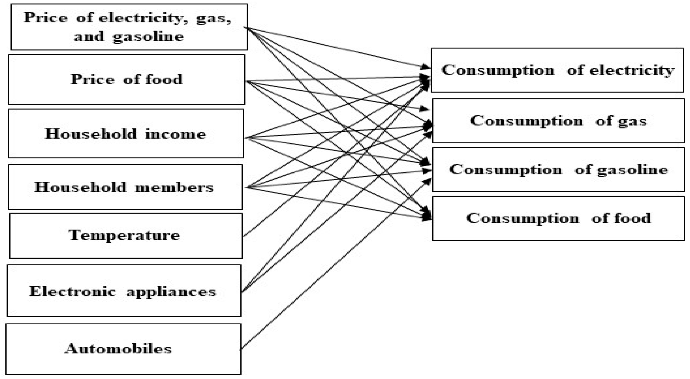
- Dependent variable:
- y1= Electricity, gas, and gasoline consumption
- Independent variables:
- x1 = Price of electricity, gas, and gasoline;
- x2 = Price of other basic goods;
- x3 = Number of household members;
- x4 = Household income;
- x5 = Number of electrical appliances in the home;
- x6 = Number of automobiles per household;
- x7 = Average monthly temperature by state of the republic.
- yi = the dependent variable;
- xi = the i-th element of the matrix of independent variables;
- β = the parameter to be estimated and the slope of the regression line that relates (yi) and (xi);
- u i = the random disturbance that includes all those factors other than the variables xi that influence n yi.
- Model of the Consumption of Electrical Energy:
- Model of the Consumption of Liquefied Petroleum Gas:
- Model of the Consumption of Gasoline:
- Model of the Consumption of Food:
4. Results
5. Discussion
6. Limitation of the Study and Future Research
7. Conclusions
Author Contributions
Funding
Data Availability Statement
Conflicts of Interest
Appendix A
Appendix A.1

| ln (Gas Consumption) | ln (Food Price) | ln (Energy Consumption) | ln (Gasoline Consumption) | ln (Food Consumption) | ln (Gasoline Price) | ln (Energy Price) | ln (Gas Price) | ln (Household Members) | ln (Household Income) | ln (Electrical Appliances) | ln (Temperature) | ln (Automobiles) | |
|---|---|---|---|---|---|---|---|---|---|---|---|---|---|
| Correlation matrix 2012 | |||||||||||||
| ln (gas consumption) | 1 | ||||||||||||
| ln (food Price) | 0.1295 * | 1 | |||||||||||
| ln (energy consumption) | 0.3732 * | 0.0920 * | 1 | ||||||||||
| ln (gasoline consumption) | 0.2265 * | 0.0068 | 0.3180 * | 1 | |||||||||
| ln (food consumption) | 0.2285 * | −0.0735 * | 0.2176 * | 0.2608 * | 1 | ||||||||
| ln (gasoline price) | −0.0004 | 0.0758 * | 0.0567 * | 0.1150 * | 0.0485 * | 1 | |||||||
| ln (energy price) | 0.0646 * | −0.3403 * | −0.1329 * | 0.2170 * | −0.1721 * | 0.0618 * | 1 | ||||||
| ln (gas price) | −0.0363 * | 0.0337 * | −0.0113 | −0.0076 | 0.0179 | −0.0098 | −0.0290 * | 1 | |||||
| ln (household members) | 0.1435 * | 0.2187 * | 0.1374 * | 0.1091 * | 0.1746 * | 0.0032 | −0.0021 | −0.0049 | 1 | ||||
| ln (household income) | 0.3572 * | 0.2679 * | 0.4353 * | 0.5951 * | 0.5015 * | 0.1434 * | 0.2255 * | 0.003 | 0.2563 * | 1 | |||
| ln (electrical appliances) | 0.2385 * | 0.3026 * | 0.2857 * | 0.425 * | 0.2482 * | 0.02434 | 0.1357 * | 0.03761 * | 0.1483 * | 0.4789 * | 1 | ||
| ln (temperature) | −0.2212 * | 0.1673 * | 0.0866 * | 0.0779 * | −0.004 | −0.0096 | −0.2482 * | 0.1563 * | −0.028 | −0.0392 | −0.0366 | 1 | |
| ln (automobiles) | 0.0435 * | 0.0329 * | 0.1856 * | 0.4134 * | 0.1428 | 0.1206 * | 0.1025 * | 0.0287 * | 0.1032 * | 0.3603 * | 0.3147 * | −0.0893 * | 1 |
| Correlation matrix 2014 | |||||||||||||
| ln (gas consumption) | 1 | ||||||||||||
| ln (food Price) | 0.1476 * | 1 | |||||||||||
| ln (energy consumption) | 0.1092 * | 0.1078 * | 1 | ||||||||||
| ln (gasoline consumption) | 0.1059 * | 0.0795 * | 0.2280 * | 1 | |||||||||
| ln (food consumption) | 0.0973 * | −0.0616 * | 0.1417 * | 0.1798 * | 1 | ||||||||
| ln (gasoline price) | −0.0061 | 0.0133 | 0.0009 | −0.0398 * | 0.0093 | 1 | |||||||
| ln (energy price) | 0.0551 * | −0.2543 * | −0.0763 * | 0.1770 * | 0.0791 * | 0.0243 * | 1 | ||||||
| ln (gas price) | −0.2173 * | −0.0231 * | 0.0540 * | 0.0454 * | −0.0411 * | 0.0126 | 0.0247 * | 1 | |||||
| ln (household members) | 0.1287 * | 0.3180 * | 0.0959 * | 0.1032 * | 0.2426 * | −0.0087 | −0.0019 | −0.0227 * | 1 | ||||
| ln (household income) | 0.1644 * | 0.2151 * | 0.2924 * | 0.4745 * | 0.2407 * | 0.0582 * | 0.1886 * | 0.0023 | 0.2201 * | 1 | |||
| ln (electrical appliances) | 0.2217 * | 0.2354 * | 0.3280 * | 0.4045 * | 0.2321 * | 0.0249 * | 0.1399 * | 0.0025 | 0.1157 * | 0.5601 * | 1 | ||
| ln (temperature) | −0.2304 * | 0.1425 * | −0.0854 * | −0.0969 * | −0.0057 | −0.0015 | −0.2118 * | 0.1323 * | −0.0098 | −0.0969 * | −0.0844 * | 1 | |
| ln (automobiles) | 0.0519 * | 0.0599 * | 0.1616 * | 0.4271 * | 0.1320 * | 0.1140 * | 0.1060 * | 0.0412 * | 0.0916 * | 0.3764 * | 0.3020 * | −0.0653 * | 1 |
| Correlation matrix 2016 | |||||||||||||
| ln (gas consumption) | 1 | ||||||||||||
| ln (food Price) | 0.0777 * | 1 | |||||||||||
| ln (energy consumption) | 0.1622 * | 0.1122 * | 1 | ||||||||||
| ln (gasoline consumption) | 0.1684 * | 0.0419 * | 0.2325 * | 1 | |||||||||
| ln (food consumption) | 0.1152 * | −0.1250 * | 0.1509 * | 0.1742 * | 1 | ||||||||
| ln (gasoline price) | 0.0016 | 0.006 | 0.0117 * | −0.0379 * | 0.0120 * | 1 | |||||||
| ln (energy price) | −0.0930 * | 0.2932 * | −0.0863 * | −0.1934 * | −0.0840 * | −0.0224 * | 1 | ||||||
| ln (gas price) | −0.3307 * | −0.1113 * | −0.0984 * | −0.0979 * | −0.0875 * | 0.0096 * | 0.0661 * | 1 | |||||
| ln (household members) | 0.0854 * | 0.3289 * | 0.1283 * | 0.1325 * | 0.2340 * | −0.0009 | −0.0208 * | −0.1330 * | 1 | ||||
| ln (household income) | 0.2802 * | 0.1573 * | 0.2881 * | 0.4461 * | 0.2294 * | 0.0490 * | −0.1910 * | −0.1388 * | 0.2758 * | 1 | |||
| ln (electrical appliances) | 0.2644 * | 0.1603 * | 0.3629 * | 0.3927 * | 0.2222 * | 0.0286 * | −0.1601 * | −0.1783 * | 0.1536 * | 0.5426 * | 1 | ||
| ln (temperature) | −0.1960 * | 0.2283 * | −0.0171 * | −0.1488 * | −0.0673 * | −0.0088 * | 0.3409 * | 0.1856 * | −0.0177 * | −0.1453 * | −0.0971 * | 1 | |
| ln (automobiles) | 0.1068 * | 0.0223 * | 0.1550 * | 0.4057 * | 0.1280 * | 0.1039 * | −0.1146 * | −0.0425 * | 0.1130 * | 0.3451 * | 0.2969 * | −0.0856 * | 1 |
| Correlation matrix 2018 | |||||||||||||
| ln (gas consumption) | 1 | ||||||||||||
| ln (food Price) | 0.1295 * | 1 | |||||||||||
| ln (energy consumption) | 0.1212 * | 0.1147 * | 1 | ||||||||||
| ln (gasoline consumption) | 0.1223 * | 0.0776 * | 0.2432 * | 1 | |||||||||
| ln (food consumption) | 0.0975 * | −0.1079 * | 0.1453 * | 0.1674 * | 1 | ||||||||
| ln (gasoline price) | −0.0131 * | 0.0323 * | 0.009 | −0.0371 * | 0.0149 * | 1 | |||||||
| ln (energy price) | −0.0478 * | 0.2724 * | −0.1212 * | −0.1699 * | −0.0895 * | −0.003 | 1 | ||||||
| ln (gas price) | −0.1244 * | −0.0198 * | 0.0517 * | 0.0461 * | −0.0197 * | 0.0258 * | −0.0228 * | 1 | |||||
| ln (household members) | 0.1548 * | 0.3307 * | 0.1270 * | 0.1581 * | 0.2343 * | 0.0054 | −0.0186 * | −0.0344 * | 1 | ||||
| ln (household income) | 0.1848 * | 0.1865 * | 0.2972 * | 0.4486 * | 0.2354 * | 0.0534 * | −0.1667 * | −0.0206 * | 0.3004 * | 1 | |||
| ln (electrical appliances) | 0.2147 * | 0.1859 * | 0.3575 * | 0.3992 * | 0.2129 * | 0.0188 * | −0.1311 * | 0 | 0.1563 * | 0.5445 * | 1 | ||
| ln (temperature) | −0.2053 * | 0.1915 * | −0.0295 * | −0.1143 * | −0.0559 * | 0.0035 | 0.2857 * | 0.1285 * | −0.0272 * | −0.1352 * | −0.0822 * | 1 | |
| ln (automobiles) | 0.0660 * | 0.0497 * | 0.1610 * | 0.4131 * | 0.1264 * | 0.0758 * | −0.1069 * | 0.0417 * | 0.1329 * | 0.3416 * | 0.3077 * | −0.0677 * | 1 |
Appendix A.2
| Dependent variable: Consumption of Liquefied Petroleum Gas | ||||
| Variable | 2012 | 2014 | 2016 | 2018 |
| ln (household income) | 1.25 | 1.57 | 1.54 | 1.57 |
| ln (electrical appliances) | 1.12 | 1.51 | 1.46 | 1.45 |
| ln (food price) | 1.32 | 1.32 | 1.35 | 1.32 |
| ln (energy price) | 1.29 | 1.19 | 1.27 | 1.22 |
| ln (temperature) | 1.38 | 1.09 | 1.22 | 1.21 |
| ln (household members) | 1.36 | 1.15 | 1.21 | 1.15 |
| ln (liquefied petroleum gas price) | 1.00 | 1.02 | 1.09 | 1.02 |
| ln (gasoline price) | 1.02 | 1.00 | 1.00 | 1.00 |
| Dependent variable: Consumption of Energy | ||||
| Variable | 2012 | 2014 | 2016 | 2018 |
| ln (household income) | 1.25 | 1.57 | 1.54 | 1.57 |
| ln (electrical appliances) | 1.12 | 1.51 | 1.46 | 1.45 |
| ln (food price) | 1.32 | 1.32 | 1.35 | 1.32 |
| ln (energy price) | 1.29 | 1.19 | 1.27 | 1.22 |
| ln (temperature) | 1.38 | 1.09 | 1.22 | 1.21 |
| ln (household members) | 1.36 | 1.15 | 1.21 | 1.15 |
| ln (liquefied petroleum gas price) | 1.00 | 1.02 | 1.09 | 1.02 |
| ln (gasoline price) | 1.02 | 1.00 | 1.00 | 1.00 |
| Dependent variable: Consumption of Gasoline | ||||
| Variable | 2012 | 2014 | 2016 | 2018 |
| ln (household income) | 1.17 | 1.31 | 1.28 | 1.28 |
| ln (automobiles) | 1.32 | 1.18 | 1.15 | 1.14 |
| ln (food price) | 1.38 | 1.26 | 1.29 | 1.27 |
| ln (energy price) | 1.27 | 1.15 | 1.18 | 1.15 |
| ln (household members) | 1.12 | 0.87 | 1.21 | 1.21 |
| ln (liquefied petroleum gas price) | 1.29 | 1.01 | 1.04 | 1.01 |
| ln (gasoline price) | 1.01 | 1.00 | 1.01 | 1.01 |
| Dependent variable: Consumption of Food | ||||
| Variable | 2012 | 2014 | 2016 | 2018 |
| ln (household income) | 1.14 | 1.56 | 1.53 | 1.56 |
| ln (electrical appliances) | 1.24 | 1.50 | 1.46 | 1.45 |
| ln (food price) | 1.40 | 1.30 | 1.30 | 1.29 |
| ln (energy price) | 1.06 | 1.16 | 1.19 | 1.16 |
| ln (household members) | 1.25 | 1.15 | 1.21 | 1.21 |
| ln (liquefied petroleum gas price) | 1.03 | 1.00 | 1.05 | 1.00 |
| ln (gasoline price) | 1.00 | 1.00 | 1.00 | 1.00 |
References
- U.N. General Assembly. Resolution adopted by the General Assembly on 25 September 2015. Transforming our world: The 2030 Agenda for Sustainable Development. 2015. Available online: https://sdgs.un.org/2030agenda (accessed on 26 September 2023).
- U.N. General Assembly. Political Declaration of the High-Level Political Forum on Sustainable Development Convened under the Auspices of the General Assembly, A/RES/74/4. 2019. Available online: https://undocs.org/en/A/RES/74/4 (accessed on 1 August 2023).
- U.N. Economic and Social Council. High-Level Political Forum on Sustainable Development. (A/78/80-E/2923/64). Available online: https://hlpf.un.org/sities/default/2023-06/E%20HLPF%202023%201.PDF (accessed on 10 July 2023).
- Huck, A.; Monstadt, J.; Driessen, P.P.J.; Rudolph-Cleff, A. Towards Resilient Rotterdam? Key conditions for a networked approach to managing urban infrastructure risks. J. Contingencies Crisis Manag. 2021, 29, 12–22. [Google Scholar] [CrossRef]
- Chirisa, I.; Bandauko, E.; Mazhindu, E.; Kwangwama, N.A.; Chikowore, G. Building resilient infrastructure in the face of climate change in African cities: Scope, potentiality, and challenges. Dev. South. Afr. 2016, 33, 113–127. [Google Scholar] [CrossRef]
- Woods, D.D.; Alderson, D.L. Progress toward Resilient Infrastructures: Are We Falling behind the Pace of Events and Changing Threats? J. Crit. Infrastruct. Policy 2021, 2, 5–18. [Google Scholar] [CrossRef]
- Sun, R.; Liu, Y.; Zhao, J. Innovation Network Reconfiguration Makes Infrastructure Megaprojects More Resilient. Comput. Intell. Neurosci. 2022, 2022, 1727030. [Google Scholar] [CrossRef] [PubMed]
- Trinh, V.L.; Chung, C.K. Renewable Energy for SDG-7 and Sustainable Electrical Production, Integration, Industrial Application, and Globalization: Review. Clean. Eng. Technol. 2023, 15, 100657. [Google Scholar] [CrossRef]
- MacArthur, J.L.; Hoicka, C.E.; Castleden, H.; Das, R.; Lieu, J. Canada’s Green New Deal: Forging the Socio-Political Foundations of Climate Resilient Infrastructure? Energy Res. Soc. Sci. 2020, 65, 101442. [Google Scholar] [CrossRef]
- International Energy Agency. International Energy Agency (IEA) World Energy Outlook. 2022, 524. Available online: https://www.Iea.Org/Reports/World-Energy-Outlook-2022/Executive-Summary (accessed on 11 August 2023).
- Paravantis, J.A.; Kontoulis, N. Energy Security and Renewable Energy: A Geopolitical Perspective. In Renewable Energy-Resources, Challenges and Applications; Al Qubeissi, M., El-kharouf, A., Serhad Soyhan, H., Eds.; IntechOpen: London, UK, 2020. [Google Scholar] [CrossRef]
- Strojny, J.; Krakowiak-Bal, A.; Knaga, J.; Kacorzyk, P. Energy Security: A Conceptual Overview. Energies 2023, 16, 5042. [Google Scholar] [CrossRef]
- Jonek-Kowalska, I. Assessing the Energy Security of European Countries in the Resource and Economic Context. Oeconomia Copernic. 2022, 13, 301–334. [Google Scholar] [CrossRef]
- Baker, N.B.; Khater, M.; Haddad, C. Political Stability and the Contribution of Private Investment Commitments in Infrastructure to GDP: An Institutional Perspective. Public Perform. Manag. Rev. 2019, 42, 808–835. [Google Scholar] [CrossRef]
- World Bank. Private Participation in Infrastructure: 2022 Report. 2022. Available online: https://ppi.worldbank.org/content/dam/PPI/documents/PPI-2022-Annual-Report.pdf (accessed on 12 August 2023).
- Alpizar-Castro, I.; Rodríguez-Monroy, C. Review of Mexico’s Energy Reform in 2013: Background, Analysis of the Reform and Reactions. Renew. Sustain. Energy Rev. 2016, 58, 725–736. [Google Scholar] [CrossRef]
- United States Congress House. Pursuing North American Energy Independence: Mexico’s Energy Reforms: Hearing before the Subcommittee on the Western Hemisphere of the Committee on Foreign Affairs, House of Representatives, One Hundred Fourteenth Congress, First Session, 23 July 2015. Available online: https://www.govinfo.gov/content/pkg/CHRG-114hhrg95638/html/CHRG-114hhrg95638.htm (accessed on 12 August 2023).
- International Energy Agency. 2013. Available online: https://www.eia.gov/international/rankings/country/MEX (accessed on 15 August 2023).
- Moshiri, S.; Martínez, M. The welfare effects of energy price changes due to energy market reform in México. Energy Policy 2018, 113, 663–672. [Google Scholar] [CrossRef]
- Clavellina Miller, J.L. Reforma Energética, ¿era Realmente Necesaria? Econ. Inf. 2014, 385, 3–45. [Google Scholar] [CrossRef]
- Balza, L.; Jiménez, R.; Mercado, J. Privatization, Institutional Reform, and Performance in the Latin American Electricity Sector. In Inter-American Development Bank Technical Notes; Inter-American Development Bank: Washington, DC, USA, 2013. [Google Scholar]
- Londoño Pineda, A.A.; Baena Rojas, J.J. Análisis de la relación entre los subsidios al sector energético y algunas variables vinculantes en el desarrollo sostenible en México en el periodo 2004–2010. Gestión y Política Pública 2017, 26, 491–526. [Google Scholar]
- von Moltke, A.; McKee, C.; Morgan TTöpfer, K. Energy Subsidies: Lessons Learned in Assessing Their Impact and Designing Policy Reforms, 1st ed.; Routledge: Sheffield, UK, 2004; Available online: https://search.ebscohost.com/login.aspx?direct=true&AuthType=sso&db=e000xww&AN=525538&lang=es&site=eds-live&scope=site (accessed on 15 August 2023).
- Albatayneh, A.; Juaidi, A.; Manzano-Agugliaro, F. The Negative Impact of Electrical Energy Subsidies on the Energy Consumption—Case Study from Jordan. Energies 2023, 16, 981. [Google Scholar] [CrossRef]
- Jamasb, T.; Nepal, R.; Timilsina, G.R. A Quarter Century Effort Yet to Come of Age: A Survey of Electricity Sector Reform in Developing Countries. Energy J. 2017, 38, 195–234. [Google Scholar] [CrossRef]
- Alberini, A. Household Energy Use, Energy Efficiency, Emissions, and Behaviors. Energy Effic. 2018, 11, 577–588. [Google Scholar] [CrossRef]
- Mankiw, N. Principles of Economics, 6th ed.; Cengage Learning: Boston, MA, USA, 2017. [Google Scholar]
- Chang, B.; Kang, S.J.; Jung, T.Y. Price and Output Elasticities of Energy Demand for Industrial Sectors in OECD Countries. Sustainability 2019, 11, 1786. [Google Scholar] [CrossRef]
- Liddle, B. What Is the Temporal Path of the GDP Elasticity of Energy Consumption in OECD Countries? An Assessment of Previous Findings and New Evidence. Energies 2022, 15, 3802. [Google Scholar] [CrossRef]
- Barten, A.P.; Böhm, V. Consumer Theory. In Handbook of Mathematical Economics; Elsevier: Amsterdam, The Netherlands, 1962; pp. 381–429. [Google Scholar] [CrossRef]
- Chang, Y.; Martinez-Chombo, E.; Electricity Demand Analysis Using Cointegration and Error-Correction Models with Time Varying Parameters: The Mexican Case. Rice University. 2003. Available online: http://www.ruf.rice.edu/~econ/papers/2003papers/08Chang.pdf (accessed on 9 August 2023).
- Galindo, L.M. Short-and long-run demand for energy in Mexico: A cointegration approach. Energy Policy 2005, 33, 1179–1185. [Google Scholar] [CrossRef]
- Sheinbaum-Pardo, C.; Chávez-Baeza, C. Economía de combustible de los autos de pasajeros nuevos en México: Tendencias de 1988 a 2008 y perspectiva. Energy Policy 2011, 39, 8153–8162. [Google Scholar] [CrossRef]
- Sánchez, A.; Islas, S.; Sheinbaum, C. Demanda de gasolina y la heterogeneidad en los ingresos de los hogares en México. Investig. Económica 2015, 74, 117–143. [Google Scholar] [CrossRef]
- Berndt, E.R.; Botero, G. Energy demand in the transportation sector of Mexico. J. Dev. Econ. 1985, 17, 219–238. [Google Scholar] [CrossRef]
- Moshiri, S. The effects of the energy price reform on households’ consumption in Iran. Energy Policy 2015, 79, 177–188. [Google Scholar] [CrossRef]
- ENIGH. National Survey of Household Income and Expenditures 2012. Available online: https://www.inegi.org.mx/programas/enigh/tradicional/2012 (accessed on 11 August 2023).
- ENIGH. National Survey of Household Income and Expenditures 2014. Available online: https://www.inegi.org.mx/programas/enigh/tradicional/2014 (accessed on 12 August 2023).
- ENIGH. National Survey of Household Income and Expenditures 2016. Available online: https://www.inegi.org.mx/programas/enigh/tradicional/2016 (accessed on 12 August 2023).
- ENIGH. National Survey of Household Income and Expenditures 2018. Available online: http://www.inegi.org.mx/programas/enigh/tradicional/2018 (accessed on 13 August 2013).
- Sánchez, B.; y Vicéns, J. Regresión Cuantílica: Estimación y Contraste [Quantile Regression: Estimation and Contrasts]. Instituto L.R. Klein-Centro Gauss. 2012. U.A.M.D.T. No. 21. Available online: https://studylib.es/doc/4656510/regresi%C3%B3n-cuant%C3%ADlica—estimaci%C3%B3n-y-contrastes (accessed on 15 August 2023).
- Hancevic, P.; Navajas, F. Consumo residencial de electricidad y eficiencia energética. El Trimest. Económico 2015, 82, 897–927. [Google Scholar] [CrossRef]
- Heckman, J.J. Sample selection bias as a specification error. Econometrica 1979, 47, 153–161. [Google Scholar] [CrossRef]
- Koenker, R.; Bassett, G., Jr. Regression Quantiles. Econometrica 1978, 46, 33–50. [Google Scholar] [CrossRef]
- Okajima, S.; Okajima, H. Estimation of Japanese Price Elasticities of Residential Electricity Demand, 1990–2007. Energy Econ. 2013, 40, 433–440. [Google Scholar] [CrossRef]
- Pashardes, P.; Pashourtidou, N.; Zachariadis, T. Estimating Welfare Aspects of Changes in Energy Prices from Preference Heterogeneity. Energy Econ. 2014, 42, 58–66. [Google Scholar] [CrossRef]
- Schulte, I.; Heindl, P. Price and Income Elasticities of Residential Energy Demand in Germany. Energy Policy 2017, 102, 512–528. [Google Scholar] [CrossRef]
- INEGI. National Survey on the Consumption of Energy Sources in Private Housing Units (ENCEVI) 2018. Available online: http://en.www.inegi.org.mx/programas/encevi/2018/ (accessed on 15 August 2023).
- León-Bon, T.; Díaz-Bautista, A. Impacto de la inflación de los precios de los alimentos en el bienestar de los hogares en situación de pobreza en México. Rev. Aliment. Contemp. Desarro. Reg. 2020, 30. [Google Scholar] [CrossRef]
- Fernández, L. La Demanda Residencial de Electricidad en ESPAÑA: Un Análisis Microeconométrico. Ph.D. Thesis, Universidad de Barcelona, Barcelona, Spain, 2006. Available online: http://www.tesisenxarxa.net/TDX-0604110-103741/index.html (accessed on 21 March 2022).
- Agostini, C.; Plotter, C.; Saavedra, E. Demanda residencial de energía eléctrica en Chile. Rev. Econ. Chil. 2012, 15, 64–83. [Google Scholar]
- SENER Energy Information System Average Electricity Prices by Tariff Sector. Available online: https://sie.energia.gob.mx/ (accessed on 30 September 2022).
- Federal Electricity Commission. CFE. Available online: http://www.cfe.gob.mx/tarifas/ (accessed on 30 October 2022).
- Obaideen, K.; Olabi, A.G.; Al Swailmeen, Y.; Shehata, N.; Abdelkareem, M.A.; Alami, A.H.; Rodriguez, C.; Sayed, E.T. Solar Energy: Applications, Trends Analysis, Bibliometric Analysis and Research Contribution to Sustainable Development Goals (SDGs). Sustainability 2023, 15, 1418. [Google Scholar] [CrossRef]
- Razzaq, I.; Amjad, M.; Qamar, A.; Asim, M.; Ishfaq, K.; Razzaq, A.; Mawra, K. Reduction in Energy Consumption and CO2 Emissions by Retrofitting an Existing Building to a Net Zero Energy Building for the Implementation of SDGs 7 and 13. Front. Environ. Sci. 2023, 10, 1028793. [Google Scholar] [CrossRef]
- Halkos, G.E.; Tsirivis, A.S. Electricity Prices in the European Union Region: The Role of Renewable Energy Sources, Key Economic Factors and Market Liberalization. Energies 2023, 16, 2540. [Google Scholar] [CrossRef]
- Matin Echeverria, V.; Reyna, B.-R. The Pro-Government Bias as Frame Fidelity. Media Coverage of the 2013 Energy Reform in Mexico. Rev. Mex. Cienc. Políticas Soc. 2013, 62, 229–254. [Google Scholar] [CrossRef]
- Li, Q.; Roh, S.; Lee, J.W. Segmenting the South Korean Public According to Their Preferred Direction for lectricity Mix Reform. Sustainability 2020, 12, 9053. [Google Scholar] [CrossRef]
- Wang, H.; Wang, C.; Zhao, W. Decision on Mixed Trading between Medium- and Long-Term Markets and Spot Markets for Electricity Sales Companies under New Electricity Reform Policies. Energies 2022, 15, 9568. [Google Scholar] [CrossRef]
- Hojati Najafabadi, A.; Rahmati, M.H.; Madanizadeh, S.A. The Dynamic of Discriminatory Reform: How Does Discretionary Pricing Neutralize the Productivity Gains of Energy Subsidy Reform in Iran? J. Appl. Econ. 2023, 26, 2241167. [Google Scholar] [CrossRef]
- Makrygiorgou, J.J.; Karavas, C.S.; Dikaiakos, C.; Moraitis, I.P. The Electricity Market in Greece: Current Status, Identified Challenges, and Arranged Reforms. Sustainability 2023, 15, 3767. [Google Scholar] [CrossRef]
- National Water Commission. Average Temperature by State and National 2012, 2014, 2016 and 2018. Available online: https://www.gob.mx/conagua (accessed on 15 August 2022).
| Year | Households |
|---|---|
| 2012 | 64,246 |
| 2014 | 41,427 |
| 2016 | 82,718 |
| 2018 | 87,826 |
| Variable | 2012 | 2014 | 2016 | 2018 | ||||||||||||
|---|---|---|---|---|---|---|---|---|---|---|---|---|---|---|---|---|
| Mean | Standard Deviation | Pr (Skewness) | Pr (Kurtosis) | Mean | Standard Deviation | Pr (Skewness) | Pr (Kurtosis) | Mean | Standard Deviation | Pr (Skewness) | Pr (Kurtosis) | Mean | Standard Deviation | Pr (Skewness) | Pr (Kurtosis) | |
| ln (gas consumption) | 0.0586 | 0.0067 | 0.0000 | 0.0000 | 0.0365 | 0.0375 | 0.0000 | 0.0000 | 6.1160 | 1.6153 | 0.0000 | 0.0000 | 0.0388 | 0.0386 | 0.0865 | 0.000 |
| ln (food Price) | 3.2447 | 0.6574 | 0.0000 | 0.0000 | 3.1144 | 0.6267 | 0.0000 | 0.0000 | 3.0304 | 0.6873 | 0.0000 | 0.0000 | 3.0298 | 0.6687 | 0.0000 | 0.0000 |
| ln (energy consumption) | 0.0626 | 0.0099 | 0.0000 | 0.0000 | 0.0558 | 0.0250 | 0.0000 | 0.0000 | 0.0518 | 0.0210 | 0.0000 | 0.0000 | 0.0555 | 0.0240 | 0.0000 | 0.0000 |
| ln (gasoline consumption) | 0.0296 | 0.0024 | 0.0000 | 0.0000 | 0.0180 | 0.0143 | 0.0000 | 0.0000 | 0.0265 | 0.0436 | 0.0000 | 0.0000 | 0.0285 | 0.0449 | 0.0000 | 0.0000 |
| ln (food consumption) | 6.5728 | 0.4348 | 0.0000 | 0.0000 | 5.4652 | 0.7168 | 0.0000 | 0.0000 | 5.5593 | 0.7604 | 0.0000 | 0.0000 | 5.6877 | 0.7440 | 0.0000 | 0.0000 |
| ln (gasoline price) | 0.0115 | 0.0761 | 0.0000 | 0.0000 | 0.0175 | 0.0634 | 0.0000 | 0.0000 | 0.0147 | 0.0602 | 0.0000 | 0.0000 | 0.0108 | 0.0580 | 0.0000 | 0.0000 |
| ln (energy price) | 0.1477 | 0.0042 | 0.0000 | 0.0000 | 0.1976 | 0.0587 | 0.0000 | 0.0000 | 0.1808 | 0.0548 | 0.0000 | 0.0000 | 0.3892 | 0.0630 | 0.0000 | 0.0000 |
| ln (gas price) | 0.0074 | 0.0006 | 0.0000 | 0.0000 | 0.0033 | 0.0162 | 0.0000 | 0.0000 | 2.5260 | 2.4322 | 0.0000 | 0.0000 | 0.0025 | 0.0271 | 0.0000 | 0.0000 |
| ln (household members) | 1.2307 | 0.5579 | 0.0000 | 0.0000 | 1.1908 | 0.5543 | 0.0000 | 0.3850 | 1.1582 | 0.5592 | 0.0000 | 0.0000 | 1.1379 | 0.5651 | 0.0000 | 0.0000 |
| ln (household income) | 9.9310 | 1.0031 | 0.0000 | 0.0000 | 10.2361 | 0.7803 | 0.0000 | 0.0000 | 10.3052 | 0.7797 | 0.0000 | 0.0000 | 10.4153 | 0.7817 | 0.4085 | 0.0000 |
| ln (electrical appliances) | 2.0373 | 0.5884 | 0.0000 | 0.0000 | 2.0102 | 0.6159 | 0.0000 | 0.0000 | 2.0473 | 0.5936 | 0.0000 | 0.0000 | 2.0146 | 0.5959 | 0.0000 | 0.0000 |
| ln (temperature) | 3.1262 | 0.1789 | 0.0000 | 0.0000 | 3.1268 | 0.1854 | 0.0000 | 0.0000 | 3.1220 | 0.1924 | 0.0000 | 0.0000 | 3.1152 | 0.1760 | 0.0000 | 0.0000 |
| ln (automobiles) | 0.1028 | 0.2845 | 0.0000 | 0.0000 | 0.1036 | 0.2828 | 0.0000 | 0.0000 | 0.1148 | 0.2986 | 0.0000 | 0.0000 | 0.1248 | 0.3098 | 0.0000 | 0.0000 |
| Year/Variable | 2012 | 2014 | 2016 | 2018 | ||||||||
|---|---|---|---|---|---|---|---|---|---|---|---|---|
| Q25 | Q50 | Q75 | Q25 | Q50 | Q75 | Q25 | Q50 | Q75 | Q25 | Q50 | Q75 | |
| ln energy price | −0.002 | −0.004 * | 0.000 | 0.001 | −0.002 | 0.001 | −0.628 ** | −0.225 ** | −0.636 ** | −0.027 ** | −0.026 ** | −0.028 ** |
| (−0.31) | (−2.29) | (0.07) | (0.39) | (−1.17) | (0.33) | (−4.59) | (−3.25) | (−7.92) | (−18.25) | (−33.72) | (−30.13) | |
| ln liquefied petroleum gas price | 0.003 | −0.004 * | −0.007 ** | 0.063 ** | 0.035 ** | 0.033 ** | −0.023 ** | −0.010 ** | −0.009 ** | 0.025 ** | 0.019 ** | 0.022 ** |
| (0.59) | (−2.08) | (−3.03) | (7.70) | (7.24) | (5.73) | (−12.63) | (−8.30) | (−5.59) | (9.69) | (11.75) | (19.99) | |
| ln gasoline price | −0.013 ** | 0.000 | −0.000 | −0.006 ** | −0.003 ** | −0.001 | −0.157 ** | −0.111 * | −0.083 | −0.008 ** | −0.006 ** | −0.005 ** |
| (−3.17) | (0.12) | (−0.05) | (−3.29) | (−4.15) | (−0.66) | (−3.05) | (−2.43) | (−0.81) | (−5.25) | (−10.99) | (−6.95) | |
| ln food price | 0.003 ** | 0.001 ** | 0.000 | 0.001 ** | 0.000 | −0.000 | 0.048 ** | −0.003 | −0.040 ** | 0.001 ** | 0.000 ** | −0.000 |
| (4.08) | (3.47) | (0.72) | (4.25) | (1.05) | (−0.53) | (3.96) | (−0.54) | (−5.64) | (8.21) | (3.94) | (−0.39) | |
| ln household income | −0.001 | 0.003 ** | 0.004 ** | 0.002 ** | 0.004 ** | 0.005 ** | 0.177 ** | 0.297 ** | 0.398 ** | 0.002 ** | 0.003 ** | 0.004 ** |
| (−1.20) | (16.48) | (16.13) | (13.80) | (23.75) | (26.08) | (15.03) | (48.32) | (51.78) | (16.09) | (48.32) | (51.14) | |
| ln household members | 0.003 ** | 0.002 ** | 0.001 ** | 0.002 ** | 0.002 ** | 0.001 ** | 0.214 ** | 0.135 ** | 0.094 ** | 0.002 ** | 0.001 ** | 0.001 ** |
| (4.15) | (8.10) | (3.51) | (10.12) | (11.06) | (6.18) | (18.77) | (14.26) | (7.47) | (15.29) | (16.72) | (10.36) | |
| ln electrical appliances | 0.022 ** | 0.008 ** | 0.012 ** | 0.011 ** | 0.007 ** | 0.006 ** | 1.113 ** | 0.657 ** | 0.555 ** | 0.012 ** | 0.007 ** | 0.006 ** |
| (16.59) | (26.97) | (29.45) | (23.42) | (45.46) | (26.47) | (35.64) | (61.17) | (82.00) | (32.07) | (51.28) | (56.59) | |
| ln temperature | −0.001 | 0.003 ** | 0.006 ** | −0.003 ** | 0.003 ** | 0.005 ** | 0.514 ** | 0.518 ** | 0.592 ** | 0.005 ** | 0.006 ** | 0.006 ** |
| (−0.76) | (4.23) | (7.43) | (−4.30) | (6.18) | (9.13) | (19.47) | (28.94) | (19.55) | (9.77) | (22.48) | (25.51) | |
| Constant | 0.005 | 0.002 | −0.008 ** | 0.004 | −0.002 | −0.009 ** | −1.166 ** | −0.525 ** | −0.953 ** | −0.003 | 0.002 * | −0.001 |
| (0.86) | (0.67) | (−2.62) | (1.04) | (−1.02) | (−3.70) | (−8.70) | (−6.90) | (−9.67) | (−1.49) | (2.41) | (−0.90) | |
| Pseudo R2 | 0.133 | 0.123 | 0.141 | 0.086 | 0.096 | 0.118 | 0.097 | 0.098 | 0.116 | 0.094 | 0.098 | 0.122 |
| Year/Variable | 2012 | 2014 | 2016 | 2018 | ||||||||
|---|---|---|---|---|---|---|---|---|---|---|---|---|
| Q25 | Q50 | Q75 | Q25 | Q50 | Q75 | Q25 | Q50 | Q75 | Q25 | Q50 | Q75 | |
| ln energy price | −2.29 e−17 | −0.010 | −0.002 | −1.49 e−15 | −9.09 e−06 | 0.010 ** | −5.11 e−13 ** | −3.62 e−13 * | −2.53 e−13 | 2.64 e−15 | −0.001 | 0.005 ** |
| (−0.05) | (−1.08) | (−0.53) | (−1.00) | (−0.01) | (4.21) | (−3.94) | (−2.33) | (−0.00) | (0.46) | (−0.34) | (4.41) | |
| ln liquefied petroleum gas price | −0.766 ** | −0.023 | −0.007 | −2.408 ** | −2.468 ** | −0.087 ** | −0.307 ** | −0.383 ** | −0.456 ** | −1.134 ** | −0.255 ** | −0.022 ** |
| (−32.29) | (−0.45) | (−1.49) | (−2660.64) | (−16.44) | (−14.02) | (−3.8 e+12) | (−1158.52) | (−2872.75) | (−171.10) | (−9.19) | (−10.35) | |
| ln gasoline price | 6.90 e−16 ** | −0.012 | −0.009 * | −1.87 e−16 | −0.001 | −0.001 | −1.86 e−13 ** | −1.38 e−13 | −2.17 e−13 | −3.33 e−15 | −0.048 ** | 0.000 |
| (2.85) | (−0.59) | (−1.97) | (−0.51) | (−0.26) | (−0.52) | (−2.88) | (−1.63) | (−0.00) | (−1.14) | (−14.51) | (0.24) | |
| ln food price | −3.91 e−17 | 0.009 ** | 0.006 ** | 1.97 e−16 | 0.001 | 0.004 ** | 1.33 e−13 ** | 1.24 e−13 ** | 9.91 e−14 | 6.96 e−16 | 0.009 ** | 0.003 ** |
| (−1.55) | (8.34) | (6.13) | (1.87) | (1.61) | (14.03) | (3.97) | (2.85) | (0.00) | (1.92) | (20.36) | (26.82) | |
| ln household income | −8.48 e−17 ** | 0.011 ** | 0.002 ** | 4.55 e−16 ** | 0.001 | 0.002 ** | 6.44 e−14 ** | 8.88 e−14 ** | 1.72 e−14 | −1.88 e−16 | 0.006 ** | 0.003 ** |
| (−3.19) | (14.39) | (4.28) | (5.31) | (1.32) | (9.63) | (3.92) | (5.86) | (0.00) | (−0.57) | (13.47) | (25.13) | |
| ln household members | 1.56 e−17 | 0.003 * | −0.000 | 1.40 e−17 | 0.001 | 0.001 ** | 2.47 e−14 | 9.46 e−14 * | 4.43 e−14 | −5.27 e−16 | 0.010 ** | 0.001 ** |
| (0.77) | (2.13) | (−0.03) | (0.06) | (1.55) | (3.34) | (0.75) | (2.15) | (0.00) | (−0.66) | (15.58) | (9.23) | |
| ln electrical appliances | 1.30 e−16 ** | 0.010 ** | 0.017 ** | −1.14 e−15 ** | 0.001 | 0.008 ** | 1.75 e−15 | −5.14 e−14 | 1.06 e−13 | 3.21 e−16 | 0.011 ** | 0.008 ** |
| (4.68) | (8.51) | (8.46) | (−6.49) | (1.66) | (18.03) | (0.03) | (−0.66) | (0.00) | (0.47) | (22.30) | (34.63) | |
| ln temperature | −1.62 e−16 | −0.078 ** | −0.022 ** | −1.63 e−15 | −0.019 | −0.013 ** | −5.76 e−13 ** | −5.68 e−13 * | −4.67 e−13 | −8.64 e−15 | −0.078 ** | −0.014 ** |
| (−1.52) | (−12.97) | (−9.38) | (−1.47) | (−1.84) | (−17.27) | (−2.86) | (−2.01) | (−0.00) | (−1.60) | (−30.00) | (−46.26) | |
| Constant | 0.006 ** | 0.122 ** | 0.066 ** | 0.016 ** | 0.068 ** | 0.060 ** | 6.364 ** | 6.733 ** | 7.090 ** | 0.007 ** | 0.165 ** | 0.061 ** |
| (31.82) | (5.52) | (18.34) | (2648.37) | (2.58) | (39.32) | (2.4 e +13) | (4181.47) | (3393.76) | (169.42) | (15.74) | (50.25) | |
| Pseudo R2 | 0.025 | 0.159 | 0.068 | 0.208 | 0.224 | 0.038 | 0.406 | 0.502 | 0.287 | 0.089 | 0.144 | 0.040 |
| Year/ Variable | 2012 | 2014 | 2016 | 2018 | ||||||||
|---|---|---|---|---|---|---|---|---|---|---|---|---|
| Q25 | Q50 | Q75 | Q25 | Q50 | Q75 | Q25 | Q50 | Q75 | Q25 | Q50 | Q75 | |
| ln energy price | 6.18 e−16 * | −6.08 e−16 * | 0.012 ** | −3.29 e−16 | 2.18 e−15 | 0.018 ** | −2.47 e−14 | 2.15 e−14 | −0.083 ** | 2.30 e−14 | −0.029 ** | −0.034 ** |
| (2.27) | (−2.22) | (11.56) | (−0.25) | (1.50) | (9.39) | (−1.35) | (1.31) | (−20.33) | (1.92) | (−6.76) | (−16.99) | |
| ln liquefied petroleum gasprice | −1.19 e−16 | 1.13 e−16 | −0.000 | 5.30 e−15 | −2.91 e−15 | 0.018 ** | 6.31 e−16 | −5.15 e−16 | −0.000 ** | −4.17 e−14 ** | 0.034 ** | 0.042 ** |
| (−0.98) | (0.52) | (−0.33) | (1.41) | (−0.88) | (5.17) | (1.62) | (−1.86) | (−15.89) | (−2.77) | (5.20) | (13.77) | |
| ln gasoline price | −0.478 ** | −0.480 ** | −0.006 ** | −1.052 ** | −1.100 ** | −0.011 ** | −3.966 ** | −4.051 ** | −0.029 ** | −0.209 ** | −0.120 ** | −0.030 ** |
| (−8.31) | (−2.67) | (−2.84) | (−27.35) | (−16.87) | (−13.15) | (−25.42) | (−20.81) | (−18.30) | (−6.17) | (−6.54) | (−16.42) | |
| ln food price | 8.95 e−18 | −1.74 e−17 | 0.001 ** | −3.14 e−17 | −8.44 e−17 | 0.000 | 8.34 e−16 | 1.12 e−16 | 0.001 ** | 2.69 e−17 | 0.000 | 0.001 ** |
| (0.80) | (−1.02) | (6.57) | (−0.37) | (−1.00) | (0.19) | (1.00) | (0.16) | (5.54) | (0.07) | (1.50) | (9.49) | |
| ln household income | 9.06 e−17 * | 5.96 e−17 | 0.003 ** | 1.14 e−15 ** | −4.81 e−16 | 0.004 ** | 2.52 e−15 | 9.52 e−16 | 0.017 ** | −8.01 e−15 ** | 0.005 ** | 0.018 ** |
| (2.00) | (1.10) | (32.63) | (3.46) | (−1.84) | (21.27) | (0.98) | (0.29) | (31.96) | (−2.70) | (5.77) | (50.39) | |
| ln household members | 9.24 e−18 | 1.99 e−17 | 0.004 ** | 2.49 e−17 | 2.20 e−16 * | 0.001 ** | −9.94 e−16 | −3.20 e−15 * | 0.002 ** | −1.39 e−15 | −0.000 ** | 0.002 ** |
| (0.94) | (1.76) | (3.61) | (0.19) | (2.06) | (2.90) | (−0.95) | (−2.48) | (6.61) | (−1.50) | (−4.05) | (8.19) | |
| ln automobiles | 0.002 ** | 0.004 | 0.002 ** | 0.008 ** | 0.010 ** | 0.004 ** | 0.017 ** | 0.025 ** | 0.012 ** | 0.079 ** | 0.106 ** | 0.011 ** |
| (2.74) | (1.00) | (13.03) | (9.70) | (6.42) | (12.91) | (5.94) | (5.91) | (44.46) | (92.25) | (44.56) | (43.68) | |
| Constant | 0.007 ** | 0.007 ** | −0.026 ** | 0.017 ** | 0.018 ** | −0.047 ** | 0.055 ** | 0.057 ** | −0.134 ** | −0.009 ** | −0.045 ** | −0.110 ** |
| (8.29) | (2.66) | (−29.13) | (22.08) | (13.77) | (−22.79) | (20.83) | (17.13) | (−20.01) | (−21.77) | (−7.12) | (−28.57) | |
| Pseudo R2 | 0.250 | 0.278 | 0.164 | 0.253 | 0.279 | 0.174 | 0.255 | 0.282 | 0.111 | 0.153 | 0.230 | 0.112 |
| Year/ Variable | 2012 | 2014 | 2016 | 2018 | ||||||||
|---|---|---|---|---|---|---|---|---|---|---|---|---|
| Q25 | Q50 | Q75 | Q25 | Q50 | Q75 | Q25 | Q50 | Q75 | Q25 | Q50 | Q75 | |
| ln energy price | −0.012 | −0.038 | −0.026 | 0.008 | −0.034 | −0.048 | 0.151 ** | 0.073 * | 0.100 * | 0.058 | 0.044 | 0.053 |
| (−0.19) | (−0.48) | (−0.36) | (0.16) | (−0.58) | (−0.69) | (3.57) | (2.44) | (2.23) | (1.94) | (1.13) | (1.47) | |
| ln liquefied petroleum gas price | −0.289 | −0.256 * | −0.132 | −1.893 ** | −1.671 ** | −1.273 ** | −0.009 ** | −0.006 ** | −0.003 ** | −0.525 ** | −0.240 ** | 0.021 |
| (−1.37) | (−2.10) | (−0.99) | (−10.16) | (−9.80) | (−7.48) | (−11.81) | (−8.19) | (−5.24) | (−11.11) | (−3.74) | (0.38) | |
| ln gasoline price | −0.001 | 0.075 | 0.124 ** | 0.069 | 0.046 | 0.005 | 0.066 * | 0.044 | 0.066 * | 0.070 ** | 0.064 ** | 0.028 |
| (−0.01) | (0.83) | (2.58) | (1.84) | (0.85) | (0.10) | (2.23) | (1.50) | (2.36) | (2.76) | (3.34) | (1.05) | |
| ln food price | −0.113 ** | −0.174 ** | −0.258 ** | −0.103 ** | −0.169 ** | −0.250 ** | −0.118 ** | −0.189 ** | −0.280 ** | −0.114 ** | −0.182 ** | −0.271 ** |
| (−15.18) | (−15.95) | (−24.23) | (−12.83) | (−20.27) | (−34.24) | (−33.15) | (−50.53) | (−74.03) | (−29.05) | (−40.67) | (−50.92) | |
| ln household income | 0.119 ** | 0.160 ** | 0.181 ** | 0.148 ** | 0.184 ** | 0.201 ** | 0.139 ** | 0.170 ** | 0.187 ** | 0.136 ** | 0.167 ** | 0.190 ** |
| (12.82) | (20.84) | (31.92) | (30.12) | (42.42) | (60.10) | (39.69) | (47.91) | (74.60) | (72.92) | (79.66) | (54.29) | |
| ln household members | 0.244 ** | 0.193 ** | 0.181 ** | 0.205 ** | 0.172 ** | 0.162 ** | 0.206 ** | 0.174 ** | 0.154 ** | 0.206 ** | 0.181 ** | 0.165 ** |
| (23.72) | (25.28) | (20.95) | (36.28) | (22.26) | (25.62) | (56.80) | (50.09) | (39.07) | (53.67) | (66.74) | (61.70) | |
| ln electrical appliances | 0.124 ** | 0.087 ** | 0.072 ** | 0.145 ** | 0.116 ** | 0.099 ** | 0.139 ** | 0.118 ** | 0.111 ** | 0.129 ** | 0.113 ** | 0.097 ** |
| (8.06) | (7.38) | (6.48) | (17.08) | (17.59) | (14.20) | (27.11) | (29.67) | (24.52) | (33.78) | (33.57) | (27.25) | |
| Constant | 4.082 ** | 4.166 ** | 4.426 ** | 3.570 ** | 3.736 ** | 4.094 ** | 3.833 ** | 4.023 ** | 4.400 ** | 3.915 ** | 4.096 ** | 4.413 ** |
| (39.32) | (43.87) | (46.16) | (85.58) | (80.22) | (92.23) | (121.67) | (148.79) | (146.01) | (165.41) | (186.91) | (157.69) | |
| Pseudo R2 | 0.099 | 0.115 | 0.134 | 0.115 | 0.128 | 0.149 | 0.104 | 0.121 | 0.150 | 0.105 | 0.120 | 0.144 |
| Electricity | L.P. GAS | Gasoline | Foods | ||
|---|---|---|---|---|---|
| 2012 | Q25 | −0.002 | −0.766 ** | −0.478 ** | −0.113 ** |
| Q50 | −0.004 * | −0.023 | −0.480 ** | −0.174 ** | |
| Q75 | 0.000 | −0.007 | −0.006 ** | −0.258 ** | |
| 2014 | Q25 | 0.001 | −2.408 ** | −1.052 ** | −0.103 ** |
| Q50 | −0.002 | −2.468 ** | −1.100 ** | −0.169 ** | |
| Q75 | 0.001 | −0.087 ** | −0.011 ** | −0.250 ** | |
| 2016 | Q25 | −0.626 ** | −0.307 ** | −3.966 ** | −0.118 ** |
| Q50 | −0.225 ** | −0.383 ** | −4.051 ** | −0.189 ** | |
| Q75 | −0.636 ** | −0.456 ** | −0.029 ** | −0.280 ** | |
| 2018 | Q25 | −0.027 ** | −1.134 ** | −0.209 ** | −0.114 ** |
| Q50 | −0.026 ** | −0.255 ** | −0.120 ** | −0.182 ** | |
| Q75 | −0.028 ** | −0.022 ** | −0.030 ** | −0.271 ** |
Disclaimer/Publisher’s Note: The statements, opinions and data contained in all publications are solely those of the individual author(s) and contributor(s) and not of MDPI and/or the editor(s). MDPI and/or the editor(s) disclaim responsibility for any injury to people or property resulting from any ideas, methods, instructions or products referred to in the content. |
© 2023 by the authors. Licensee MDPI, Basel, Switzerland. This article is an open access article distributed under the terms and conditions of the Creative Commons Attribution (CC BY) license (https://creativecommons.org/licenses/by/4.0/).
Share and Cite
Garcia-Garza, M.G.; Ortiz-Rodriguez, J.; Picazzo-Palencia, E.; Munguia, N.; Velazquez, L. The 2013 Mexican Energy Reform in the Context of Sustainable Development Goal 7. Energies 2023, 16, 6920. https://doi.org/10.3390/en16196920
Garcia-Garza MG, Ortiz-Rodriguez J, Picazzo-Palencia E, Munguia N, Velazquez L. The 2013 Mexican Energy Reform in the Context of Sustainable Development Goal 7. Energies. 2023; 16(19):6920. https://doi.org/10.3390/en16196920
Chicago/Turabian StyleGarcia-Garza, Maria Guadalupe, Jeyle Ortiz-Rodriguez, Esteban Picazzo-Palencia, Nora Munguia, and Luis Velazquez. 2023. "The 2013 Mexican Energy Reform in the Context of Sustainable Development Goal 7" Energies 16, no. 19: 6920. https://doi.org/10.3390/en16196920
APA StyleGarcia-Garza, M. G., Ortiz-Rodriguez, J., Picazzo-Palencia, E., Munguia, N., & Velazquez, L. (2023). The 2013 Mexican Energy Reform in the Context of Sustainable Development Goal 7. Energies, 16(19), 6920. https://doi.org/10.3390/en16196920