Numerical Analysis of the Differential Flowmeter: Standard Orifice and Slotted Orifices

Abstract

The paper presents the results of simulation studies of fluid flow through a standard orifice and two slotted orifices. The research that has been carried out concerns the analysis of the effect of the orifice geometry on the velocity profiles, turbulence kinetic energy and turbulence energy dispersion. The profile studies were conducted at different distances behind the orifice so that the results could be compared with each other. The studied flow included an airflow whose inlet velocity was 15 m/s. The turbulence model k-ε was used for numerical calculations. The tested orifices were characterized by an orifice constriction equal to β = 0.5. The calculations involved flow through a pipeline with a diameter of 160 mm. The results show that for a standard orifice, the maximum velocity of the flow is about 95 m/s and this is recorded at a distance of about 10–20 cm behind the orifice, and then it decreases, and at a distance of about 60 cm, the flow velocity is about 27 m/s. In the case of slotted holes, the maximum velocity is about 30% lower compared to the flow rate through a standard orifice design. The maximum velocity behind slotted orifices occurs directly behind the orifice, and in the cases of slotted orifice 1 and slotted orifice 2, was about 70 m/s and 67 m/s, respectively. For slotted orifice 1, at a distance of 20 cm behind the orifice, the flow assumed a velocity of about 19 m/s, whereas for slotted orifice 2, the flow reached a speed of about 18 m/s, at a distance of about 30 cm behind the orifice. The values of the maximum kinetic energy of turbulence for the tested orifices are about 420 m²/s² for the standard orifice, and about 250 m²/s² and 220 m²/s² for slotted orifices 1 and 2, respectively. The obtained simulation results demonstrated that slotted orifices lead to faster stream homogenization and do not disturb the flow as much as a standard orifice. Slotted orifices exhibit a higher flow coefficient.

1. Introduction

Fluid flow measurements in a closed conduit are often combined with flow visualization and thus take a special place among the many types of measurements found in industrial and laboratory practice. There is a general lack of universal measurement methods, which are derived from the theoretical principles of operation and the technical feasibility of their application. The variety of conditions in which fluid flow measurements are carried out and the requirements that are placed on the measurement itself lead to the need to search for newer and improved methods in the sense of the range of applications, accuracy requirements and reliability [1,2,3].

Fluid flow measurements play a very important role in areas related to the operation of both individual processes and entire systems. Measurements are used, among others, to control technological processes, the distribution of energy carriers, or often form the basis of settlement [1,4].

The number of different methods available for measuring fluid flow is related to the use of different physical phenomena that accompany flow. Various types of flow devices appear on the market that use unprecedented or rare measurement techniques, and the selection of a suitable method for measuring the flow rate of a flowing fluid is linked to the possession of the appropriate knowledge and experience. The use of suitable flow devices is associated with various measurement problems. The selection of a suitable type of flow meter requires knowledge of much data related to both the nature of the flow, in particular its dynamics, the type of fluid, its physical parameters, their range of variation, as well as the range of the variable fluid flow. The requirements applicable for measurement accuracy and data related to the installation in which the flow meter is to be located also form a challenge [3].

In general, mass flow measurement is extremely important in many industries, and the accuracy of the measurement carried out is of great importance, not least because of rising energy prices [5]. The importance of accurate fluid flow measurement is crucial in industries such as power generation, environmental engineering, oil and gas, mineral processing, petrochemical, chemical industries. Fluid flow measurement can also be encountered in such scientific fields as meteorology and biology. A distinction is made between single-phase flows such as the flow of liquids, gas or solids, such as in the food or cement industry, and multiphase flows (oil, natural gas), sludge flow. Thus, flow measurement includes the flow of compressible as well as incompressible fluids. Various types of flow meters can be used to measure the flow rate, and they can be designed for specific applications, and for this purpose we can mention, for example, flow meters: ultrasonic, electromagnetic, vortex, optical (using the Doppler effect); and mass flow meters [6,7,8,9]. The presented group of instruments is characterized by having a more complicated structure or by its operating principle. Not infrequently, one impediment is related to their calibration. Flowmeters are characterized by sensitivity to deformation of the velocity profile, difficulty in estimating the accuracy of the flow, and in some cases the possibility of measuring in a fluid with a temperature of up to 200 °C. Poor anti-interference capability, short life of the flow meter or high sensitivity to flow disturbances are other disadvantages that the above presented group of flow meters can exhibit. In the event of failure of the flow device when cleaning is required, this can be very difficult or even impracticable. Some of the flow meters are only suitable for specific liquids, making them unsuitable for use in the petrochemical industry or during oil transportation, for example [10]. A major disadvantage is also the high cost of the flow meter. In measurement practice, therefore, there is a great demand for instruments with a simple design and low production cost. In addition, high requirements are placed on the equipment in terms of: reliability, accuracy, repeatability and application range. Therefore, it is reasonable to look for a solution that combines a simple design and provides ease of measurement, high measurement accuracy, low production cost and simple maintenance [11,12]. A flowmeter that meets these criteria is a differential pressure flowmeter.

Considering the qualities outlined above, differential pressure flowmeters in industrial applications are some of the most common instruments of choice for measuring fluid flow rate. Differential pressure flowmeters are very universal because they are suitable for measuring both liquid, gas, slurry and steam, and in a narrow range can even be applied for measuring gas-particulate [3,13]. The range of applications of differential pressure flowmeters includes a wide range of temperatures and pressures. Differential pressure flowmeters, among which we distinguish standard orifices, Venturi tube and nozzles, are some of the oldest, simplest and cheapest methods of flow rate measurement. The basic element which is installed inside the pipe leads to a local reduction in the cross-section of the pipeline. This leads to a narrowing of the stream of the fluid flow, which causes an increase in velocity at the point of narrowing and in turn translates into a change in static pressure. The resulting pressure difference upstream and downstream of the flow constriction element, combined with the differential pressure transducer, is the basis for calculating the mass flow of the flowing fluid, Equation (1) [14,15].

$$\mathrm{m}=\frac{\mathrm{C}}{\sqrt{1-{\mathsf{\beta }}^4}}\mathsf{\epsilon }{\mathrm{A}}_0\sqrt{2\mathsf{\rho }∆\mathrm{p}}$$

(1)

where C—discharge coefficient, β—beta ratio, ε—number of expansion, A₀—cross-sectional area of the hole, ρ—density of the flowing medium, Δp—differential pressure.

Universality forms the main factor behind the widespread use of differential pressure flowmeters, and they are most often used in the energy industry in such measurements as the measurement of boiler water, steam with critical parameters and pressures reaching up to 280 bar and temperatures over 600 °C. In the oil industry, differential pressure flow meters are used at practically every stage of production processing, transportation, storage, refining, and distribution. Differential pressure flowmeters are used for both liquid petroleum products and natural gas. DP flowmeters are also used in the chemical industry for measuring organic and inorganic compounds, basic chemicals, polymers, and fertilizers [8,9,15,16].

Orifice flowmeters are very popular flow measurement instruments due to their advantages, which include: simple design, no moving parts, low manufacturing cost, easy replacement of the orifice without the need to disassemble large measuring sections. Despite these advantages, differential pressure flowmeters have a fundamental disadvantage, which includes low pressure recovery [15,17,18,19]. Another problem is related to the phenomenon of cavitation, which can be observed, among others, in constrictions such as valve slots, when flowing around hydraulic profiles, as well as in orifices or Venturi nozzles [20]. The occurrence of cavitation in the flow produces noise and vibrations in the system. Cavitation also has a negative impact on the operation of hydraulic systems [21]. Due to the popular use of the standard orifice in industry, research has been carried out for years on the use of orifices whose bore shape is different from the standard one, i.e., one that comprises a single circular hole in the central part. In the literature, one can find modifications regarding the orifice opening; these are slotted, multi-hole, fractal orifices. In such orifices, a single hole is replaced by several holes. Orifice solutions in which a single circular hole has been replaced by a single hole in the shape of a square, triangle, oval are also encountered in several studies [22,23,24,25].

Thus, with differential pressure flowmeters, it is necessary to conduct research that considers the metrological properties of orifices with other hole shapes than the standard one.

For such in-depth analysis, one can successfully use numerical methods which, over the past few years, have been widely used in various issues, such as flow simulation. In addition, the physical complexity of flow problems causes difficulties in the mathematical treatment of these processes. Hence, experimental studies and mathematical modeling of flow play such a large role.

Numerical methods are widely used in solving technical problems and allow a result to be obtained that cannot be solved by analytical means or where the solution is too complex and time-consuming. The use of simulations for flow studies is mainly related to the high efficiency and accuracy of numerical fluid mechanics [19]. The use of numerical methods makes it possible to significantly reduce the time needed for ongoing research concerned with the optimization of, for example, a given design solution, and at the stage of creating new products, numerical methods are used as a tool to reduce product development time. Programs that allow numerical studies enable solutions to be obtained to many flow issues, giving a better understanding of the phenomena during the flow of single and multiphase flumes. Numerical methods provide the means for the modeling of turbulence, heat transfer and combustion, ending with chemical reactions [19,26,27,28].

With regard to differential pressure flowmeters, one can find works in which numerical and experimental studies were investigated. The types of analysis conducted for these purposes involve orifices with different geometries, numbers and arrangements of holes. It turns out, for example, that the number or arrangement of holes in multi-hole orifices has a significant impact on the metrological properties of these orifices. A study reported in [29] shows that the constant pressure drop in the multi-hole orifices explored was smaller compared to a standard orifice. However, in some solutions, depending on the number of orifices, the drop was smaller or closer to the drop that was obtained for the standard orifice. Another interesting finding of this study was that one of the solutions of the multi-hole orifice that the authors of the article studied had better properties in terms of flow mixing compared to the other solutions whereas the same design solution was less good in terms of constant pressure drop.

In [24], Golijanek-Jędrzejczyk et al., a numerical and experimental investigation was carried out for a multi-hole orifice in the area of developing turbulent flow. The purpose of the study was to validate the design by comparing numerical study with the experiment conducted in the area of turbulent flow in the range of Reynolds numbers from 4200 to 19,000. The conclusions of the study included that the use of a multi-hole orifice makes it possible to reduce the length of the pipeline sections upstream and downstream of the orifice. Multi-hole orifices demonstrate better metrological properties compared to the standard orifice. Multi-hole orifices are characterized by a regular value of the flow coefficient (the value of this coefficient is higher by about 2% compared to a standard orifice). The research that the authors present was conducted for Reynolds numbers Re > 10.000. Shaaban [30] conducted a study on optimizing the geometry in a multi-hole orifice. The research was conducted using numerical methods. The research involved changing the hole geometry by changing the flow angle at the inlet and outlet of the hole. The conclusions of this research are that due to the change in angle, the pressure drop across the hole was reduced by about 50%, and the flow rate improved by about 15%.

The authors in [5] presented the results of a simulation study of a single-hole SHO orifice and a multi-hole MHO orifice, with different β-factors (0.5, 0.55, 0.6 and 0.7). The fluid tested was air, and the flow involved a wide range of Re numbers. Pressure loss coefficient, flow patterns and pressure recovery were analyzed. Visualization results using computational fluid dynamics derived from simulations were compared with experimental results and suitable agreement was obtained. Experimental results showed that a faster pressure recovery was registered for the MHO orifice compared to the SHO, and the increase in pressure recovery was correlated with an increase in β. The results presented demonstrated the advantages of MHOs over SHOs in terms of specific loss ratio and pressure recovery.

In one paper, reference [19], CFD simulations were conducted with the aim of optimizing the placement of holes in a multi-hole orifice. The results of different configurations of a multi-hole orifice flow meter were compared with computational fluid dynamics visualization results by applying an equivalent single-hole orifice flow meter. In the reported study, the author showed that the discharge coefficient of multi-hole orifices is higher than that of single-hole orifices over a wide range of Reynolds numbers.

In study [31], the research was concerned with the optimization of a single-hole orifice with the purpose of achieving low cavitation. Zhang et al. proposed a solution where a single orifice hole was replaced with a convergent-flat-divergent hole. The focus in the study was on the analysis of the effect of geometric parameters and temperature on the cavitation behavior of the tested orifices. It was found that the convergence angle of the single-hole orifice was an important parameter affecting cavitation. The inlet pressure for both optimized orifices was much lower compared to the original design. The analysis of the effect of temperature on cavitation allowed the authors to conclude that for a constant Reynolds number, fluid viscosity forms a key parameter that determines the conditions of cavitation during variations in temperature, and the values of the cavitation indices decrease with an increase in temperature. For a constant fluid velocity, the cavitation index values increase monotonically following an increase in temperature. Under a constant Reynolds number, the viscosity of the fluid forms the key parameter that determines cavitation in the conditions of variable temperature, and the cavitation index values decrease with an increase in temperature. In the case of a constant fluid velocity, the cavitation indices increase monotonically with increasing temperature. In the literature, we found numerical studies for multi-hole orifices in which velocity profiles, kinetic energy profiles, among other things, were extensively analyzed, but still very little similar analysis could be found for a slotted orifice.

The purpose of this paper is to estimate the metrological properties of a design solution for slotted orifices with a constriction ratio of 0.5.

The novelty element of the research presented in the paper involved the use of a numerical method for the analysis of the resulting flow velocity through the various design solutions of slotted orifices. In addition, the resulting pressure and turbulence kinetic energy characteristics, turbulence energy dissipation rate and velocity profiles formed behind the orifice were analyzed.

2. Materials and Methods

The research was conducted using the method of computational fluid mechanics.

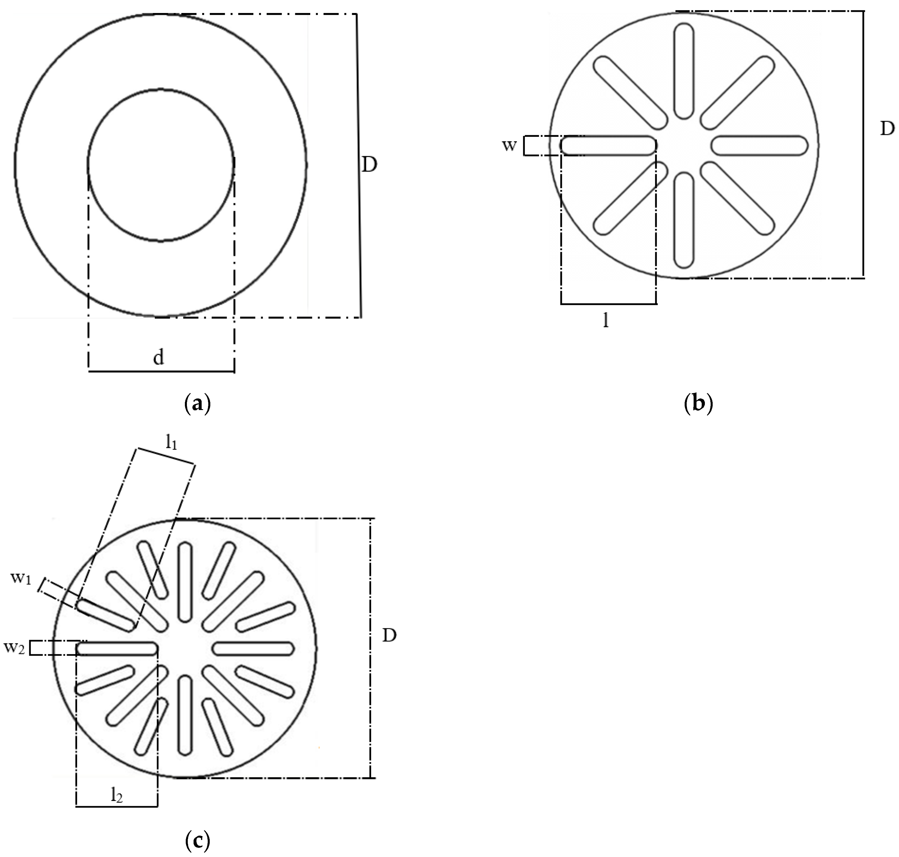
The simulation results present a comparison of a standard orifice and two slotted orifices that differed in geometry and hole location. The geometries of these orifices are shown in Figure 1.

In addition, the geometric dimensions of each orifice are shown in

Table 1. Dimensions of orifice holes.

Orifice	Outside Diameter (D) (mm)	Hole Diameter (d) (mm)	Slot Width (w) (mm)	Slot Length (l) (mm)	Number of Slots
Standard	160	80	-	-	-
Slotted 1	160	-	11.5	57.1	8
Slotted 2			(w1) 7 (smaller slots)	(l1) 36.6 (smaller slots)	8 (smaller slots)
	160	-	(w2) 8 (bigger slots)	(l2) 49.5 (bigger slots)	8 (bigger slots)

.

The dimensions of the holes in the slotted orifices had to be selected in such a way that it would be possible to compare the results obtained for the slotted orifices with those gained for the standard orifice. The dimensions of the slots were chosen so that the square root of the ratio of the total cross-sectional area of the hole to the cross-sectional area of the pipe in all orifices was the same.

$$\mathsf{\beta }=\sqrt{\frac{{\mathrm{A}}_{\mathrm{s}\mathrm{l}\mathrm{o}\mathrm{t}\mathrm{s}}}{{\mathrm{A}}_{\mathrm{p}\mathrm{i}\mathrm{p}\mathrm{e}}}}$$

where A_slots—cross-sectional area of all slots, A_pipe—cross-sectional area of the pipeline.

The constriction of the analyzed orifices was β = 0.5.

The procedure of numerical flow modeling consisted of three steps. The first step involved the development of the computational geometry. The next step was to discretize it, that is, to divide the computational area into smaller elements. The finite volume method was used for simulation calculations. This technique is based on volume control, which transforms the governing equations into algebraic equations that can then be solved numerically. Discretization forms a crucial step because the length of the calculations and the accuracy of the obtained results depend on it. It can be concluded that the greater the number of grid elements, the greater the accuracy of the calculations carried out. However, it should be remembered that by increasing the grid density, we also increase the time scale for the calculations carried out, and a certain degree of density in the grid is sufficient to calculate the issue; further compaction of the grid does not significantly affect the final result, but only increases the calculation time.

2.1. Mesh Grid

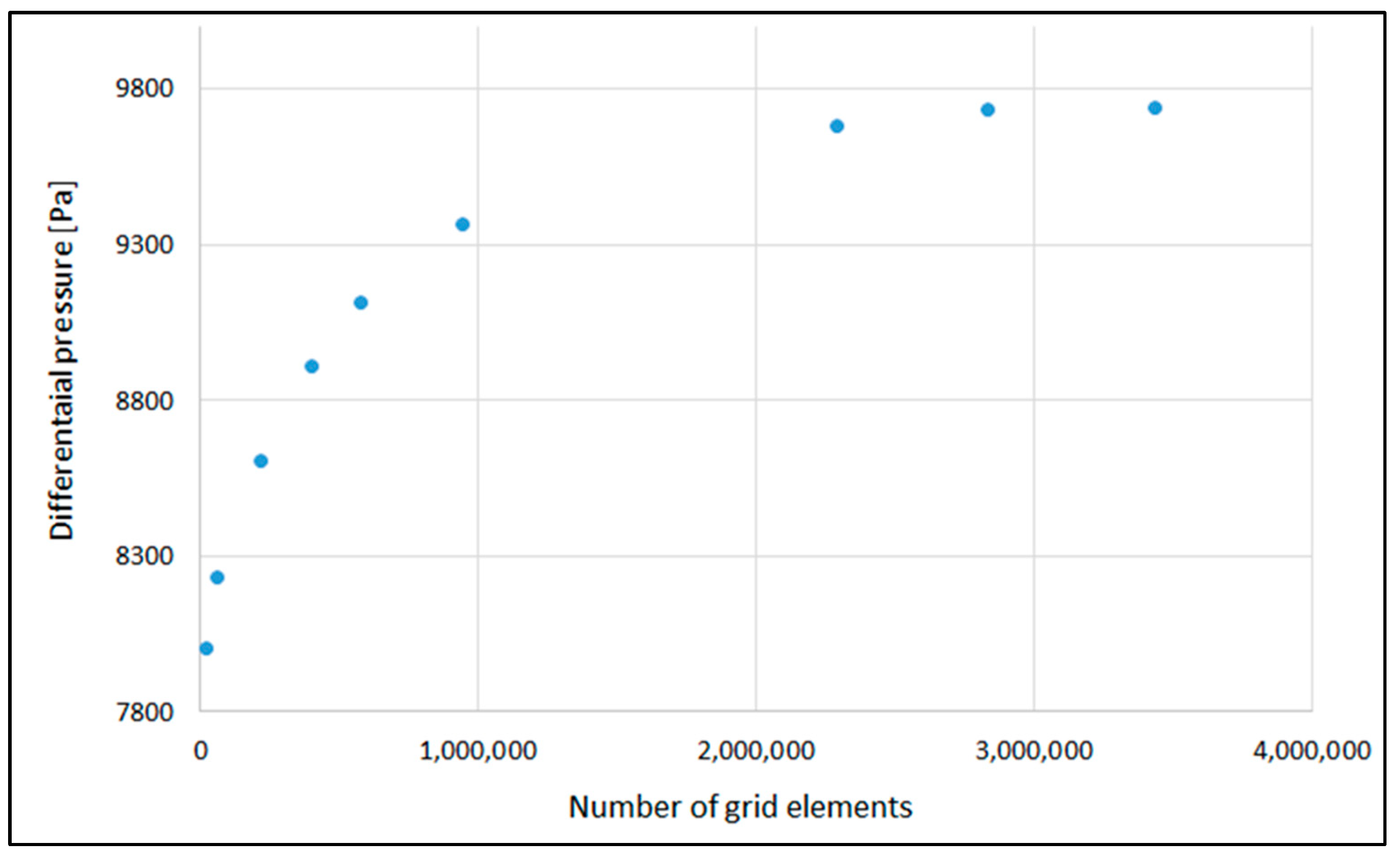
Before proceeding to the relevant numerical calculations, tests were carried out on the influence of mesh density on the results of the modeled calculations. Test calculations were performed for nine grids with different numbers of elements. This analysis concerned the flow of fluid through a standard orifice. The results of these calculations are presented below in graphical form in Figure 2.

Figure 2 shows the results of the analysis of the influence of the number of grid elements on the resulting pressure difference at the orifice.

By analyzing Figure 2, we can see that as the number of grid elements increased, the differential pressure increased, but after crossing a certain limit, this pressure began to stabilize and there was no further need to increase the number of grid elements. It also did not significantly change the velocity and pressure profile, but only increased the time scale of the calculations. Further calculations were carried out for a geometry whose mesh was divided into 2,833,387 elements.

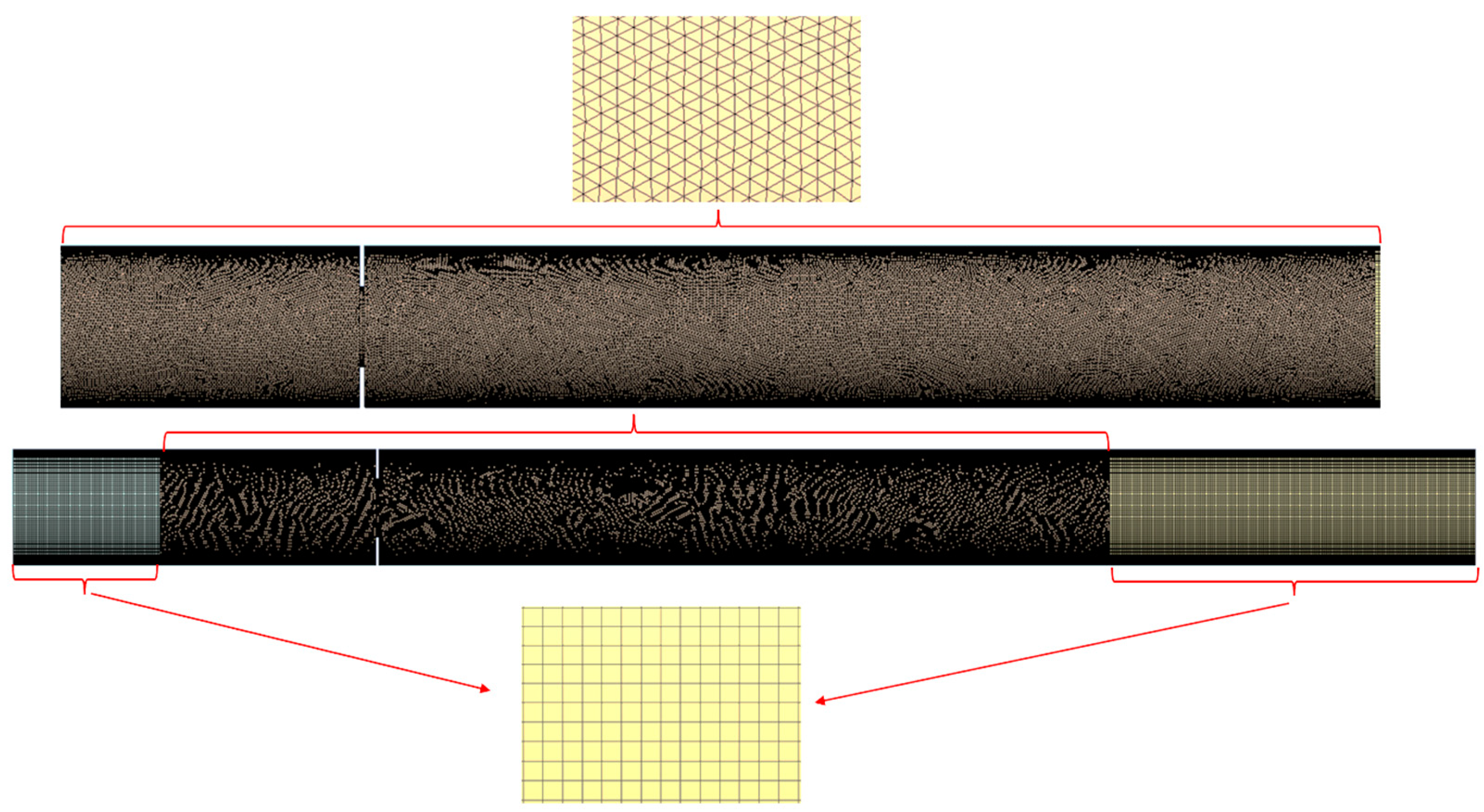
Figure 3 shows the computational grid used in the study. A hybrid grid was used, which was a combination of a structured and unstructured grid. Such division of the computational area made it possible, first of all, to significantly reduce the time scale of the calculations carried out without risking the loss of accuracy of the obtained results. The area was divided in such a way that in places where not much happened, the structural grid was used, and in the areas of the greatest disturbance and the area of potential impact of the applied orifice, the unstructured grid was used.

The third step involved the calculation of the flow domain, after initially determining the turbulence model and setting boundary conditions. Once the solution had converged, the results could be processed and analyzed.

2.2. Governing Equations

Accurate simulation of turbulent flow requires very large computational power. Therefore, the most common engineering approach is to try to average the Navier–Stokes (RANS) equations as a function of time. Since the N–S equations are nonlinear, any averaging process leads to additional unknowns that must be related in some way to the average quantities. In such a case, we can mention the closure of N–S equations in the problem. At this stage, we have to face the so-called turbulence modeling. One of the proposals for such a model is the introduction of new variables and, here, we can define the model: k-ε where k is the kinetic energy of turbulence, ε it is a dispersion of energy. The k-ε model is the simplest and commonly used model in simulations of flow through orifices [4].

The movement of fluid is described by the flow continuity equation and the equation of momentum:

$$\frac{\partial }{\partial \mathrm{t}}\left(\mathsf{\rho }\mathrm{k}\right)+\frac{\partial }{\partial {\mathrm{x}}_{\mathrm{i}}}\left(\mathsf{\rho }\mathrm{k}{\mathsf{\nu }}_{\mathrm{i}}\right)=\frac{\partial }{\partial {\mathrm{x}}_{\mathrm{j}}}\left[\left(\mathsf{\mu }+\frac{{\mathsf{\mu }}_{\mathrm{t}}}{{\mathsf{\sigma }}_{\mathrm{k}}}\right)\frac{\partial \mathrm{k}}{\partial {\mathrm{x}}_{\mathrm{j}}}\right]+{\mathrm{G}}_{\mathrm{k}}-\mathsf{\rho }\mathsf{\epsilon },$$

(2)

$$\frac{\partial }{\partial \mathrm{t}}\left(\mathsf{\rho }\mathsf{\epsilon }\right)+\frac{\partial }{\partial {\mathrm{x}}_{\mathrm{i}}}\left(\mathsf{\rho }\mathsf{\epsilon }{\mathsf{\nu }}_{\mathrm{i}}\right)=\frac{\partial }{\partial {\mathrm{x}}_{\mathrm{j}}}\left[\left(\mathsf{\mu }+\frac{{\mathsf{\mu }}_{\mathrm{t}}}{{\mathsf{\sigma }}_{\mathsf{\epsilon }}}\right)\frac{\partial \mathsf{\epsilon }}{\partial {\mathrm{x}}_{\mathrm{j}}}\right]+{\mathrm{G}}_{1\mathsf{\epsilon }}\frac{\mathsf{\epsilon }}{\mathrm{k}}{\mathrm{G}}_{\mathrm{k}}-{\mathrm{C}}_{2\mathsf{\epsilon }}\mathsf{\rho }\frac{{\mathsf{\epsilon }}^2}{\mathrm{k}}$$

(3)

In the equations above, k is the turbulence kinetic energy, ε is the turbulence energy dissipation rate, and C_1ε, C_2ε are empirical constants, σ_k and σ_ε are the turbulent Prandtl numbers for k and ε, and are, respectively, 1.44, 1.92, 1.00 and 1.3; μ_t is the turbulent viscosity constant and is 0.09. G_k is related to the generation of turbulence kinetic energy, which is caused by viscous and buoyancy forces.

After determining the turbulence model, the boundary conditions had to be determined. Numerical simulations were carried out for a steady-state, compressible, turbulent fluid flow with a Reynolds number of about 79,880. The flow included an air stream with a density of 1.2 kg/m³, and a viscosity coefficient = 1.7894 × 10⁻⁵ kg/(ms). The gas velocity at the inlet was 15 m/s.

The governing equations were numerically solved by the finite volume technique. A SIMPLE scheme was used for pressure–velocity coupling. The gradients were estimated using the least squares cell-based method. The second order upwind scheme and the standard second order scheme were used to discretize momentum and pressure. Turbulence kinetic energy and kinetic energy dissipation rate were discretized using the first order upwind method. A value of 10⁻³ was used as the convergence criterion for the continuity and momentum equations.

Simulation studies were conducted using ANSYS Fluent 2022 software (Ansys Company Inc., Canonsburg, PA, USA). The governing equations were solved based on the finite volume method.

3. Results and Discussion

The results of the simulation studies conducted for standard orifice and slotted orifices are presented below. The results of the flow visualization presented here concern the comparison of pressure distribution and velocity distribution in the pipeline axis. Also compared are velocity profiles at various distances behind the orifice and velocity contours and velocity vectors for different design solutions of the orifice geometry and axial profiles at various distances behind the orifice of the coefficient k and ε.

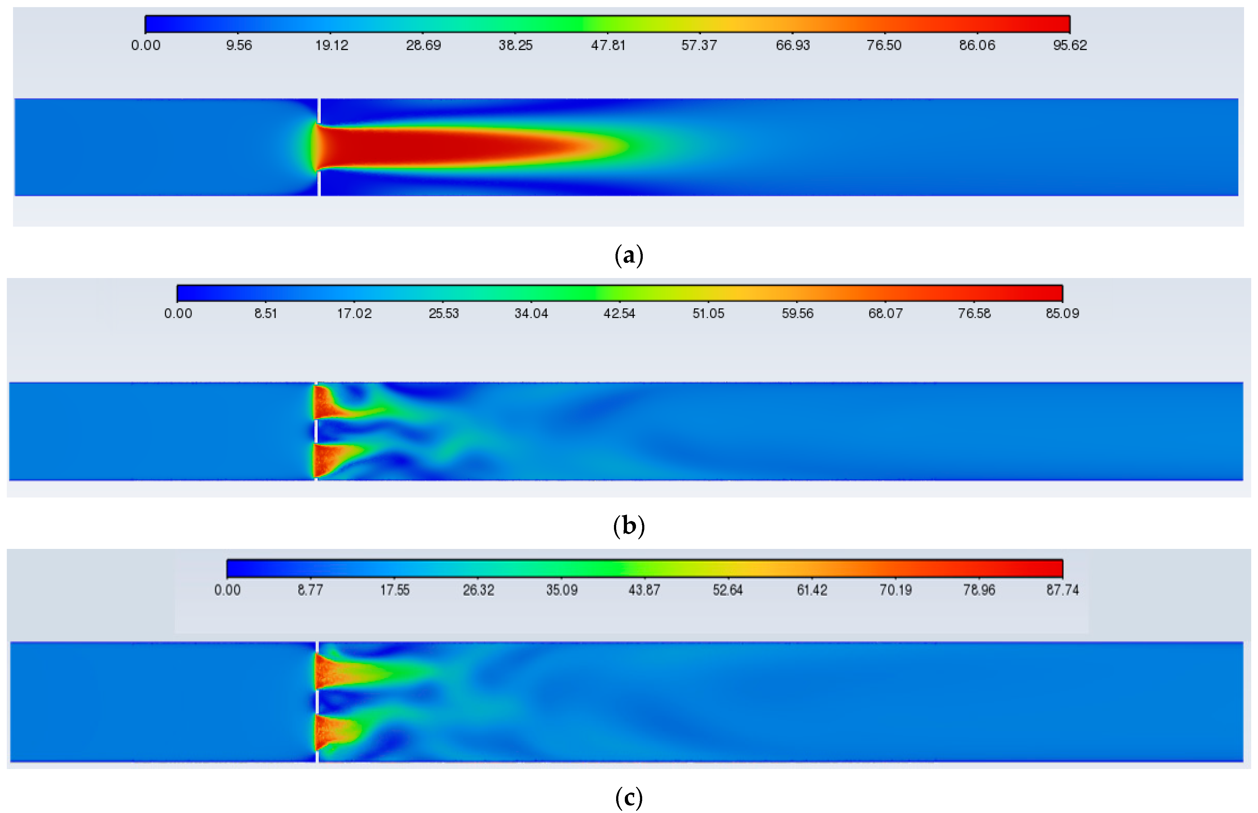
Figure 4 shows the velocity contours for the standard orifice and slotted orifices 1 and 2.

On the basis of the analysis of the above figure, we observed, in the case of special orifices, the separation of the main flow into several smaller ones. The flow became dispersed/separated while the standard orifice generated a compact flow. This distribution of holes in the slotted orifices allowed the resulting streams to interact with each other and the length of the flow stream was shorter compared to a standard orifice. In the case of slotted orifices, it was noted that the flow velocity through such a design solution is lower compared to a standard orifice.

Figure 5 shows the velocity vectors after passing through the different orifice design solutions.

By analyzing the individual figures for the distribution of velocity vectors after passing through the standard orifice and slotted orifices 1 and 2, it could be seen that a zone of turbulence appeared after passing through the orifice. However, in the case of an orifice with a single, centrally located circular hole behind the orifice, it led to the formation of more intense vortices compared to slotted orifices 1 and 2. The sudden narrowing of the flow causes the jet to break off on the outflow side in the case of a classic orifice, creating a clear recirculation zone behind the obstruction. As a result of the radial arrangement of the orifices in the slotted orifices, the recirculation effect behind the orifice was significantly reduced, thus leading to smaller flow disturbances. In the case of the slotted orifices, the recirculation zone occurred directly behind the orifice.

Figure 6 shows the pressure and velocity distributions in the pipeline axis along the entrire length of the flow area.

The centerline velocity and pressure distribution figures along the pipe show the velocity and pressure variations throughout the solution area. The area behind the orifice is the most important zone in the computational domain, because here there is a large velocity gradient and rotational flows occur. It could be seen that the axial velocity of the flow passing through each orifice increased and immediately reached a maximum at one point. For a standard orifice, the maximum value of the flow passing through was about 97 m/s. For slotted orifices, the maximum velocity reached by the flowing gas was much lower compared to the standard orifice and was about 40 m/s. The point of maximum velocity for all orifice design solutions studied was at the same time the point of minimum pressure. Then the velocity began to decrease and at a certain distance reached a velocity equal to the inlet velocity. For slotted orifices, the velocity reached the value of the inlet velocity much faster than for standard orifices. According to the principle of conservation of energy, at the same time as the velocity increases, the pressure decreases and reaches a minimum value at the point of maximum velocity. The pressure then begins to rise, but no longer reaches the initial value. The resulting difference between the inlet pressure and that which occurs at a certain distance behind the orifice is related to energy losses, which are caused by the formation of vortices behind the orifice. In all special orifice models, the pressure drop was about 30–35% less than that of a standard orifice, so the energy savings are greater, and in this respect these models are more suitable compared to a standard orifice. Analyzing the figure further, it could be seen that pressure recovery was much faster with slotted orifices than with standard orifices.

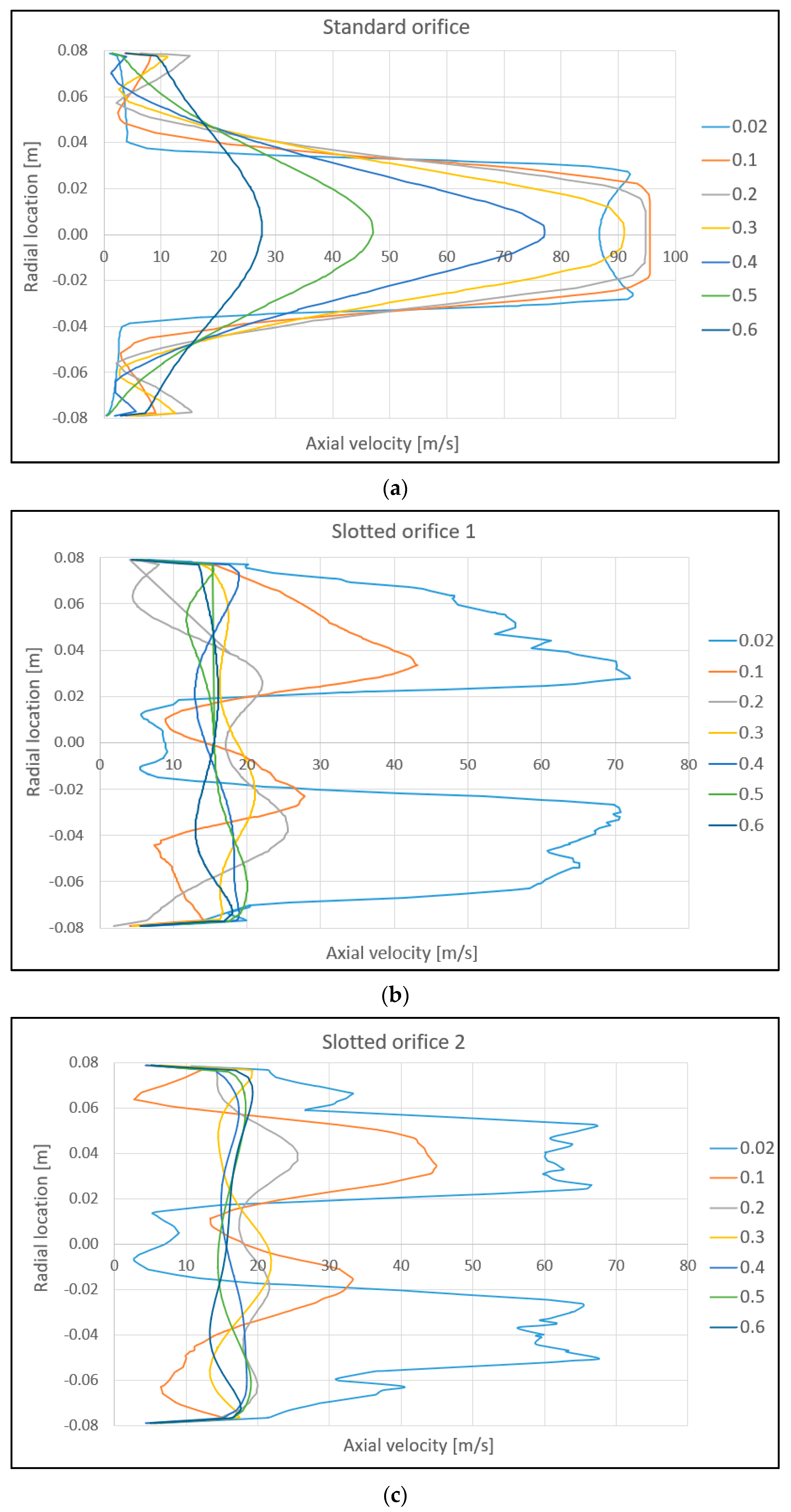
Figure 7 shows the test results for the velocity profiles at different distances behind the standard orifice, as well as slotted orifice 1 and slotted orifice 2. The velocity profiles in each case were determined at the same locations behind the orifice so that it was possible to compare how quickly the velocity profile stabilized after passing each orifice design solution. Transverse velocity profiles were determined at 7 distances behind the orifice, respectively: 2, 10, 20, 30, 40, 50 and 60 cm.

The x-axis shows the velocity values that the fluid flow obtained after passing through the tested orifice. The values on the y-axis indicate the radial location in the pipeline. The individual lines labeled 0.02, 0.1, 0.2, 0.3, 0.4, 0.5, 0.6 indicate the distances behind the orifice, respectively: 2, 10, 20, 30, 40, 50, 60 cm. Analyzing the results obtained for the velocity profile behind the orifice, it could be seen that the velocity at the center of the flow and the velocity gradient on the stream walls in the sections near the orifice were maximum. The maximum stream velocity could be observed for a standard orifice and was about 95 m/s and this maximum velocity occurred at a distance of about 10–20 cm behind the orifice, then the stream velocity decreased, and at a distance of about 60 cm, the stream velocity was about 27 m/s and further stabilized. In contrast, for slotted orifices, the maximum velocity was about 30% lower compared to the flow velocity through a standard orifice. The maximum velocity with slotted orifices occurred immediately behind the orifice and was about 70 and 67 m/s for slotted orifice 1 and slotted orifice 2, respectively. Moving away from the orifices, these magnitudes decreased and at a distance of 20 cm behind the orifice, the flow reached a velocity of about 19 m/s for slotted orifice 1, and an average velocity of about 18 m/s for slotted orifice 2 occurred at a distance of about 30 cm behind the orifice. From the graphs shown above, it can be seen that the jet velocity stabilized at a much shorter distance behind the orifice than for the standard orifice. For slotted orifices, the velocity profile began to stabilize much faster, as the jet began to stabilize at a distance of 20–30 cm.

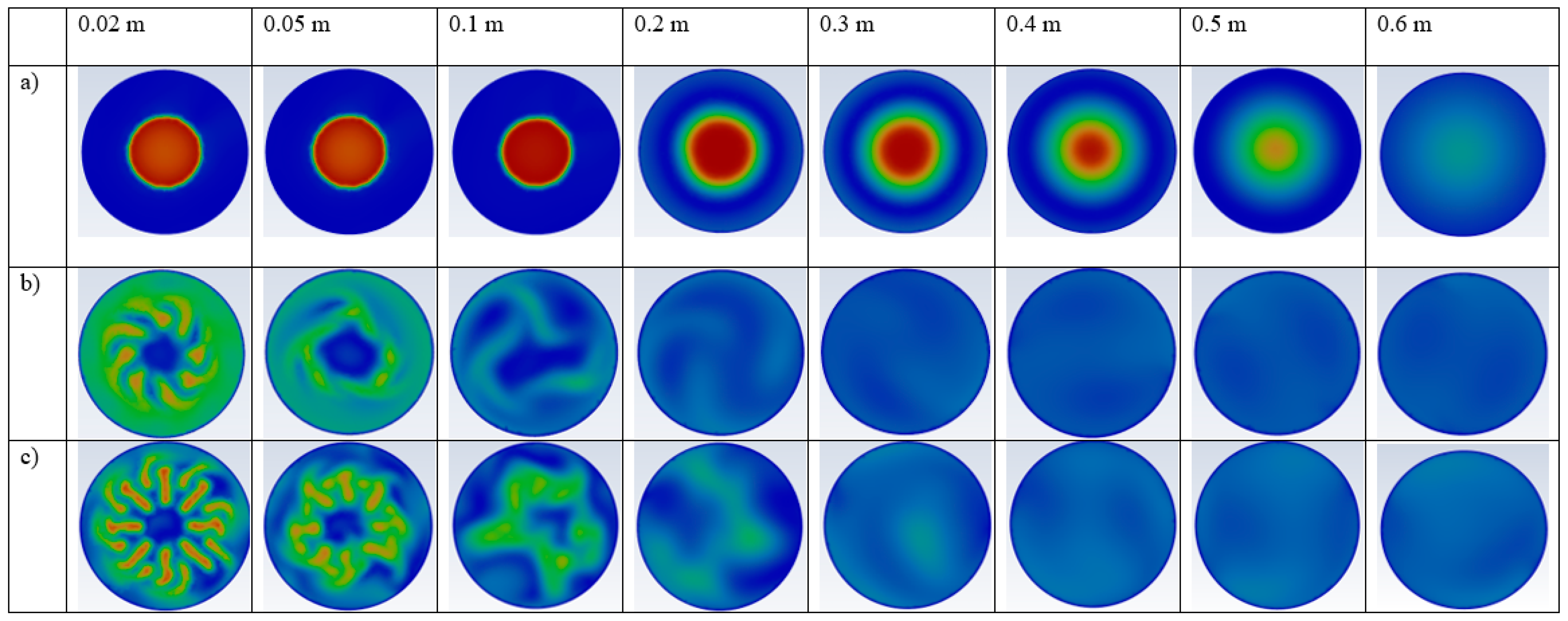
As a supplement to Figure 8, the velocity contours in different planes at specific distances behind the standard orifice, slotted orifice 1 and slotted orifice 2 are shown below.

A comparison of the cross-sections of the flow at eight different distances behind the tested orifice, i.e., 2, 5, 10, 20, 30, 40, 50 and 60 cm is presented in Figure 8. All structural solutions of the orifice were subjected to this analysis. On the basis of the analysis of these graphs, we can see that in the case of a standard orifice, the flow took the form of a compact flux directly behind the orifice, up to a distance of about 30 cm behind the orifice. On the other hand, there was a stagnation zone near the walls of the pipeline. Subsequently, the stream began to occupy the entire cross-section of the pipeline, reaching full stabilization at a distance of 60 cm behind the orifice. In the case of slotted orifices, the slot stagnation effect was eliminated as a result of using slots that were arranged concentrically. The flow through the slotted orifice occupied the entire space of the pipeline directly behind the tested slotted orifice. When we compared both slotted orifice design solutions, we noted that in the case of the first of the solutions, the stream reached stabilization at a distance between 10 and 20 cm behind the orifice, while in the case of slotted orifice 2, the stream stabilized at a distance of about 20 to 30 cm behind the orifice. The vena contracta zone forms an important design aspect of orifices as it affects the performance and effectiveness of the entire flow system. Understanding and taking into account the vena contracta area enables the optimal design of flow systems combined with the minimization of energy losses. Therefore, in the context of the occurrence of the vena contracta zone, it was important to find a design solution for the measuring orifice that will be able to significantly reduce the occurrence of this zone.

In the following, the results of the obtained values of the kinetic energy of turbulence and the rate of dissipation of this energy at seven different distances behind the orifice are presented. The value of the kinetic energy of turbulence is shown from the orifice to the fully developed turbulent flow behind the orifice. Turbulence kinetic energy is the average kinetic energy per unit mass of fluid with respect to turbulent flow structures. Turbulent kinetic energy is created by shear force and the agitation of motion. Shear transforms the average kinetic energy into turbulence, but also simultaneously excites and creates it as a result of work against frictional forces. Physically, turbulent kinetic energy is characterized by the standard deviation of velocity fluctuations. In contrast, the dispersion velocity of turbulent kinetic energy is the dissipation velocity of turbulent kinetic energy.

Figure 9 and Figure 10 show the results of these tests for the orifices tested.

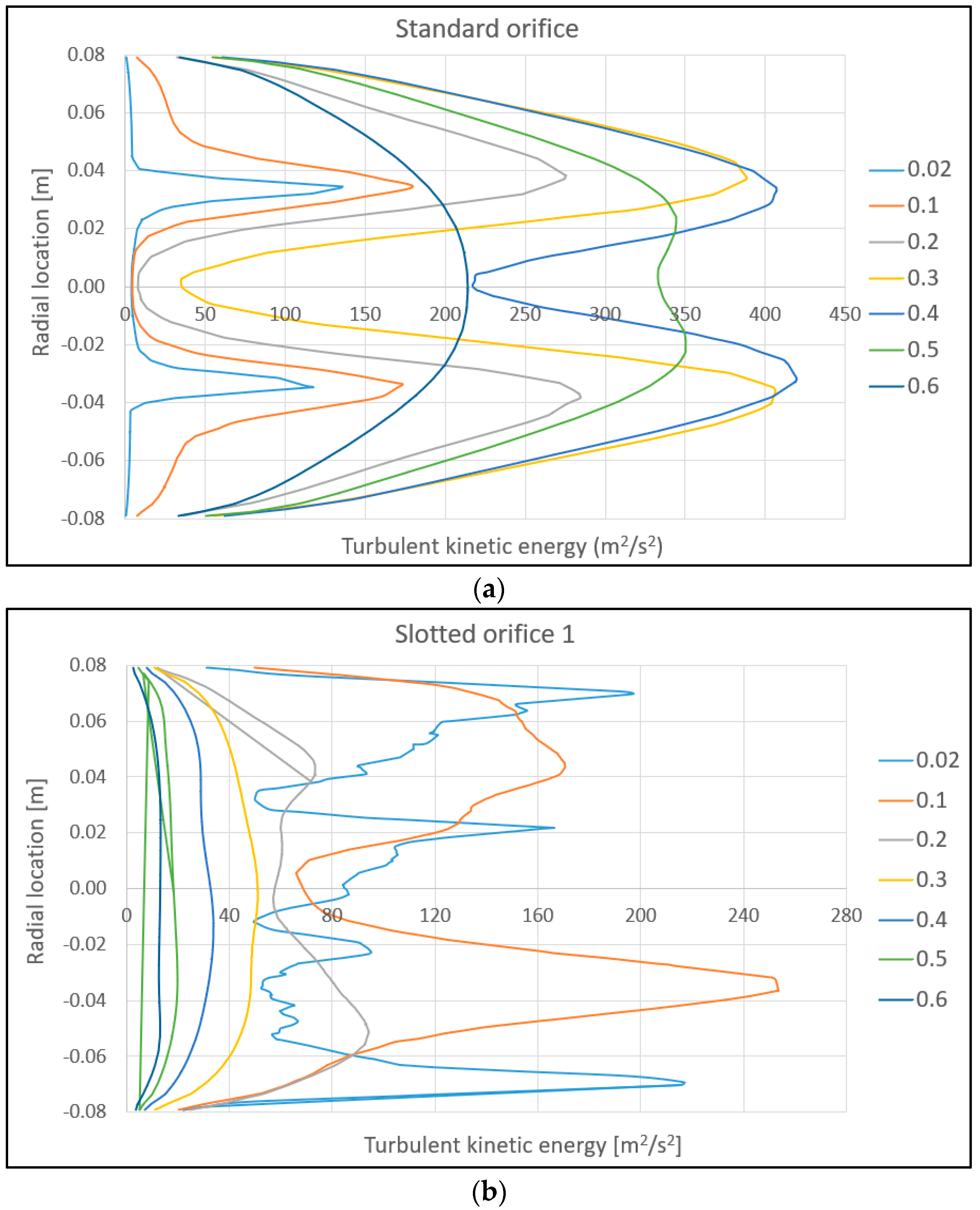
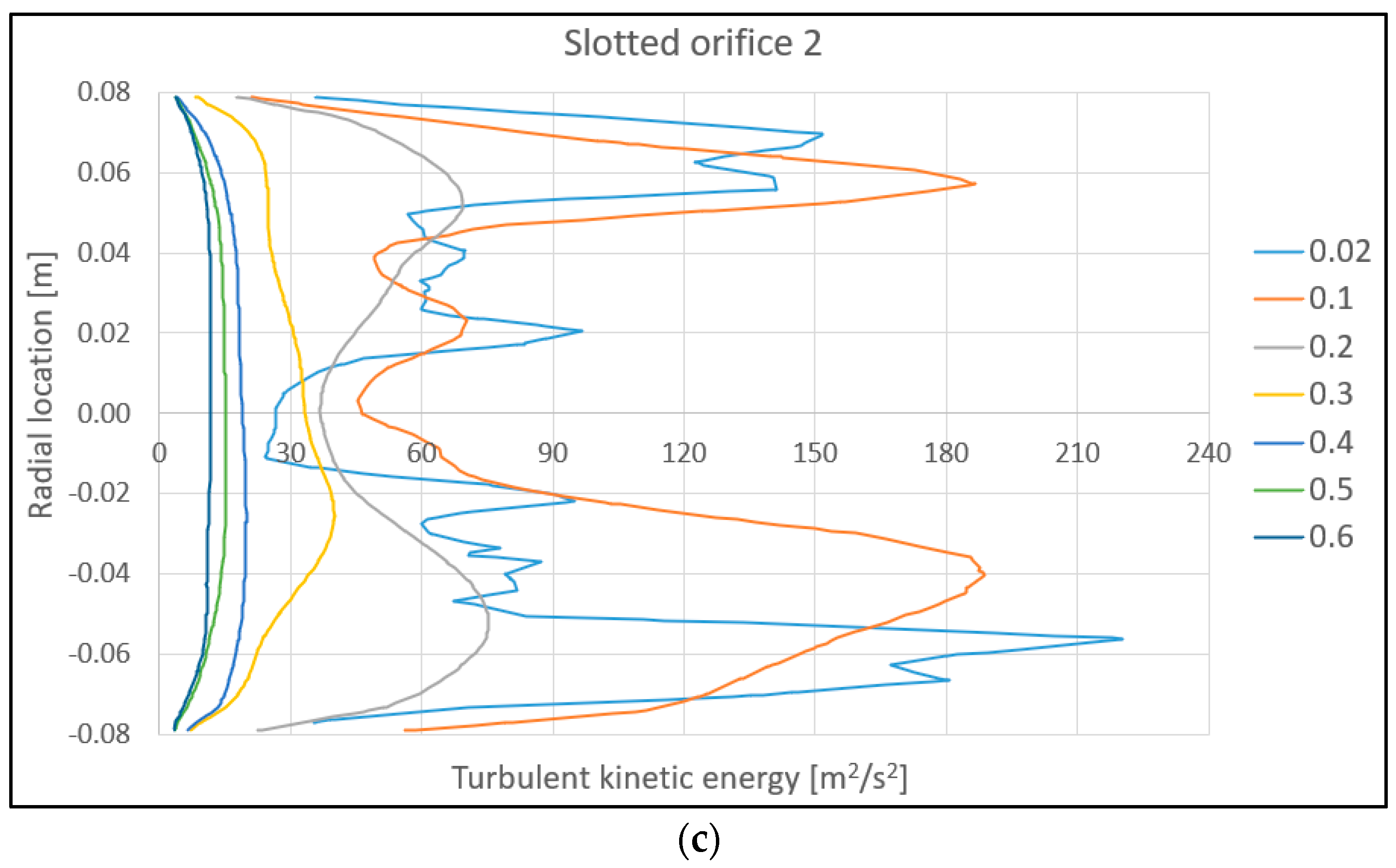
The graphs presented in Figure 9 and Figure 10 show the development of the turbulence kinetic energy and turbulence energy dispersion coefficient for all the orifices tested. The graphs show the radial profiles of the characteristics of the kinetic energy of turbulence and the radial profiles of the turbulence energy dispersion coefficient in seven different planes behind the tested orifices, starting from the surface directly behind the orifice. The lines, which are labeled 0.02, 0.1, 0.2, 0.3, 0.4, 0.5, 0.6, indicate the distances behind the tested orifice, respectively: 2, 10, 20, 30, 40, 50, 60 cm.

By analyzing the above graphs, it could be seen that the turbulence kinetic energy was highest for the standard orifice, where the maximum value of turbulence kinetic energy was about 420 m²/s². This maximum value was observed at a distance of about 40 cm behind the orifice. In the case of the standard orifice, such a distribution of kinetic energy values in the different planes was due to the presence of a large velocity gradient at the periphery of the stream. The kinetic energy of turbulence reached maximum values at the periphery of the stream of flowing fluid, while in the center of the stream, the kinetic energy in individual sections reached minimum values, which was due to the conversion of pressure to velocity in the throat of the flow.

Analyzing the graphs for the slotted orifices, it could be seen that at the outlet of each slot, the magnitude of turbulence kinetic energy reached maximum values and the dispersion of velocity turbulence energy were maximum, and for slotted orifice 1 and slotted orifice 2 were 250 and 220 m²/s², respectively. These maximum values of turbulence kinetic energy were reached at the distance immediately behind the orifice, that is, at a distance of 2 to 10 cm. After that, these values began to decrease.

It was also observed that moving away from the slots, the average turbulence energy dissipation rate for slotted orifices 1 and 2 decreased comparably. In the case of slotted orifices, energy dissipation began directly and at a slight distance behind the orifice. At the same time, the value of the kinetic energy dispersion coefficient was higher for slotted orifices compared to the standard orifice. This was due to the increase in the number of flow holes in the slotted orifices. The obtained results on turbulence kinetic energy and energy dispersion led us to the conclusion that one of the most important differences between the studied orifices was the length of the developing turbulent region behind the hole, which was significantly shorter for slotted orifices.

Table 2. Comparison of differential pressures and discharge coefficients for standard and two phase flow orifices.

Orifice	Differential Pressure Δp [Pa]	Discharge Coefficient C
Standard	5390	0.619
Slotted 1	3841	0.733
Slotted 2	3577	0.759

below shows the test results for comparing the resulting pressure differences and discharge coefficients for standard orifice and slotted orifices.

Analyzing the table described above, the slotted orifices, compared to an orifice with a single, circular, centrally located hole, resulted in a smaller differential pressure at the orifice. Slotted orifice 1 resulted in a pressure difference of about 28% less, while slotted orifice 2 resulted in a pressure difference of about 33% less compared to the differential pressure for a standard orifice. The values of the flow coefficient for slotted orifice 1 and slotted orifice 2 were higher compared to the standard orifice and higher than the value of the flow coefficient for the standard orifice by 15 and 18%, respectively.

4. Conclusions

In this paper, a numerical analysis of fluid flow through various design solutions of a differential pressure flowmeter was carried out. This analysis included a standard orifice and two slotted orifices, designated as slotted orifice 1 and slotted orifice 2.

The numerical calculations carried out in the paper were intended to check, among other things, the behavior of the fluid flow through the measuring orifice. Furthermore, the analysis involved the behavior of the air flowing through different geometrical orifice solutions. The simulation studies made it possible to analyze velocity profiles, turbulence kinetic energy profiles and turbulence energy dispersion profiles, at different distances behind the orifice. In addition, the pressure distribution and velocity distribution along the pipeline axis were also analyzed. The means by which the flowing fluid is shaped by a given geometrical solution was also checked. The distribution of velocity vectors around the orifice was also checked. From the obtained results of the numerical tests, the conclusions included an observation that slotted orifices under single-phase fluid flow conditions lead to a smaller pressure difference compared to the standard orifice. Another difference between the tested orifices was that the slotted orifices led to a smaller permanent pressure loss compared to the classical solution. Slotted orifices were also characterized by a faster pressure recovery. This is mainly due to the fact that the resulting large vortices generated during throughflow in the standard orifice are the cause of the creation of greater permanent pressure loss and slower pressure recovery. The resulting vortices behind the slotted orifices are generated in close proximity behind the orifice and are smaller compared to the classic solution. By replacing the circular hole with slots, slotted orifices do not provide as much resistance to the flowing fluid; hence, a lower value of the differential pressure is created at the orifice. The distribution of slots in the slotted orifices allows the length of the hydraulic stabilization section of the jet to be reduced. This is due to the fact that the flow is separated into several smaller streams, and thus a large recirculation zone is not formed behind the orifice. The large recirculation zone formed behind the standard orifice is the main cause of energy losses. Based on the simulation results obtained, it can also be concluded that slotted orifices lead to a faster homogenization of the jet than in the case of a standard orifice. One disadvantage of the standard orifice is that long straight sections are required to perform correct measurements. The use of slotted orifices allows the required straight pipe sections behind the orifice to be significantly reduced. However, the use of slotted orifices can assist in eliminating the phenomenon of cavitation in the hydraulic system in which the orifice is installed. This is due to the radial arrangement of the slots, as a result of which, the flow occupies the entire volume of the pipeline. However, it is reasonable to conduct research on the influence of the orifice shape on the phenomenon of cavitation.