Reasons for the Recent Onshore Wind Capacity Factor Increase

Abstract

Increasing wind capacity and capacity factors (CF) are essential for achieving the goals set by the Paris Climate Agreement. From 2010–2012 to 2018–2020, the 3-year mean CF of the global onshore wind turbine fleet rose from 0.22 to 0.25. Wind turbine siting, wind turbine technology, hub height, and curtailed wind energy are well-known CF drivers. However, the extent of these drivers for CF is unknown. Thus, the goal is to quantify the shares of the four drivers in CF development in Germany as a case. Newly developed national power curves from high-resolution wind speed models and hourly energy market data are the basis for the study. We created four scenarios, each with one driver kept constant at the 2010–2012 level, in order to quantify the share of a driver for CF change between 2010–2012 and 2019–2021. The results indicated that rising hub heights increased CF by 10.4%. Improved wind turbine technology caused 7.3% higher CF. However, the absolute CF increase amounted to only 11.9%. It is because less favorable wind turbine sites and curtailment in the later period moderated the CF increase by 2.1% and 3.6%, respectively. The drivers are mainly responsible for perennial CF development. In contrast, variations in wind resource availability drive the enormous CF inter-annual variability. No multi-year wind resource change was detected.

1. Introduction

Replacing conventional energies with renewables is urgently needed for climate change mitigation. One step toward a decarbonized energy system is the globally installed onshore wind capacity (IC) of 769 GW [1]. However, to meet the 1.5 °C target, the worldwide onshore installed capacity must increase to more than 5000 GW in 2050 [2]. The wind turbine fleet is unevenly distributed around the world since three countries, China (IC = 303 GW), the USA (IC = 133 GW), and Germany (IC = 56 GW), comprise almost two-thirds of the globally installed capacity.

Another requirement to achieve the 1.5 °C target is the rising wind turbine capacity factor (CF) derived from wind turbine power output and rated power (P_r). Recently, the 3-year mean capacity factor of the global onshore wind turbine fleet rose from 0.22 in 2010–2012 to 0.25 in 2018–2020 [1]. National capacity factor values vary, as shown by the capacity factor values in 2020, being 0.19 in China and 0.33 in the USA. The capacity factor is also subject to annual fluctuations. In 2010–2021, Germany’s capacity factor ranged from 0.163 in 2010 to 0.217 in 2020 (Figure 1a). An analysis of the capacity factor values over a 3- and 5-year moving time window (Figure 1b,c) reveals a positive linear trend. A relevant inter-annual variability is also apparent. Potential drivers for the spatiotemporal capacity factor variability are (1) wind turbine siting, (2) hub height, (3) wind turbine technology, and (4) curtailed wind energy. Wind turbine site suitability depends on the available wind resource, geographical restrictions, and the socio-economic potential [3,4,5,6].

The capacity factor is affected by spatiotemporally diverse wind resources and turbine characteristics. Wind speed (U) predominantly determines wind resources. It has an enormous spatiotemporal variability. Spatially, wind speed differs depending on the latitude, longitude, land–sea distribution, orography, and land use [7]. Sub-hourly, hourly, daily, seasonal, and annual wind speed variations are part of the temporal variability [8]. Wind speed also has long-term variability in the range of decades, caused by the natural, internal decadal ocean/atmosphere oscillations of the climate system [9]. One example is the global terrestrial stilling from 1980 to 2010 and its reversal ever since. Likewise, anthropogenic climate change is altering global circulation systems and wind speed. A weakening of the air temperature gradient between the north pole and mid-latitudes could decrease future wind speeds [10] in many areas of the northern hemisphere with high installed capacity [11]. Another influencing factor for wind speed is the wake effect in wind farms, which lowers wind speed at individual wind turbine sites. However, the spatial extent to which existing wind turbines reduce the wind resource is difficult to quantify. Some studies indicate that wind turbine-induced wind speed decreases due to the extraction of kinetic energy could even cover whole countries or the globe [12]. Recently, Li et al. [13] assumed that although onshore wind farms reduce local wind speeds, their influence is insufficient to overcome oceanic/atmosphere oscillations, and at their currently installed capacity, they do not affect the global wind speed distribution.

Wind speed increases logarithmically with increasing height above ground [14,15]. Thus, the hub height (hhub) of wind turbines is relevant for the capacity factor [16]. A general trend toward higher hub heights in recent years exists [17]. Increasing the hub height from 120 m to 140 m leads to higher global wind potential by about 12% [18]. Regional case studies also indicate increasing wind turbine power output as indicated for China, where the same hub height increase led to approximately 7% higher energy yields [19]. Thus, previously undeveloped low-wind resource regions become more prospective for wind turbines [20].

The increase in hub height is not the only trend of modern wind turbines. Many turbine features have improved recently, leading to rising capacity factor values [21]. Higher rated power (P_r) and larger rotor diameters (RD) characterize the development of the global wind turbine fleet [22]. One parameter quantifying the better wind resource exploitation of modern wind turbines is the specific rating, which is the ratio of rated power to rotor swept area [23]. New wind turbine installations are also advantageous over the old because wind turbine performance declines smoothly with age [24]. The reasons for decreasing power outputs are deteriorating component reliability, aerodynamic and mechanical efficiency losses, and more downtime. The wind turbine power curve considers all components influencing wind turbine performance, as it defines the relationship between the wind turbine power output or capacity factor, and wind speed [25,26]. The main features of a power curve are the cut-in speed, rated speed, and cut-out speed.

Wind energy curtailment considerably reduces the capacity factor. One major disadvantage of wind energy is its non-dispatchable nature [27,28]. The increasing share of variable renewable energy in the power grid sometimes requires wind power curtailment [29,30]. Curtailment is defined as the reduction in the output of a generator from what it could otherwise produce given available resources [31]. One reason for curtailment is congestion in the transmission system [32]. Interconnection and battery deployment enable the reduction in curtailment [33]. In countries with high installed capacities, such as China [34] and Germany [35], wind energy curtailment leads to relevant capacity factor reduction.

The theoretical and qualitative influences of the wind turbine siting, hub height, technology, and curtailed wind energy on the capacity factor are well described and understood. For individual wind turbine sites, it is often also possible to quantify the influence of capacity factor drivers. In contrast, there is a lack of quantitative estimates considering the combination of the above capacity factor drivers for national wind turbine fleets. Therefore, it is unknown how much hub height increases and improved technology are responsible for the capacity factor increase in many countries in recent years. It is also unclear how much decreasing wind resources at wind turbine sites possibly prevented even higher capacity factor values.

Thus, the goal of this study was to quantify the shares of wind turbine (1) siting, (2) technology, (3) hub height, and (4) curtailment in capacity factor development. We structured this research as a case study of Germany’s onshore wind turbine fleet, since the installed capacity in that country is very high, and increased by 109% from 2010 to 2021. In addition, Germany has a high onshore wind turbine density that allows us to test the hypothesis that the 2010–2021 capacity factor increase was capped by decreasing wind speed due to wind energy expansion.

2. Materials and Methods

The workflow to quantify the shares of the drivers in CF development (Figure 2) comprise the following main steps: (1) obtaining wind turbine fleet data, including site coordinates and hub heights from the German power plant platform Markstammdatenregister [36]; (2) obtaining the 6-hourly wind speeds at wind turbine sites from a German wind atlas [37]; (3) quantile mapping with reanalysis wind speed data [38] to develop hourly wind speed time series; (4) gaining national wind energy yield data from the Energy-Charts platform [39]; (5) developing national power curves from wind speed and energy yield data; (6) obtaining curtailed wind energy yield; and (7) quantifying the shares of the drivers in CF development.

2.1. Wind Turbine Fleet Data

The platform Marktstammdatenregister (MaStR) [36] hosted by the German Federal Network Agency contains information regarding the operating and planned electricity and gas generation plants in Germany. We extracted the data for all wind turbine sites operating at the end of 2021. The entries for the wind turbines included information on the date of commissioning, hhub, P_r, RD, turbine type, and explicit coordinates. Based on the year of commissioning, we created annual wind turbine fleets for 2010–2021.

2.2. Wind Speed Data

We used three different wind speed datasets in this study. The first dataset is the Wind Speed Complementarity model (WiCoMo) [37], a high-spatiotemporal resolution model developed for adjusting wind turbine site selection to residual load. It contains the Kappa distribution parameters (α, k, μ, o) at a 25 m × 25 m spatial resolution grid covering Germany. The grid cell-related Kappa quantile functions (U_WiCoMo (F)) were calculated by [40,41,42]:

$$U_{WiCoMo}\left(F\right)=\mu +\frac{\alpha }{k}\left[1-{\left(\frac{1-F^o}{o}\right)}^k\right]$$

(1)

The second dataset is the model Uncertainties in Ensembles of Regional Re-Analyses (U_ERRA) [43]. U_ERRA has a spatial resolution of 11 km × 11 km, and is 6-hourly available from 1961–2019. It provides the regional scale wind speed for parameterization of WiCoMo. In this study, we used the U_ERRA variables wind speed in 10 m (U_UERRA,10) and wind speed in 100 m (U_UERRA,100).

The third dataset is the fifth-generation ECMWF atmospheric reanalysis of the global climate (ERA5) model [38]. The spatial resolution is 0.25° × 0.25°. The ERA5 variables are available hourly from 1959 onwards. The relevant variables for the current study are the wind vector components at 10 m (u_ERA5,10, v_ERA5,10) and 100 m (u_ERA5,100, v_ERA5,100). The wind vector components were used to calculate the hourly wind speed at 10 m (U_ERA5,10) and 100 m (U_ERA5,100) with the following:

$$U_{ERA5,10}=\sqrt{u_{ERA5,10}{}^2+v_{ERA5,10}{}^2}$$

(2)

and the following:

$$U_{ERA5,100}=\sqrt{u_{ERA5,100}{}^2+v_{ERA5,100}{}^2}$$

(3)

The goal was to generate hourly wind speeds on the 25 m × 25 m WiCoMo grid in 2010–2021 for heights of 10 m (U_10,HR), 90 m (U_90,HR), and the wind turbine hub (U_hhub,HR) based on the presented variables from the three wind speed datasets.

Building the U_10,HR model required several intermediate steps. Firstly, the coarsely resolved U_ERA5,10 and U_ERA5,100 time series were converted to the higher resolution U_ERRA grid by quantile mapping [44,45], resulting in U_QM,10 and U_QM,100 time series. Next, the U_QM,10 time series were further quantile-mapped to the WiCoMo grid, yielding U_10,HR.

The extrapolation of the U_10,HR to 90 m and hhub also required several steps, following the approach presented in [37]. First, hypothetical wind speed at 2000 m (U_QM,2000) at the UERRA grid was calculated by estimating the power law exponents (PLE_QM):

$$PL{E}_{QM}=\frac{ln\left(\frac{U_{QM,100}}{U_{QM,10}}\right)}{ln\left(\frac{100 \mathrm{m}}{10 \mathrm{m}}\right)}$$

(4)

and applying the power law:

$$U_{QM,2000}=U_{QM,10}{\left(\frac{2000 \mathrm{m}}{10 \mathrm{m}}\right)}^{PL{E}_{QM}}$$

(5)

Based on the U_QM,2000 and U_10,HR, the high-resolution PLE time series were generated by the following:

$$PLE=\frac{ln\left(\frac{U_{QM,2000}}{U_{QM,10}}\right)}{ln\left(\frac{2000 \mathrm{m}}{10 \mathrm{m}}\right)}$$

(6)

Using the power law, the U_90,HR was calculated as follows:

$$U_{90,HR}=U_{10,HR}{\left(\frac{90 \mathrm{m}}{10 \mathrm{m}}\right)}^{PLE}$$

(7)

The U_90,HR time series were extracted at all grid cells with a wind turbine. The mean of the U_90,HR values was used to build the national mean U_90,HR time series (U₉₀). National time series were also created for the U_hhub,HR (U_hhub) data by averaging the U_hhub,HR values, assuming the actual hhub for each wind turbine location.

2.3. Energy Market Data

The platform Energy-Charts from Fraunhofer ISE [39] provides many energy market data. We used the national hourly onshore wind energy generation (OWE) from 2010–2021. The variable OWE is an estimation by the transmission system operators based on reference wind turbines. The annual installed IC in 2010–2021 was also available from Energy-Charts.

A monitoring report from Germany’s Federal Network Agency and the German Federal Cartel Office contains outage work caused by feed-in management measures for many energy sources [46]. We used the report as the data source for the annually curtailed wind energy (CUE) in 2011–2020.

2.4. Development of National Power Curves

The development of national power curves started with calculating hourly CF values for each year with the following:

$$CF=\frac{OWE}{IC\times 8760 \mathrm{hr}}$$

(8)

Two variants of power curves with the mean U_hhub and U₉₀ including all installed wind turbines were built. The U_hhub and U₉₀ values were plotted against the CF for each year. Then, smoothing splines [47] with a parameter of 0.5 were fitted, yielding the national power curves. The goodness-of-fit was evaluated using the coefficient of determination (R²).

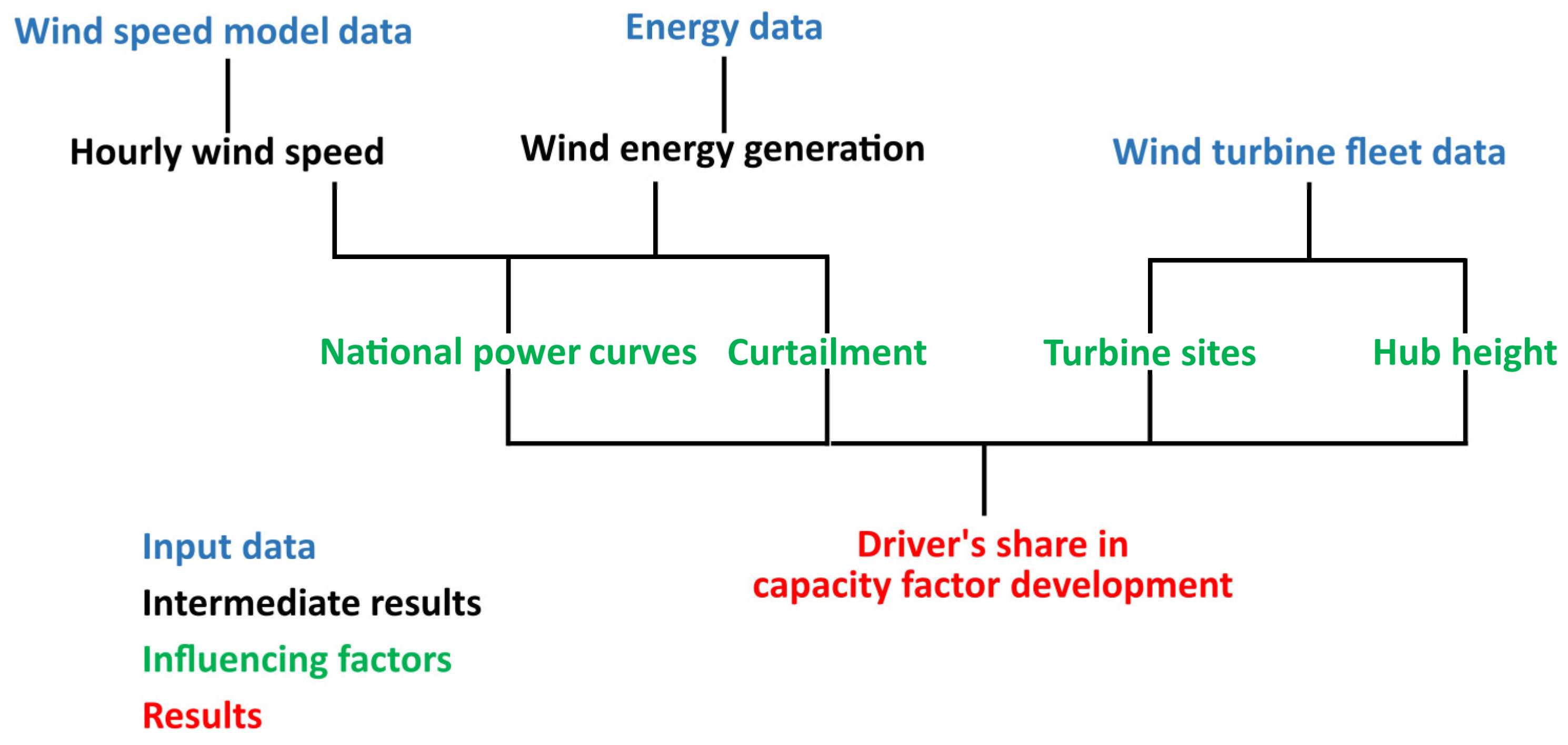
2.5. Quantification of the Shares of the Drivers

We calculated the difference between the CF in 2019–2021 and 2010–2012 (ΔCF) as a function of wind speed classes for U₉₀ and U_hhub. When ΔCF > 0, the CF for a given wind speed class has increased between the first and second period. When ΔCF < 0, the CF for a given wind speed class has decreased between the first and second period. Thus, ΔCF was used to analyze for which U classes the increase in the CF is mainly due.

The ΔCF curves provide another option. Comparing the course of ΔCF by U_hhub and U₉₀ enables the effect of the h_hub increase on the annual changes of the power curves to be quantified. The higher ΔCF for U₉₀ compared to ΔCF for U_hhub, the more the CF increase is due to the rise in hhub.

We developed four scenarios, each with one driver kept constant at the mean 2010–2012 level, in order to quantify the share of a driver for CF change. The other three drivers were kept at the mean 2019–2021 level. The first scenario (S1) assumed the wind turbine sites as they were in 2010. The second scenario (S2) assumed the technology as in 2010–2012. The third scenario (S3) assumed the hub heights as they were in 2010–2012. The fourth scenario (S4) assumed the curtailment as it was in 2010–2012. In addition, one scenario (S19–21) kept all of the conditions as they were in 2019–2021.

The CF values were calculated assuming S1–S4 and S19–21. Different variants of the variables were used to calculate CF values for the scenarios. They are listed in

Table 1. Summary of the investigated scenarios S19–S21, S1, S2, S3, and S4 with height, power curve, curtailment factor, and sites.

Scenario	Description	Height	Power Curve	Curtailment	Sites
S19–21	conditions as in 2019–2021	90 m	2019–2021	no factor	2019–2021
S1	wind turbine sites as in 2010	90 m	2019–2021	no factor	2010
S2	technology as in 2010–2012	90 m	2010–2012	factor (1.038)	2019–2021
S3	hub height as in 2010–2012	hhub	2019–2021	no factor	2019–2021
S4	curtailment as in 2010–2012	90 m	2019–2021	factor (0.964)	2019–2021

. Changes in the mean CUE between 2010–2012 and 2019–2021 were considered using a factor which represents the increasing share of CUE in OWE.

Finally, the difference between the mean CF in 2019–2021 and the scenario-based CF was calculated. The magnitude and direction of ΔCF quantified the influence of (1) wind turbine siting (S1), (2) technical improvement (S2), (3) hub height increase (S3), and (4) curtailment (S4) on CF.

3. Results and Discussion

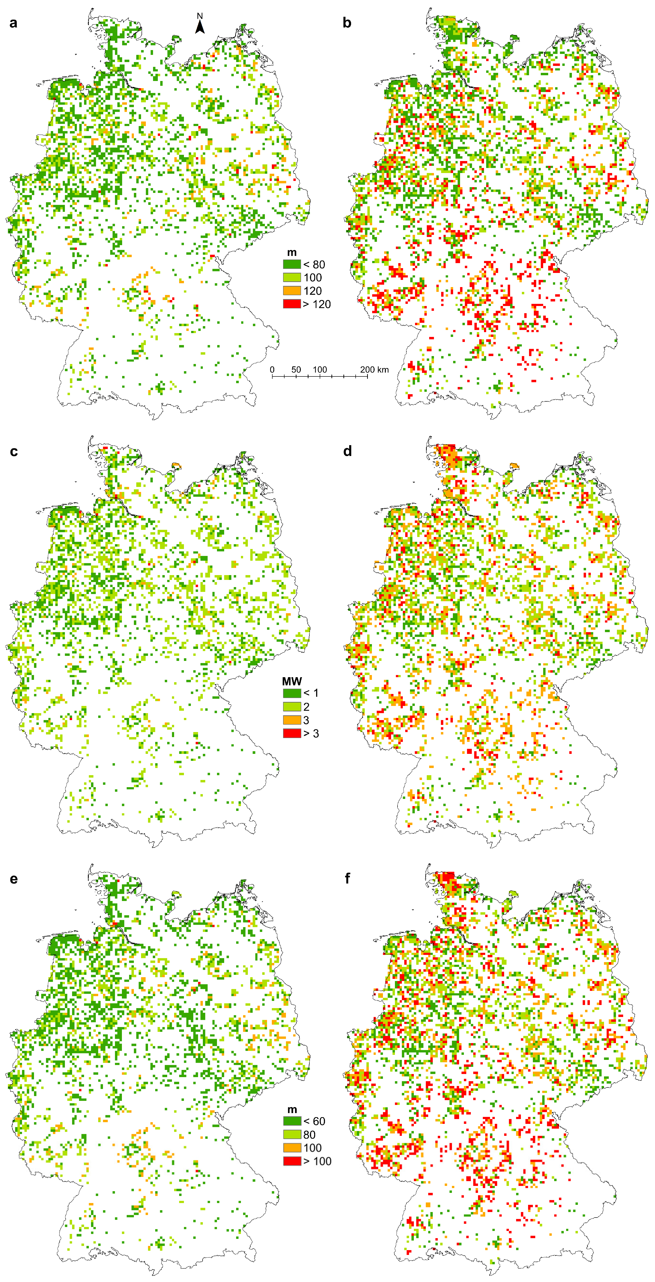
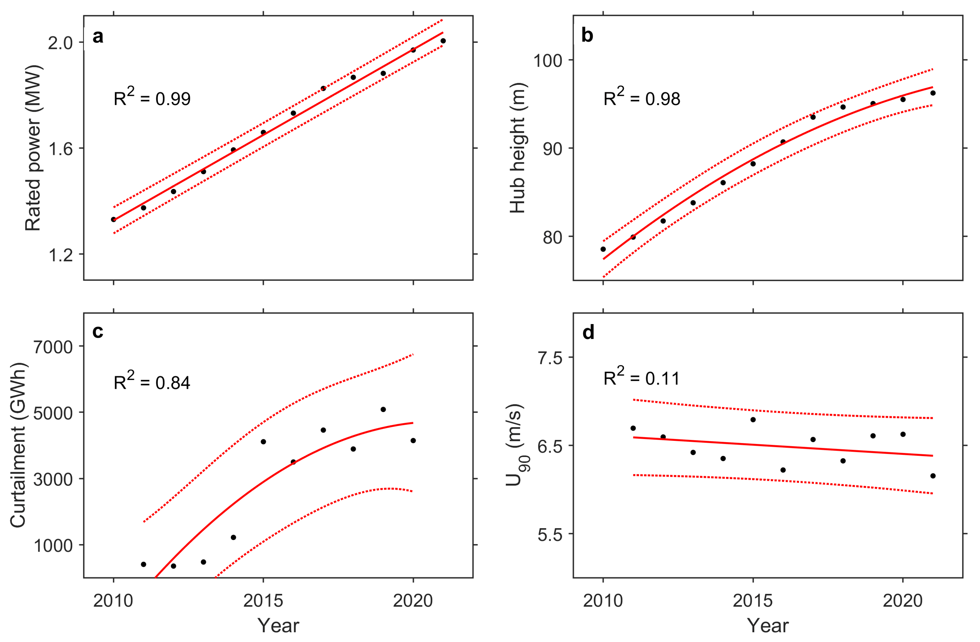
3.1. Development of Technical Features and Wind Resource

Figure 3 compares the spatial distribution of the technical features hhub, P_r, and RD between the 2010 and 2021 wind turbine fleets.

In 2010, the mean hhub in Germany was 78.6 m (Figure 3a). At 19.9% of all of the sites, the hhub was even below 70 m. Many of these wind turbines are in the northwest. One reason is the lower U increase with hhub in this region because of the generally low surface roughness. Nevertheless, there are also sites with a low hhub in other parts of the country. Only 25.9% of all wind turbine sites have hhub > 100 m. They occur throughout the country. The mean hhub increased to 97.4 m in 2021 (Figure 3b). The majority of wind turbines (54.7%) have hhub > 100.0 m. A relevant proportion of sites (17.5%) even have hhub > 140 m. They are mainly in the southern half of the study area, where the pronounced orography requires a higher hhub.

Figure 3c displays the P_r of 2010. The mean of P_r was 1.33 MW, and 69.4% of the wind turbines exceeded 1.00 MW. The proportion of such sites was higher in the northeast and southwest than in many other parts. Many wind turbines with PR > 2.00 MW are limited to the northwest. However, the share of P_r > 2.00 MW wind turbines was low (2.3%). In 2021, the mean P_r increased to 2.00 MW. More than two-thirds of the wind turbines (69.4%) had a P_r > 2.00 MW. There were no distinct hot spot areas of such wind turbines. However, the proportion of P_r > 2.00 MW wind turbines was higher in the south than in the north.

The mean RD in 2010 was 64.8 m (Figure 3e). Only about one-third of all wind turbines (32.3%) had an RD > 80 m. Many of these wind turbines are in the east. Almost no wind turbine (0.04%) had an RD >100 m. Most of these pioneering wind turbines are in the north. In 2021, the mean of RD rose to 81.8 m (Figure 3f). Now, the majority of the wind turbines (53.9%) have an RD > 100 m. In some locations (2.9%), RD exceeds 140 m.

The P_r and hhub increases in the wind turbine fleet are continuous processes that do not occur suddenly. The P_r values increased quasi-linearly between 2010 and 2021 (Figure 4a). This happens because the wind turbine fleet is constantly supplemented with new wind turbines of higher P_r values, and old wind turbines with lower P_r values are being decommissioned [11]. The smallest mean P_r increase was between 2018 (1.87 MW) and 2019 (1.88 MW) because the wind capacity increase in 2019 was substantially less than in previous years.

The hhub values were also higher each year than the previous year (Figure 4b). The reasons for this development correspond to those for the P_r. In contrast to the P_r, the hhub increase has moderated in recent years. Thus, the decrease in newly installed capacity per year has more impact on hhub than on P_r. Accordingly, a second-degree polynomial reproduces the hhub slope better than a first-degree polynomial.

The role of onshore wind curtailment increased as the share of intermittent renewables in the electricity mix increased (Figure 4c). The CUE values rose from 410 GWh in 2011 to 4145 GWh in 2020. The development of CUE has more fluctuations than the wind turbine properties P_r and hhub because the CUE depends on many more factors, including energy market properties [31]. The year with an abrupt CUE increase was 2015. In 2014, CUE = 1222 GWh, but in 2015, CUE = 4111 GWh.

The wind turbine fleets from 2010 to 2021 operated under different wind resource availability (Figure 4d). The U₉₀ values had a high degree of inter-annual variability. In the Appendix A Figure A1 presents CF for each year between 2010 and 2021. The inter-annual variability in U₉₀ was much more significant than the slight downward tendency. There are two possible rationales for the U₉₀ decline. The first reason is that the wind speed in the study area is generally decreasing [12]. The second reason is that the siting quality of new wind turbines is decreasing. As will be pointed out in the following sections, the decrease in siting quality caused the decreasing U₉₀ values.

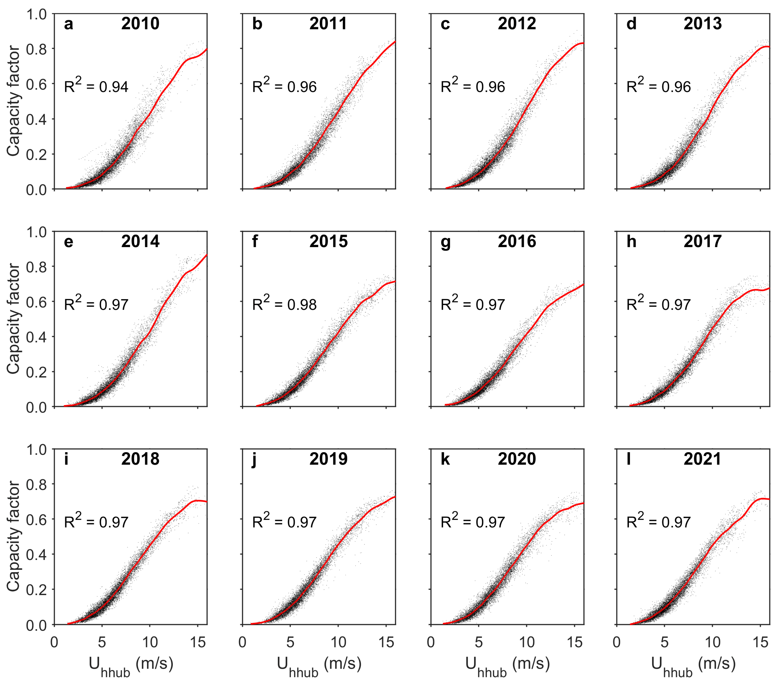
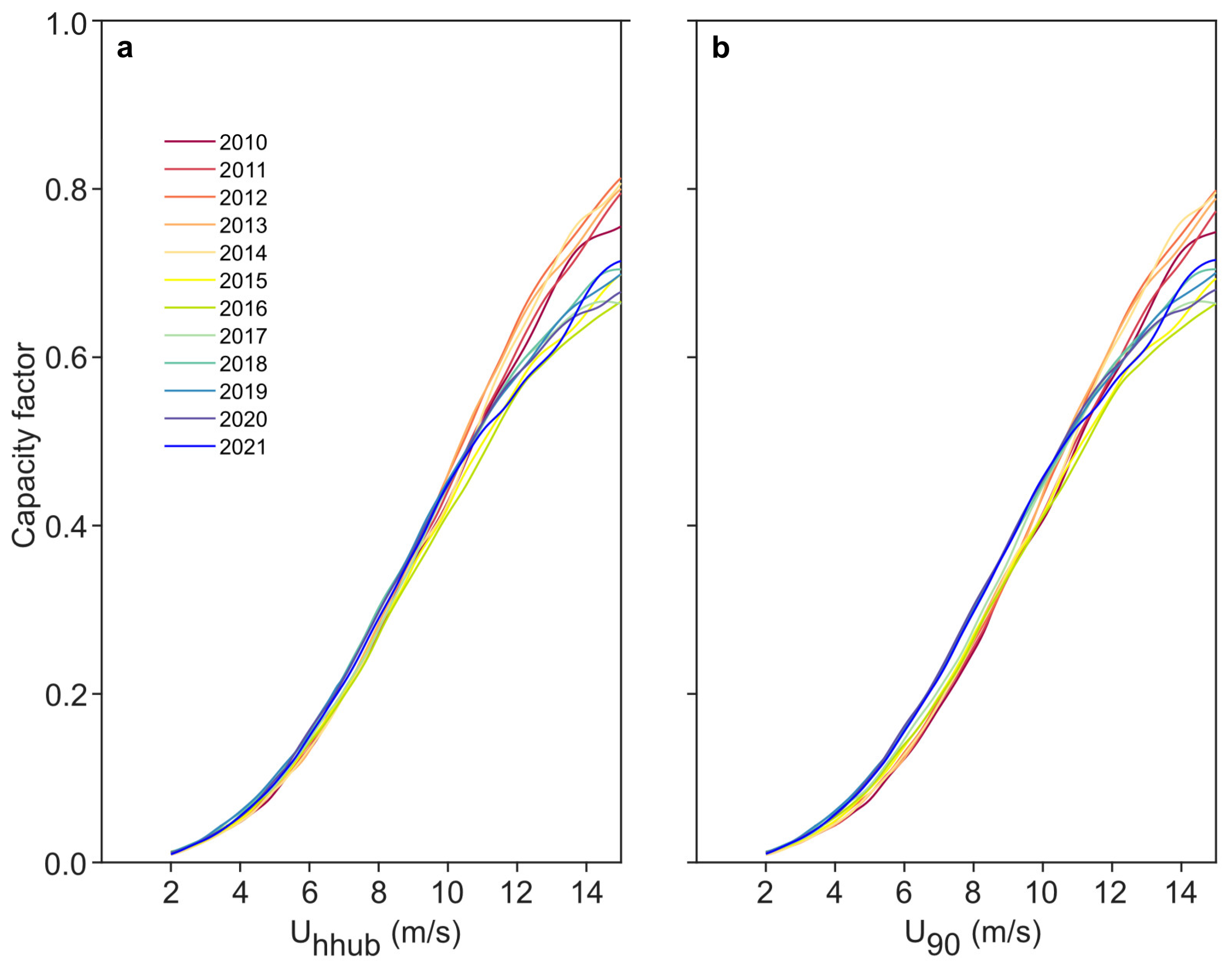
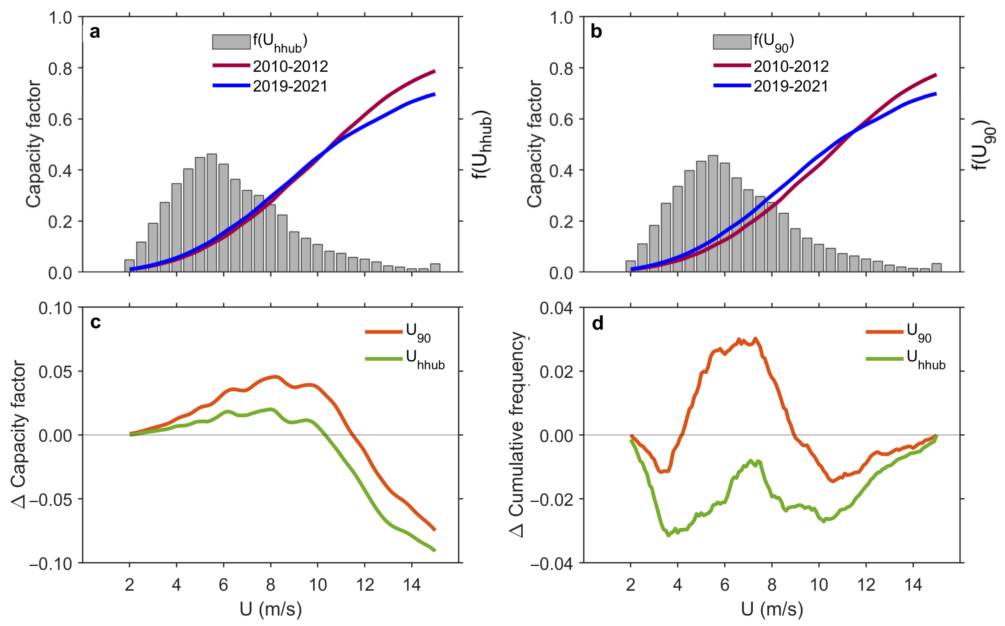
3.2. National Power Curves

Figure 5 shows the national power curves for 2010–2021 as functions of U_hhub. The goodness-of-fit of the splines is always on a high level. The R² values varied between 0.94 for 2010 and 0.98 for 2015. The spline fitting accuracy is slightly worse in the years up to 2013 than since 2014. Regardless of the year, all of the CF curves have a sigmoidal shape. It reveals that even when considering all wind turbines in a country, the power curves have similar characteristics as those of individual wind turbines. However, there are relevant variations between years, considering the power curve details. CF variations between years appear for all U_hhub classes. The CF values of low U_hhub classes have generally increased, which underlines that modern wind turbines can use weak wind resources better [20]. For instance, at a U_hhub of 5.0 m/s, the CF ranged between 0.083 for 2010 and 0.102 for 2019. As of 2015, the CF values are always higher than 0.09, but before that, they were usually lower. A CF increase is also noticeable for medium U_hhub classes. Before 2018, CF for U_hhub = 8.0 m/s was about 0.28. Since 2018, CF values are always around 0.30. As for U_hhub > 10.0 m/s, the higher CF values occurred in the early years. One reason is the increase in the CUE. The national power curve flattens at the upper tail due to increased shutdowns of wind turbines during periods of high OWE. Such a plateau of national power curves was evident in 2017, 2018, and 2021.

Figure 6 summarizes the national power curves for 2010–2021 as functions of the U_hhub (Figure 6a) and U₉₀ (Figure 6b). The CF development as a function of U_hhub between 2010–2021 indicates the influences of technical wind turbine improvement. In contrast, the power curves of U₉₀ additionally reflect the hhub increase. Both power curve variants show a CF increase during low to medium U_hhub classes and a CF decrease during high U_hhub classes. The annual differences between the U₉₀ power curves are more pronounced during low and medium U classes than for the U_hhub power curves. At a U₉₀ of 5.0 m/s, the CF lies between 0.074 for 2010 and 0.103 for 2019. At a moderate U₉₀ of 8.0 m/s, the CF is 0.251 for 2010 and 0.305 for 2020. The annual differences between the U₉₀ power curves are less than for the U_hhub power curves in the high U range. However, they are still relevant. When U₉₀ is 14.0 m/s, the CF exceeds 0.70 before 2015. Afterward, CF is less than 0.70 at the same U₉₀ class.

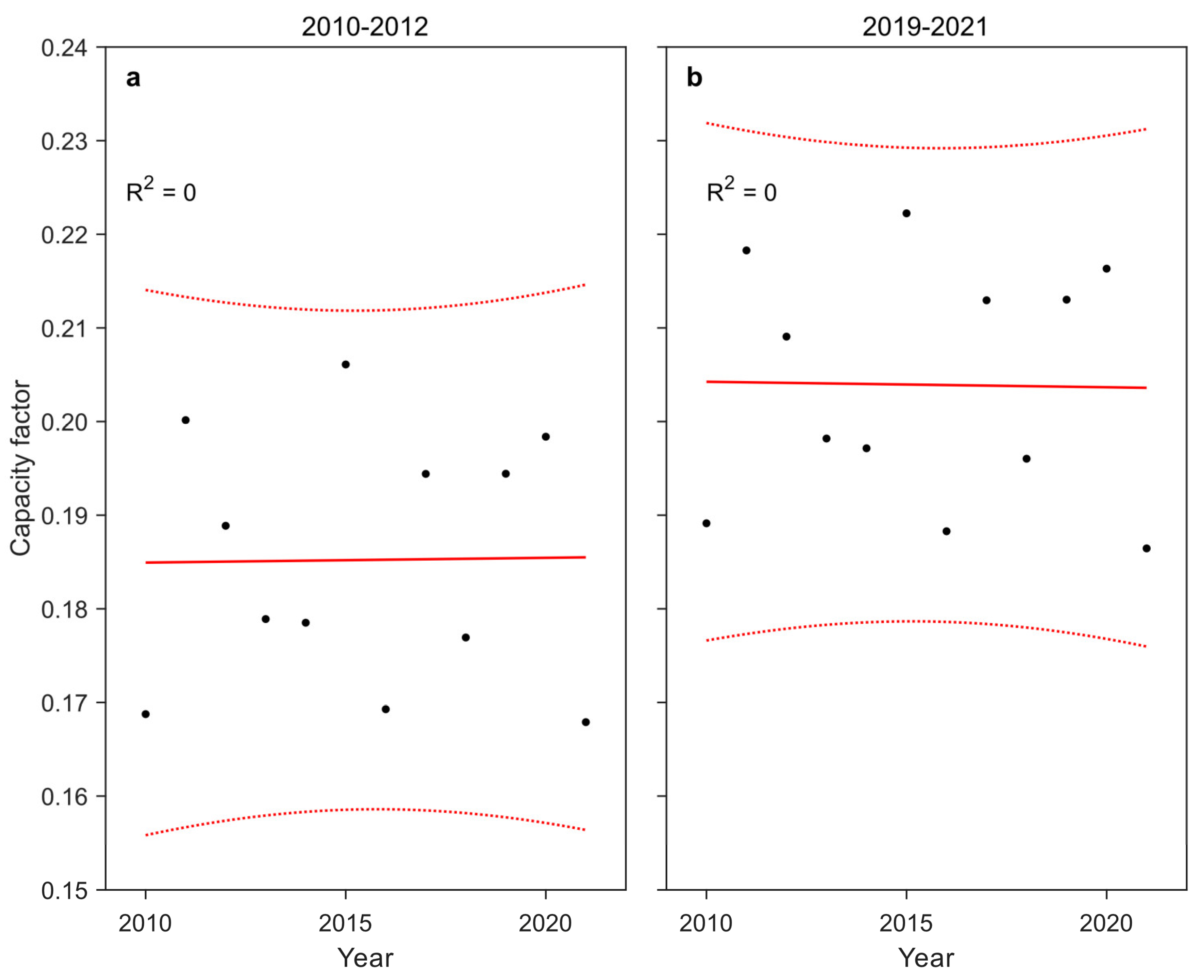
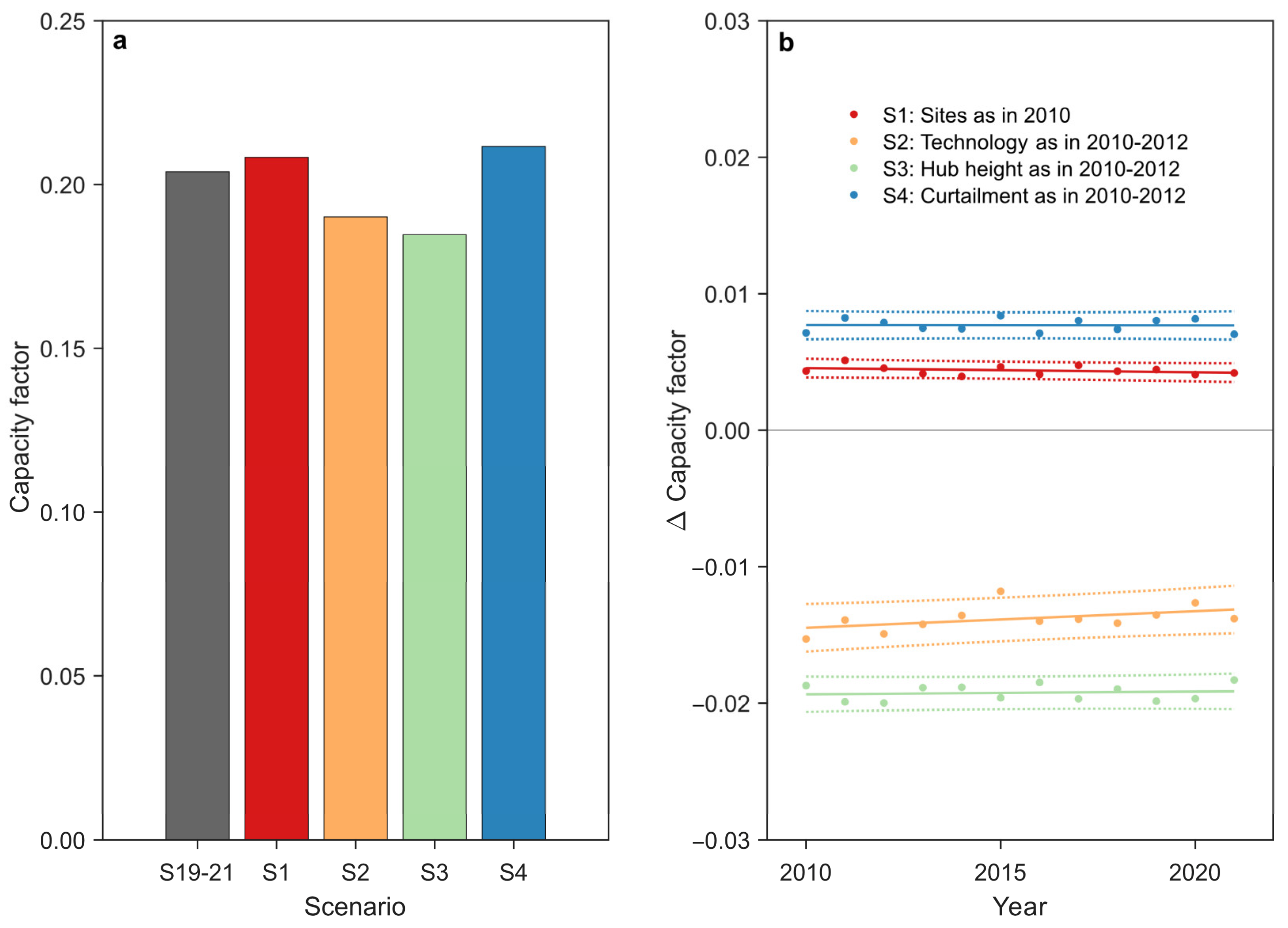
3.3. Shares of the Drivers in CF Development

Singular events may influence the power curves of individual years. Thus, Figure 7 compares the properties of the mean national power curves in 2010–2012 with 2019–2021. It also considers the differences between the U₉₀ (Figure 7a) and U_hhub (Figure 7b) power curve variants. This representation is the basis for quantifying the shares of the drivers in CF development. In addition, the figures present the U₉₀ and U_hhub probability density functions (f(U)) to emphasize the relevant U classes for wind turbine power output. The most frequent U_hhub and U₉₀ class (width 0.5 m/s) is 5.5 m/s. The high f(U) values extend from ≈4.0 to ≈8.0 m/s. It underlines that the differences in the power curve variants in the low and medium value range are critical for the wind turbine power output. The f(U) values in the high U range are small. It is consistent with the fact that the number of periods in which curtailment occurs is small. However, as soon as U₉₀ and U_hhub exceed certain limits (about 11.0 m/s), the CUE becomes relevant.

Figure 7c displays the ΔCF between the power curves of 2010–2012 and 2010–2021 for the U_hhub and U₉₀ variants. The highest positive ΔCF values for both power curve variants are at about 8.0 m/s. The ΔCF values are 0.020 for the U_hhub power curve variant and 0.046 for the U₉₀ power curve variant. The total CF increase of 0.046 at about 8.0 m/s consists of technical advancement of wind turbines (0.020) and an hhub increase (0.026). This resulted from the ΔCF differences between the power curve variants. Below 4.0 m/s, the ΔCF is very low because this value range is only slightly above the wind turbine cut-in speed. Above 10.4 m/s for the hhub variant and 11.6 m/s for the U₉₀ variant, the ΔCF becomes negative. In this U value range, the importance of curtailed energy is more critical than the technical improvement of wind turbines and the hhub increase.

Figure 7d presents the difference in cumulative wind speed distributions (ΔF(U)) for U₉₀ and U_hhub. Positive ΔF(U) values indicate a higher non-exceedance probability of U in 2019–2021 than in 2010–2012. Thus, this corresponds to poorer wind resource availability in the specific U range. The ΔF(U) curve for U_hhub is always below 0 due to the hhub increase between 2010–2012 and 2019–2021. At a higher hhub, the U is generally higher. The presentation of ΔF(U) for U₉₀ is a better indicator to estimate the general change in site suitability, since it is independent of the hhub. The ΔF(U) development for U₉₀ reveals a slight decrease in wind resources in the medium wind speed range. The peak is at U₉₀ = 6.6 m/s, being ΔF(U) = 0.030. At low or high U₉₀ values, wind resource availability improved slightly. The negative peak occurs for U₉₀ = 10.6 m/s with ΔF(U) = −0.015.

Figure 8a presents the CF in 2010–2021 with wind turbine fleet properties as they were in 2010–2012. This presentation enables interpretations of the wind resource-driven trend and inter-annual variability of the CF due to the constant wind turbine fleet conditions. The CF inter-annual variability is large. The CF values ranged between 0.168 for 2021 and 0.206 in 2015. There is no CF trend, as hypothesized in the Introduction.

Figure 8b reveals the same presentation but assumes wind turbine fleet properties as they were in 2019–2021. Under these conditions, the CF values lay between 0.186 for 2021 and 0.222 in 2015. A CF trend was also not present. However, the CF values were clearly above the corresponding 2010–2012 values.

Figure 9a shows the mean CF in 2010–2021 under S19–21 and S1–S4. The mean CF in 2019–2021 was 0.204. Assuming S3 reduced the CF to 0.185. Thus, the increase in the hhub is the most crucial cause of CF development in recent years compared to 2010–2012. Changes in wind turbine technology also play a relevant role in the CF increase. Under S2, CF was only 0.190. Changed wind turbine siting and curtailment resulted in CF reduction. The CF value for S1 was 0.208, and for S4, it was 0.212. These results allow calculating the percentage CF change between 2010–2012 and 2019–2021 caused by each driver. Improved wind turbine technology and a rising hhub led to higher CFs by 7.3% and 10.4%, respectively. Less favorable wind turbine sites and curtailment reduced CF by 2.1% and 3.6% compared to 2010–2012, respectively. Considering all four drivers, the CF increase is 11.9%. This value is close to the actual CF increase between the mean of CF in these periods of 11.0%. This result suggests that the four investigated drivers mainly cover all influences on the CF.

Figure 9b shows the annual difference in CF (ΔCF) between S19–21 and S1–S4. It also indicates whether the CF changes vary due to annual variations of the wind resource. The confidence intervals are small for all scenarios. Thus, there is no hint that certain wind resource conditions lead to a principally different driver relevance.

4. Conclusions

We quantified the shares of the main capacity factor drivers (1) wind turbine siting, (2) wind turbine technology, (3) hub height, and (4) curtailed wind energy in perennial capacity factor development. We identified hub height increase as the most relevant driver leading to a higher capacity factor of 10.4% between 2010–2012 and 2019–2021. The second most important capacity factor driver was wind turbine technology causing 7.3% higher capacity factor values. In contrast, wind turbine siting and curtailment moderated the capacity factor increase by 2.1% and 3.6%, respectively. Although we found no multi-year wind resource changes, the capacity factor has enormous inter-annual variability caused by variations in oceanic/atmospheric oscillations. This study did not confirm the hypothesis that the capacity factor increase from 2010 to 2021 was capped by decreasing wind speed due to wind energy expansion.

Based on the results, we recommend that the wind industry should improve wind turbine site quality as much as possible to avoid needless capacity factor reduction. However, the limited availability of high-quality sites and geographical consideration criteria such as distance to urban areas, infrastructure, and access limitations increasingly complicate the finding of suitable sites. Thus, we also recommend a rapid wind turbine fleet transformation to control the capacity factor on the basis of wind turbine features. Countries should continue integrating wind turbines with higher hub heights and improved technical properties with further vigor.

The reinforced wind energy curtailment is a critical blowback of wind energy expansion. The aim must be to minimize the share of curtailed wind energy. Interconnection and battery deployment enable the alleviation of wind energy curtailment. Decision makers should pursue these approaches in tandem with wind energy expansion.

We investigated Germany’s capacity factor development due to its high installed capacity and wind turbine density. Internationally, the results may differ from those of this case study. However, we assume that the relevance of the drivers will be similar in other countries, since the ten countries with the highest installed capacity all have increasing capacity factor values between 2010–2012 and 2018–2020.

The presented methods provide a basis to further investigate recent research questions. Adjusting the national power curves to upcoming wind turbine properties allows the development of wind energy generation scenarios. Future studies may also investigate whether under very high installed wind capacity the large-scale wind resource could decline, leading to reduced capacity factors. A limitation of the presented power curve approach is that no further breakdown of the technical causes of capacity factor development is possible.

References

1. International Renewable Energy Agency. Renewable Energy Statistics 2022. Available online: https://www.irena.org/publications/2022/Jul/Renewable-Energy-Statistics-2022 (accessed on 18 January 2023).
2. International Renewable Energy Agency. Future of Wind. Available online: https://www.irena.org/-/media/files/irena/agency/publication/2019/oct/irena_future_of_wind_2019.pdf (accessed on 18 January 2023).
3. Asadi, M.; Pourhossein, K.; Mohammadi-Ivatloo, B. GIS-assisted modeling of wind farm site selection based on support vector regression. J. Clean. Prod. 2023, 390, 135993. [Google Scholar] [CrossRef]
4. Jung, C.; Schindler, D. Distance to power grids and consideration criteria reduce global wind energy potential the most. J. Clean. Prod. 2021, 317, 128472. [Google Scholar] [CrossRef]
5. Wang, Y.; Qin, Y.; Wang, K.; Liu, J.; Fu, S.; Zou, J.; Ding, L. Where is the most feasible, economical, and green wind energy? Evidence from high-resolution potential mapping in China. J. Clean. Prod. 2022, 376, 134287. [Google Scholar] [CrossRef]
6. Wu, J.; Xiao, J.; Hou, J.; Lyu, X. Development Potential Assessment for Wind and Photovoltaic Power Energy Resources in the Main Desert–Gobi–Wilderness Areas of China. Energies 2023, 16, 4559. [Google Scholar] [CrossRef]
7. Jung, C.; Schindler, D. Integration of small-scale surface properties in a new high resolution global wind speed model. Energy Convers. Manag. 2020, 210, 112733. [Google Scholar] [CrossRef]
8. Jung, C.; Schindler, D. On the inter-annual variability of wind energy generation–A case study from Germany. Appl. Energy 2018, 230, 845–854. [Google Scholar] [CrossRef]
9. Zeng, Z.; Ziegler, A.D.; Searchinger, T.; Yang, L.; Chen, A.; Ju, K.; Piao, S.; Li, L.Z.X.; Ciais, P.; Chen, D.; et al. A reversal in global terrestrial stilling and its implications for wind energy production. Nat. Clim. Chang. 2019, 9, 979–985. [Google Scholar] [CrossRef]
10. Karnauskas, K.B.; Lundquist, J.K.; Zhang, L. Southward shift of the global wind energy resource under high carbon dioxide emissions. Nat. Geosci. 2018, 11, 38–43. [Google Scholar] [CrossRef]
11. Jung, C.; Schindler, D. Development of onshore wind turbine fleet counteracts climate change-induced reduction in global capacity factor. Nat. Energy 2022, 7, 608–619. [Google Scholar] [CrossRef]
12. Gans, F.; Miller, L.M.; Kleidon, A. The problem of the second wind turbine–a note on a common but flawed wind power estimation method. Earth Syst. Dyn. 2012, 3, 79–86. [Google Scholar] [CrossRef] [Green Version]
13. Li, G.; Yan, C.; Wu, H. Onshore wind farms do not affect global wind speeds or patterns. Heliyon 2023, 9, e12879. [Google Scholar] [CrossRef] [PubMed]
14. Gualtieri, G. A comprehensive review on wind resource extrapolation models applied in wind energy. Renew. Sust. Energy Rev. 2019, 102, 215–233. [Google Scholar] [CrossRef]
15. Jung, C.; Schindler, D. The role of the power law exponent in wind energy assessment: A global analysis. Int. J. Energy Res. 2021, 45, 8484–8496. [Google Scholar] [CrossRef]
16. Wu, Y.T.; Liao, T.L.; Chen, C.K.; Lin, C.Y.; Chen, P.W. Power output efficiency in large wind farms with different hub heights and configurations. Renew. Energy 2019, 132, 941–949. [Google Scholar] [CrossRef]
17. Barthelmie, R.J.; Shepherd, T.J.; Pryor, S.C. Increasing turbine dimensions: Impact on shear and power. J. Phys. Conf. Ser. 2020, 1618, 062024. [Google Scholar] [CrossRef]
18. Jung, C.; Schindler, D. On the influence of wind speed model resolution on the global technical wind energy potential. Renew. Sust. Energy Rev. 2022, 156, 112001. [Google Scholar] [CrossRef]
19. Franke, K.; Sensfuß, F.; Deac, G.; Kleinschmitt, C.; Ragwitz, M. Factors affecting the calculation of wind power potentials: A case study of China. Renew. Sust. Energy Rev. 2021, 149, 111351. [Google Scholar] [CrossRef]
20. Martin, S.; Jung, S.; Vanli, A. Impact of near-future turbine technology on the wind power potential of low wind regions. Appl. Energy 2020, 272, 115251. [Google Scholar] [CrossRef]
21. Lacal-Arántegui, R.; Uihlein, A.; Yusta, J.M. Technology effects in repowering wind turbines. Wind Energy 2020, 23, 660–675. [Google Scholar] [CrossRef]
22. Enevoldsen, P.; Xydis, G. Examining the trends of 35 years growth of key wind turbine components. Energy Sustain. Dev. 2019, 50, 18–26. [Google Scholar] [CrossRef]
23. Rinne, E.; Holttinen, H.; Kiviluoma, J.; Rissanen, S. Effects of turbine technology and land use on wind power resource potential. Nat. Energy 2018, 3, 494–500. [Google Scholar] [CrossRef]
24. Hamilton, S.D.; Millstein, D.; Bolinger, M.; Wiser, R.; Jeong, S. How does wind project performance change with age in the United States? Joule 2020, 4, 1004–1020. [Google Scholar] [CrossRef]
25. Lehneis, R.; Thrän, D. Temporally and Spatially Resolved Simulation of the Wind Power Generation in Germany. Energies 2023, 16, 3239. [Google Scholar] [CrossRef]
26. Yun, E.; Hur, J. Probabilistic estimation model of power curve to enhance power output forecasting of wind generating resources. Energy 2021, 223, 120000. [Google Scholar] [CrossRef]
27. Canbulat, S.; Balci, K.; Canbulat, O.; Bayram, I.S. Techno-economic analysis of on-site energy storage units to mitigate wind energy curtailment: A case study in Scotland. Energies 2021, 14, 1691. [Google Scholar] [CrossRef]
28. Weschenfelder, F.; Leite, G.D.N.P.; da Costa, A.C.A.; de Castro Vilela, O.; Ribeiro, C.M.; Ochoa, A.A.V.; Araujo, A.M. A review on the complementarity between grid-connected solar and wind power systems. J. Clean. Prod. 2020, 257, 120617. [Google Scholar] [CrossRef]
29. Moustris, K.; Zafirakis, D. Day-Ahead Forecasting of the Theoretical and Actual Wind Power Generation in Energy-Constrained Island Systems. Energies 2023, 16, 4562. [Google Scholar] [CrossRef]
30. Siddique, M.B.; Thakur, J. Assessment of curtailed wind energy potential for off-grid applications through mobile battery storage. Energy 2020, 201, 117601. [Google Scholar] [CrossRef]
31. Yasuda, Y.; Bird, L.; Carlini, E.M.; Eriksen, P.B.; Estanqueiro, A.; Flynn, D.; Fraile, D.; Lázaro, E.G.; Martín-Martínez, S.; Hayashi, D.; et al. CE (curtailment–Energy share) map: An objective and quantitative measure to evaluate wind and solar curtailment. Renew. Sust. Energy Rev. 2022, 160, 112212. [Google Scholar] [CrossRef]
32. Frysztacki, M.; Brown, T. Modeling curtailment in Germany: How spatial resolution impacts line congestion. In Proceedings of the 17th International Conference on the European Energy Market (EEM) 2020, Stockholm, Sweden, 16–18 September 2019. [Google Scholar]
33. Mehigan, L.; Gallachóir, B.Ó.; Deane, P. Batteries and interconnection: Competing or complementary roles in the decarbonisation of the European power system? Renew. Energy 2022, 196, 1229–1240. [Google Scholar] [CrossRef]
34. Chen, H.; Chen, J.; Han, G.; Cui, Q. Winding down the wind power curtailment in China: What made the difference? Renew. Sust. Energy Rev. 2022, 167, 112725. [Google Scholar] [CrossRef]
35. Wood, D.A. Country-wide solar power load profile for Germany 2015 to 2019: The impact of system curtailments on prediction models. Energy Convers. Manag. 2022, 269, 116096. [Google Scholar] [CrossRef]
36. Federal Network Agency. Marktstammdatenregister. Available online: https://www.marktstammdatenregister.de/MaStR (accessed on 4 May 2022).
37. Jung, C.; Schindler, D. Introducing a new wind speed complementarity model. Energy 2023, 265, 126284. [Google Scholar] [CrossRef]
38. Hersbach, H.; Bell, B.; Berrisford, P.; Hirahara, S.; Horányi, A.; Muñoz-Sabater, J.; Nicolas, J.; Peubey, C.; Radu, R.; Schepers, D.; et al. The ERA5 global reanalysis. Q. J. R. Meteorol. Soc. 2020, 146, 1999–2049. [Google Scholar] [CrossRef]
39. Fraunhofer ISE. Energy-Charts. Available online: https://www.energy-charts.info (accessed on 10 January 2022).
40. Hosking, J.; Wallis, J. Regional Frequency Analysis: An Approach Based on Lmoments; Cambridge University Press: Cambridge, UK, 1997. [Google Scholar]
41. Jung, C.; Schindler, D. Wind speed distribution selection—A review of recent development and progress. Renew. Sust. Energy Rev. 2019, 114, 109290. [Google Scholar] [CrossRef]
42. Morgan, E.C.; Lackner, M.; Vogel, R.M.; Baise, L.G. Probability distributions for offshore wind speeds. Energy Convers. Manag. 2011, 52, 15–26. [Google Scholar] [CrossRef]
43. Copernicus. Complete UERRA Regional Reanalysis for Europe from 1961 to 2019. Available online: https://cds.climate.copernicus.eu/cdsapp#!/dataset/reanalysis-uerra-europe-complete?tab=overview (accessed on 4 May 2022).
44. Cardell, M.F.; Romero, R.; Amengual, A.; Homar, V.; Ramis, C.A. quantile–quantile adjustment of the EURO CORDEX projections for temperatures and precipitation. Int. J. Climatol. 2019, 39, 2901–2918. [Google Scholar] [CrossRef]
45. Jung, C.; Schindler, D. Introducing a new approach for wind energy potential assessment under climate change at the wind turbine scale. Energy Convers. Manag. 2020, 225, 113425. [Google Scholar] [CrossRef]
46. Federal Network Agency and German Federal Cartel Office. Monitoringbericht 2021. Available online: https://www.bundesnetzagentur.de/SharedDocs/Mediathek/Monitoringberichte/Monitoringbericht_Energie2021.pdf?__blob=publicationFile&v=6 (accessed on 10 January 2023).
47. Shokrzadeh, S.; Jozani, M.J.; Bibeau, E. Wind turbine power curve modeling using advanced parametric and nonparametric methods. IEEE Trans. Sustain. Energy 2014, 5, 1262–1269. [Google Scholar] [CrossRef]
Figure 1. National capacity factor (CF) in 2010–2021 (black circles) in terms of (a) annual mean; (b) 3-year mean; and (c) 5-year mean, including the linear trends (red line) with confidence intervals (dotted red line) and the coefficients of determination (R2).
Energies 16 05390 g001
Figure 2. Workflow to quantify the shares of the drivers in capacity factor (CF) development.
Energies 16 05390 g002
Figure 3. Spatial distributions of wind turbine features hub height (hhub), rated power (Pr), and rotor diameter (RD) with (a) hhub in 2010; (b) hhub in 2021; (c) Pr in 2010; (d) Pr in 2021; (e) RD in 2010; (f) RD in 2021. A grid cell has a spatial resolution of 5 km × 5 km and contains the average hhub, Pr, and RD of wind turbines within the grid cell.
Energies 16 05390 g003
Figure 4. Annual courses (black circles) with fitted polynomials (red line) including their 90% prediction bounds (dotted red line) of mean (a) rated power (Pr); (b) hub height (hhub); (c) curtailed wind energy (CUE); (d) wind speed at 90 m (U90). The coefficients of determination (R2) are displayed for the fitted polynomials.
Energies 16 05390 g004
Figure 5. National capacity factor (CF) as a function of wind speed at hub height (Uhhub) in (a) 2010; (b) 2011; (c) 2012; (d) 2013; (e) 2014; (f) 2015; (g) 2016; (h) 2017; (i) 2018; (j) 2019; (k) 2020; (l) 2021. The coefficients of determination (R2) are displayed for the fitted smoothing splines.
Energies 16 05390 g005
Figure 6. National capacity factor (CF) in 2010–2021 (a) as a function of wind speed at hub height (Uhhub); (b) as a function of wind speed at 90 m (U90).
Energies 16 05390 g006
Figure 7. (a) National power curves in 2010–2012 and 2019–2019 as a function of wind speed at hub height (Uhhub) and probability density of Uhhub (f(Uhhub)); (b) national power curves in 2010–2012 and 2019–2019 as a function of wind speed at 90 m (U90) and probability density of U90 (f(U90)); (c) difference between capacity factor (ΔCF) in 2019–2021 and 2010–2012 as a function of wind speed classes (U90, Uhhub); (d) difference of the cumulative frequency classes (ΔF(U)) in 2019–2021 and 2010–2012.
Energies 16 05390 g007
Figure 8. Annual mean national capacity factor (CF) in 2010–2021 (black circles) assuming conditions as in (a) 2010–2012; (b) 2019–2021. The coefficients of determination (R2) are shown for the fitted first degree polynomials (red line), which are presented with 90% confidence intervals (dotted red line).
Energies 16 05390 g008
Figure 9. (a) Mean capacity factor (CF) in 2010–2021 under different scenarios including S19–21 (conditions as in 2019–2021), S1 (sites as in 2010), S2 (technology as in 2010–2012), S3 (hub height as in 2010–2012), and S4 (curtailment as in 2010–2012); (b) differences in CFCF) between S19–21 and the other scenarios (circles) with fitted first degree polynomials (line) and 90% confidence intervals (dotted line).
Energies 16 05390 g009