Performance Analysis of a Millimeter Wave Communication System in Urban Micro, Urban Macro, and Rural Macro Environments

Abstract

The signal power in wireless communication systems is influenced by various factors, including the environment. These factors include path differences, operational frequency, and environmental conditions. Consequently, designing a communication system that generates a stronger signal is highly challenging. To address this, large-scale path-loss models are employed to estimate the path loss and signal power across different frequencies, distances, and environments. In this paper, we focused on the urban micro, urban macro, and rural macro environments to estimate path loss and signal power at millimeter wave frequencies. We compared the path loss and received power among different path-loss models developed by standard organizations. Simulation results indicate that the fifth-generation channel model provides enhanced path loss and signal power in urban micro environments, while the third-generation partnership project model performs well in urban macro and rural macro environments when compared to other path-loss models.

1. Introduction

The wireless communication field is one of the most successful and rapidly expanding industries due to the rising demand for mobile devices, which is followed by network expansion. By the end of 2025, it is estimated that 20 billion devices will be connected to the mobile network, increasing the amount of wireless data traffic [1,2]. Wireless data transfer has also increased as a result of the development of the Internet of Things (IoT), which includes applications for smart cities, smart health care, smart forming, climate monitoring, intelligent transportation, etc. These applications require very high data rates and large bandwidths to design stable and reliable wireless networks [3,4,5]. Therefore, the fifth-generation (5G) wireless networks with millimeter wave (mmWave) frequency (3 GHz–300 GHz) is considered to meet these demands. The mmWave spectrum provides a huge number of underutilized spectrum bands, which will provide high data rates for the expansion of 5G wireless networks. The underused spectrum bands of mmWave offer a great opportunity to extend the coverage capacity and improve the quality of service [6,7,8].

Several studies found that mmWave frequencies have implementation problems, especially with relation to the path loss (PL) and received power (RP) imposed by various parameters such as weather and atmospheric conditions and obstacles in the surroundings [9]. Along with this, the propagating signal is affected by antenna height, location, and type of antenna [10,11,12,13]. Received signal power in a wireless communication system depends on the interference between the signals, spectrum allocation, spectrum efficiency, etc. [14,15]. Therefore, an accurate estimation of signal power and propagation loss is required to design a modern 5G wireless communication system. Analysis of path-loss models at mmWave frequencies is of the highest priority in order to determine the ideal location of 5G base stations (BS). Many researchers and engineers have developed various mmWave propagation models, which include (i) the 5G channel model (5GCM), the 3rd Generation Partnership Project (3GPP), mobile and wireless communication enablers for the twenty-twenty information society (METIS), and millimeter wave-based mobile radio access networks or 5G integrated communication (mmMAGIC) [16,17,18,19].

In this paper, the effectiveness of different existing propagation models such as 5GCM, 3GPP, METIS, and mmMAGIC at mmWave frequencies between 1 and 100 GHz are considered and compared. The urban micro (UMi), urban macro (UMa), and rural macro (RMa) environments were taken into consideration for line-of-sight (LOS) and non-line-of-sight (NLOS) situations. Because the urban microcellular network provides low latency, high capacity, improved coverage, and improved network reliability, urban and rural macrocellular networks provide extended coverage, improved energy efficiency, and cost effective deployments. Out of these three cellular networks, specific deployment strategies can be selected based on factors such as population density, geographic characteristics, and infrastructure availability. The main goals of this paper are to determine the path loss and received power in urban and rural environments, as well as to estimate the PL and RP at different mmWave frequencies using the various path-loss models that are currently available. An optimized path-loss model can be selected based on the estimated path loss and received power in a given environment. The selected optimized model can be used by the service providers to enhance their network capacity and coverage and energy efficiency. The remainder of the paper is structured as follows: Section 2 explains related work, Section 3 discusses path-loss models, Section 4 contains the results and discussions, and Section 5 contains the conclusion.

2. Related Work

The alpha-beta-gamma (ABG) model, the floating intercept (FI) model, and the close-in-free space with distance (CI) model were the three basic path-loss models [20,21]. These models were established using conventional statistical methods or data-dependent machine learning methods. In Ref. [22], machine learning techniques were used to estimate the PL and compare their performance using a random forest, a support vector regression model, and artificial neural networks. The performance of mobile communication systems was calculated and compared using the traditional channel model and the deep learning model at 2.6 GHz [23]. Estimates of propagation loss were made for urban and suburban NLOS scenarios across several frequencies, ranging from 0.8 GHz to 70 GHz [24]. The propagation loss, received power, and PL exponent were estimated for mmWave frequencies using NYUSIM [25]. In an urban LOS scenario at 28 GHz, the PL, PL exponent, and standard deviation were estimated using NYUSIM, which also determined the best direction for signal propagation [26].

Single-frequency CI and FI models and multi-frequency ABG and CIF models were used to evaluate the propagation characteristics of two indoor stairwell environments [27]. The measured results could be utilized for designing an effective indoor communication system and a small-cell wireless network. In Ref. [28], a comparison and analysis of various path-loss models were presented. A PL measurement campaign was conducted in New York City and Austin at 28 GHz and 38 GHz in a UMi environment [29]. From the measurement, it was identified that the shadow factor reduced the PL by 1 dB in New York City and 6 dB in Austin. The improved versions of the CI and FI PL models were considered to measure the mean prediction and standard deviation error for vertical-horizontal and vertical-vertical antenna polarization [21]. The results confirmed that the new versions of the CI and FI models provided better PL compared to the conventional models.

In Ref. [30], the authors compared empirical path-loss models with practical measurements observed at a frequency of 3.5 GHz in Cambridge, UK. They identified that the ECC-33 models produced optimized path loss compared to the Hata and SUI models. In Ref. [31], the authors estimated the path loss using the Hata model and compared it with outdoor measurements. From the comparison, the authors identified the best-optimized path-loss model that yielded the lowest relative error. In Ref. [32], three path-loss models were used to predict the path loss and were compared with the measured data. The authors determined that the Hata model was the best model for path loss prediction in the urban environment. In Ref. [33], the authors conducted measurements of the LOS path loss at frequencies of 3.35 GHz, 8.45 GHz, and 15.75 GHz using the break point distance. Based on the break point distance, they proposed two path loss formulas, one for the lower bound and another for the upper bound of LOS paths in urban micro environments.

In mmWave communication systems, beam management was the major problem due to dense network deployment and directional transmission. Many authors addressed beam management algorithms in the literature to enhance the wireless communication system performance. In Ref. [34], an adaptive beam management algorithm was proposed to enhance privacy protection and to reduce resource conservation. In Ref. [35], hybrid beam-forming scheme was proposed. In this method mmWave spectrum was shared between the multi-beam satellite system and cellular system and maximized the secrecy energy efficiency of the proposed system. In Ref. [36], an optimization scheme was used to maximize the secrecy energy efficiency. The proposed method will enhance security transmission and reduce power consumption. In Ref. [37], the authors proposed a joint beam-forming scheme and optimization scheme for hybrid satellite relay networks to minimize the total transmit power and to enhance the secrecy energy efficiency. A summary of related works is shown in Table 1.

Table 1. Summary of Related Works.

Author & Ref. No.	Frequency	Environment	Observations	Future Scope
Oladimeji, T.T. et al. [21]	24 GHz & 38 GHz	Indoor Environment	An experimental setup was used to estimate the mean prediction error and standard deviation error. These two errors were used to identify the efficiency of improved path-loss models.	Path loss was estimated for a small indoor region, and the authors want to extend it for an outdoor scenario.
Zhang, Y. et al. [22]	2.02 GHz & 5.8 GHz	Urban Scenario	Estimated the path loss using machine learning models.	Collection of training data, incremental learning, and hyper-parameter optimization are the major problems in path loss estimation using machine learning techniques.
Thrane, J. et al. [23]	2.6 GHz	Urban Macro Scenario	Path loss was estimated and compared using traditional channel models and deep learning channel models, and it was observed that the deep learning models provided better path loss compared to the traditional models.	Prediction of path loss using deep learning models is more complex compared to the traditional model.
Nguyen, C. et al. [24]	0.8 GHz to 70 GHz	Urban and Suburban environments	The authors estimated the path loss at mmWave frequencies using a feed-forward deep neural network model. The proposed model enhanced the mean square error and prediction accuracy.	Random search approach was considered for tuning the hyper-parameters.
Hasan, R. et al. [25]	mmWave Bands	UMi, UMa, and RMi environments	MIMO uniform antenna arrays are used to estimate the angle of arrival, angle of departure, and power delay profiles at mmWave frequency bands.	Path loss for different transmitter and receiver distances needs to be calculated for mmWave frequency bands.
Lodro, M.M. et al. [26]	28 GHz	UMi, UMa, and RMa environments	Directional and unidirectional antennas are considered in the urban microcell region, and the angle of arrival, angle of departure, and power delay profiles are estimated.	The authors wanted to extend it for large-scale path-loss models.
Aldhaibani, A.O. et al. [27]	26 GHz, 28 GHz, 32 GHz & 38 GHz	Indoor Stairwell Environment	Path loss, path loss exponent, and standard deviations were estimated for the considered stairwell environments in the indoor region.	Path loss estimation for multi-stair buildings is in the future’s scope.
MacCartney, G.R. et al. [29]	28 GHz & 38 GHz	Urban microcellular environment	The authors estimated path loss in LOS and NLOS scenarios by considering steerable transmitting and receiving antennas in the outdoor environment.	Need to implement it for the mmWave and THz frequency bands.
Roslee, M.B. et al. [31]	400 MHz to 1800 MHz	suburban environment	Existing Hata model was considered to optimize the path loss. System performance is estimated using the relative error.	Path loss estimation and comparison using different path-loss models is needed.
Obot, A. et al. [32]	150 MHz to 1500 MHz	Urban macrocellular environment	Path loss was estimated and compared using the free space, Hata and Egli path-loss models. The authors observed that the Hata model is the best path-loss model out of three models.	Need to implement it for the mmWave and THz frequency bands.
This paper	mmWave Frequency band	Urban Microcell, Urban Macrocell, and Rural Macrocell	In this paper, we estimated and compared path loss using the existing standard path-loss models in the mmWave frequency bands of all possible environments.	Wanted to extend the same in the THz frequency region in the future.

3. Path Loss Models

For accurate design and comparison of wireless networks and for their deployment, wireless channel models are necessary, which will simulate signal propagation accurately and efficiently. In this paper, we considered the existing four path-loss models that are introduced by the four major organizations: (i) 5G channel model (5GCM) [16], (ii) the 3rd Generation Partnership Project (3GPP) [17], (iii) mobile and wireless communication enablers for the twenty-twenty information society (METIS) [18], and (iv) millimeter wave-based mobile radio access networks or 5G integrated communication (mmMAGIC) [19]. The PL in these models depends on the range between transmitter and receiver (T-R), carrier frequency, and environmental conditions. UMi, UMa, and RMa environments under LOS and NLOS scenarios are considered to estimate the PL and RP.

3.1. UMi Path Loss Models

The UMi path-loss model, PL expression, and parameters range, like shadow fading, carrier frequency, distance, and antenna heights, are listed in Table 2. In the UMi environment, the propagation path is divided into two types: street canyon (SC) and open square (OS).

Table 2. UMi Path Loss Models.

Model	PL [dB]	Shadow Fading [dB]	Parameters
5GCM SC LOS	$PL=32.4+21lo{g}_{10}\left(R_{3D}\right)+20lo{g}_{10}\left(f\right)$	$\sigma$ = 3.76	$6$ GHz $<f<100$ GHz
5GCM SC NLOS	CI Model: $PL=32.4+31.7lo{g}_{10}\left(R_{3D}\right)+20lo{g}_{10}\left(f\right)$	$\sigma$ = 8.09	$6$GHz $<f<100$ GHz
	ABG Model: $PL=22.4+35.3lo{g}_{10}\left(R_{3D}\right)+21.3lo{g}_{10}\left(f\right)$	$\sigma$ = 7.82
5GCM OS LOS	$PL=32.4+18.5lo{g}_{10}\left(R_{3D}\right)+20lo{g}_{10}\left(f\right)$	$\sigma$ = 4.2	$6$GHz $<f<100$ GHz
5GCM OS NLOS	CI Model: $PL=32.4+28.9lo{g}_{10}\left(R_{3D}\right)+20lo{g}_{10}\left(f\right)$	$\sigma$ = 7.1	$6$GHz $<f<100$ GHz
	ABG Model: $PL=3.66+41.4lo{g}_{10}\left(R_{3D}\right)+24.3lo{g}_{10}\left(f\right)$	$\sigma$ = 7.0
3GPP SC LOS	$PL-LOS=\left\{\begin{array}{cc}P{L}_1,\hfill & 10m\le R\le d_{BP}\hfill \\ P{L}_2,\hfill & d_{BP}\le R\le 5km\hfill \end{array}\right.$	$\sigma$ = 4.0	$0.5$GHz $<f<100$GHz, $1.5$m $\le h_2\le 22.5$ m
	$P{L}_1=32.4+21lo{g}_{10}(R_{3D}+20lo{g}_{10}\left(f\right)$		$h_1$ = 10 m
	$P{L}_2=32.4+40lo{g}_{10}(R_{3D}+20lo{g}_{10}\left(f\right)-9.5lo{g}_{10}({\left(d_{BP}\right)}^2$$+{(h_1-h_2)}^2)$
	where $d_{BP}$ is a break point distance, which is given by Equation (1).
3GPP SC NLOS	$PL=max(PL-LOS,PL-NLOS)$	$\sigma =7.82$	$0.5$GHz $<f<100$ GHz
	$PL-NLOS=22.4+35.3lo{g}_{10}\left(R_{3D}\right)+21.3lo{g}_{10}\left(f\right)$$-0.3(h_2-1.5)$		$10$m$<R<5000$ m, $1.5$m $\le h_2\le 22.5$ m, $h_1$ = 10 m
METIS SC LOS	$PL-LOS=\left\{\begin{array}{cc}P{L}_1,\hfill & 10m\le R\le d_{BP1}\hfill \\ P{L}_2,\hfill & d_{BP1}\le R\le 500m\hfill \end{array}\right.$	$\sigma$ = 3.1	$0.8$GHz $<f<60$ GHz, $1.5$m $\le h_2\le 22.5$ m
	$P{L}_1=28.0+22lo{g}_{10}(R_{3D}+20lo{g}_{10}\left(f\right)+P{L}_0$		$h_1$ = 10 m
	$P{L}_2=7.8+40lo{g}_{10}(R_{3D}+2lo{g}_{10}\left(f\right)-18lo{g}_{10}\left(h_1{h}_2\right)$$+P{L}_1\left(d_{BP}\right)$
	where $d_{BP1}$ and $P{L}_0$ are given by Equations (2) and (3)
METIS SC NLOS	$PL=max(PL-LOS,PL-NLOS)$	$\sigma =4.0$	$0.45$GHz $\le f\le 6$ GHz
	$PL-NLOS=23.15+36.7lo{g}_{10}\left(R_{3D}\right)+26lo{g}_{10}\left(f\right)$$-0.3\left(h_2\right)$		$10$m $<R<2000$ m, $1.5$m $\le h_2\le 22.5$ m, $h_1$ = 10 m
mmMAGIC SC LOS	$PL=32.9+19.2lo{g}_{10}\left(R_{3D}\right)+20.8lo{g}_{10}\left(f\right)$	$\sigma$ = 2.0	$6$GHz $<f<100$ GHz
mmMAGICSC NLOS	$PL=31.0+45lo{g}_{10}\left(R_{3D}\right)+20lo{g}_{10}\left(f\right)$	$\sigma$ = 7.82	$6$GHz $<f<100$ GHz

Note: R, $R_{3D}$, $h_1$ and $h_2$ are in meters, frequency (f) is in GHz and path loss (PL) is in dB.

3.1.1. 5GCM Model

The large-scale CI with reference distance and ABG models are considered to estimate the PL and RP in LOS and NLOS scenarios. In 5GCM, urban micro-street canyon (UMi-SC) and urban micro-open square (UMi-OS) environments are considered, and PL and RP for these models under LOS and NLOS scenarios are estimated at a frequency range of 6 GHz to 100 GHz. The PL equations of the 5GCM model are shown in Table 1.

3.1.2. 3GPP Model

In this model, the distance $\left(R_{3D}\right)$ between transmitter and receiver (T-R) is estimated based on antenna heights and R, which is given by $\sqrt{{\left(R\right)}^2+{(h_1-h_2)}^2}$[19]. Where R is the actual distance between T and R, $h_1$ and $h_2$ are the actual BS and user equipment antenna heights, respectively. In a 3GPP LOS scenario, PL is estimated based on break point distance $\left(d_{BP}\right)$, i.e., if $R<d_{BP}$ then $P{L}_1$ otherwise, $P{L}_2$ is used to estimate the PL using the large-scale CI model [38,39,40]. Break point distance is estimated as [41]

$$\begin{array}{c}\hfill d_{BP}=4h_{11}{h}_{21}f\times {10}^9/c\\ \hfill h_{11}=h_1-1.0\mathrm{m}\\ \hfill h_{21}=h_2-1.0\mathrm{m}\end{array}$$

(1)

where $h_{11}$ and $h_{21}$ are effective antenna heights and c is the velocity of free space 3 ×${10}^8$ m/s.

Large scale ABG model is used to estimate the PL of UMi-NLOS scenario [19].

3.1.3. METIS Model

LOS PL of METIS model depends on break point distance ($d_{BP1}$) and path loss offset ($P{L}_0$). $d_{BP1}$ and $P{L}_0$ are given by [18]

$$\begin{array}{c}\hfill d_{BP}=0.87exp\left(\frac{-lo{g}_{10}\left(f\right)}{0.65}\right)\times \frac{4\left(h_{11}\right)\left(h_{21}\right)f\times {10}^9}{c}\end{array}$$

(2)

$$\begin{array}{ccc}\hfill P{L}_0\left[dB\right]& =& -1.38lo{g}_{10}\left(f\right)+3.34\hfill \end{array}$$

(3)

The large-scale ABG model is used to estimate the PL in UMI-NLOS scenario.

3.1.4. mmMAGIC Model

This model uses large-scale ABG model to estimate the PL in UMi-LOS and UMi-NLOS scenarios.

3.2. UMa Path Loss Models

The large-scale PL of an urban macro environment is measured using 5GCM, 3GPP, and METIS models. The PL model, PL expression, standard deviation, and various parameters like carrier frequency, distance, and antenna heights are listed in Table 3.

Table 3. UMa Path Loss Models.

Model	PL [dB]	Shadow Fading [dB]	Parameters
5GCM LOS	$PL=32.4+20lo{g}_{10}\left(R_{3D}\right)+20lo{g}_{10}\left(f\right)$	$\sigma$ = 4.1	$6$GHz $<f<100$ GHz
5GCM NLOS	CI Model: $PL=32.4+30lo{g}_{10}\left(R_{3D}\right)+20lo{g}_{10}\left(f\right)$	$\sigma$ = 6.8	$6$GHz $<f<100$ GHz
	ABG Model: $PL=19.2+34lo{g}_{10}\left(R_{3D}\right)+23lo{g}_{10}\left(f\right)$	$\sigma$ = 6.5
3GPP LOS	$PL-LOS=\left\{\begin{array}{cc}P{L}_1,\hfill & 10m\le R\le d_{BP}\hfill \\ P{L}_2,\hfill & d_{BP}\le R\le 5km\hfill \end{array}\right.$	$\sigma$ = 6.0	$0.5$GHz $<f<100$ GHz, $1.5$m $\le h_2\le 22.5$ m
	$P{L}_1=28+22lo{g}_{10}(R_{3D}+20lo{g}_{10}\left(f\right)$		$h_1$ = 25 m
	$P{L}_2=28+40lo{g}_{10}(R_{3D}+20lo{g}_{10}\left(f\right)-9lo{g}_{10}({\left(d_{BP}\right)}^2+{(h_1-h_2)}^2)$
	where $d_{BP}$ is a break point distance, which is given by Equation (1).
3GPP NLOS	$PL=max(PL-LOS,PL-NLOS)$	$\sigma =6$	$0.5$GHz $<f<100$ GHz
	$PL-NLOS=13.54+39.08lo{g}_{10}\left(R_{3D}\right)+20lo{g}_{10}\left(f\right)-0.6(h_2-1.5)$		$10$m $<R<5000$ m, $1.5$m $\le h_2\le 22.5$ m, $h_1$ = 25 m
METIS LOS	$PL-LOS=\left\{\begin{array}{cc}P{L}_1,\hfill & 10m\le R\le d_{BP1}\hfill \\ P{L}_2,\hfill & d_{BP1}\le R\le 5km\hfill \end{array}\right.$	$\sigma$ = 4	$0.45$GHz $<f<6$ GHz, $1.5$m $\le h_2\le 22.5$ m
	$P{L}_1=28+22lo{g}_{10}(R_{3D}+20lo{g}_{10}\left(f\right)$		$h_1$ = 25 m
	$P{L}_2=28+40lo{g}_{10}(R_{3D}+20lo{g}_{10}\left(f\right)-9lo{g}_{10}({\left(d_{BP}\right)}^2+{(h_1-h_2)}^2)$
	where $d_{BP1}$ is given by Equation (1)
METIS NLOS	$PL=max(PL-LOS,PL-NLOS)$	$\sigma =6.0$	$0.45$GHz $\le f\le 6$ GHz
	$PL-NLOS=161.94+(43.42-3.1lo{g}_{10}\left(h_1\right))(lo{g}_{10}\left(R_{3D}\right)-3)$$+20lo{g}_{10}\left(f\right)-0.6\left(h_2\right)-7.1lo{g}_{10}\left(w\right)+7.5lo{g}_{10}\left(h\right)$$-\left(24.37-3.7{\left(\frac{h}{h_1}\right)}^2\right)lo{g}_{10}\left(h_1\right)$		$10$m $<R<2000$ m, $1.5$m $\le h_2\le 22.5$ m, $h_1$ = 25 m, w = 20 m, h = 20 m

3.2.1. 5GCM Model

CI and ABG large-scale path-loss models are used to measure the PL in an urban macro environment [14,36,42]. In a UMa environment, the BS antenna height is 25 m, which is higher than the UMi case. This will help reduce the PL by avoiding obstructions below 25 m height from the ground surface [19].

3.2.2. 3GPP Model

The LOS UMa PL is measured based on the break point distance and the ABG large-scale path-loss model. Similarly, UMa NLOS PL is measured using the ABG model for a standard deviation of 7.8 dB [17].

3.2.3. METIS Model

In this model, LOS and NLOS PL is measured using the large-scale ABG model [18].

3.3. RMa Path Loss Models

The PL in a rural macro environment is measured using ITU-RM.2135/3GPP TR 38.901 [43,44]. The PL and its parameters are listed in Table 4.

Table 4. RMa Path Loss Models.

Model	PL [dB]	Shadow Fading [dB]	Parameters
3GPP LOS	$PL-LOS=\left\{\begin{array}{cc}P{L}_1,\hfill & 10m\le R\le d_{BP2}\hfill \\ P{L}_2,\hfill & d_{BP2}\le R\le 10km\hfill \end{array}\right.$		$0.5$GHz $<f<100$ GHz, $1$m $\le h_2\le 10$ m
	$\begin{array}{c}P{L}_1=20lo{g}_{10}(40\pi R_{3D}f/3)+min(0.03h^{1.72},10)lo{g}_{10}\left(R_{3D}\right)-\hfill \\ min(0.044h^{1.72},14.77)+0.002lo{g}_{10}\left(h\right)R_{3D}\hfill \end{array}$	$\sigma$ = 4.0	$h_1$ = 35 m, h = 5 m
	$P{L}_2=P{L}_1\left(d_{BP2}\right)+40lo{g}_{10}(R_{3D}/d_{BP2})$	$\sigma =8$
	where $d_{BP2}$ is a break point distance, which is given by Equation (4).
3GPP NLOS	$PL=max(PL-LOS,PL-NLOS)$	$\sigma =8$	$0.5$GHz $<f<100$ GHz
	$\begin{array}{c}PL-NLOS=161.94+(43.42-3.1lo{g}_{10}\left(h_1\right))(lo{g}_{10}\left(R_{3D}\right)-3)+\hfill \\ 20lo{g}_{10}\left(f\right)-(3.2{\left(lo{g}_{10}\left(11.75h_2\right)\right)}^2-4.97)-7.1lo{g}_{10}\left(w\right)+\hfill \\ 7.5lo{g}_{10}\left(h\right)-\left(24.37-3.7{\left(\frac{h}{h_1}\right)}^2\right)lo{g}_{10}\left(h_1\right)\hfill \end{array}$		$10$m $<R<5000$ m, $1$m $\le h_2\le 10$ m, $h_1=35$m$,w=20$m, $h=5$ m

3GPP Model

The large-scale CI model is used to measure the LOS RMa path loss [43,44]. LOS path loss is estimated based on the break point distance and it is given by

$$d_{BP2}=2\pi h_1{h}_{2}f/c$$

(4)

The received signal power in UMi, UMa and RMa environments is estimated by [45]

$$RP=\frac{G_t{G}_r{P}_t}{K{T}_s\Gamma \left(PL\right)(E_b/N_0)}$$

(5)

where $G_t$, $G_r$ are transmitter and receiver antenna gains, respectively, $P_t$ is transmitter power, K is a Bolztman’s constant, $PL$ is the path loss due to various environments, $T_s$ is noise temperature, $\Gamma$ is the data rate and $E_b/N_0$ is the ratio of energy per bit to noise spectral density.

4. Results and Discussion

The path loss and received power are influenced by a wide range of variables since each model is unique in its design and features depending on the kind of operating environment it is used in. In this paper, PL and RP are estimated for urban and rural environments, respectively. The simulation results of the UMi, UMa, and RMa environments for mmWave frequencies are presented and analyzed in this section. PL and RP are estimated using the various path-loss models proposed by the standard organizational bodies. Figure 1, Figure 2, Figure 3, Figure 4, Figure 5, Figure 6, Figure 7, Figure 8 and Figure 9 compare the PL of UMi, UMa, and RMa environments using various models at underutilized mmWave frequency bands of 28 GHz, 38 GHz, 60 GHz and 75 GHz, respectively. It has been found that the measured PL is affected by the distance (R), carrier frequency (f), and height of the BS antenna $\left(h_1\right)$.

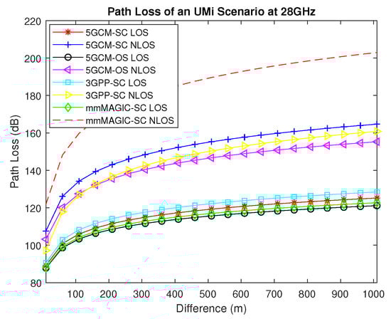
Figure 1. Path loss of an Urban Micro environment at 28 GHz.

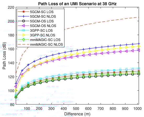
Figure 2. Path loss of an Urban Micro environment at 38 GHz.

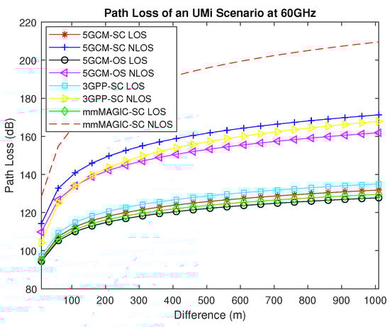
Figure 3. Path loss of an Urban Micro environment at 60 GHz.

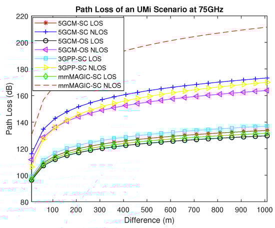
Figure 4. Path loss of an Urban Micro environment at 75 GHz.

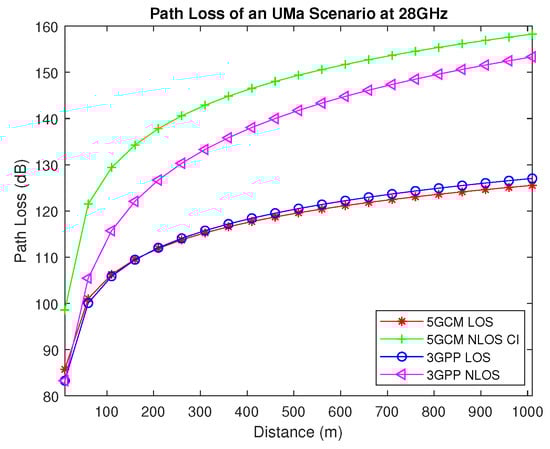
Figure 5. Path loss of an Urban Macro environment at 28 GHz.

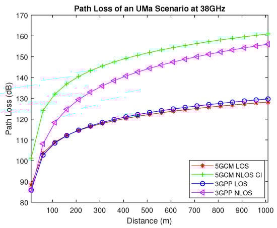
Figure 6. Path loss of an Urban Macro environment at 38 GHz.

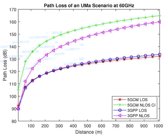
Figure 7. Path loss of an Urban Macro environment at 60 GHz.

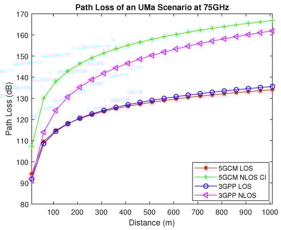
Figure 8. Path loss of an Urban Macro environment at 75 GHz.

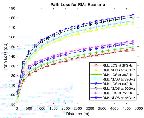
Figure 9. Path loss of Rural Macro environment.

4.1. Path Loss Estimation

Path loss in urban micro, urban macro, and rural macro environments are estimated using the equations shown in Table 1, Table 2 and Table 3. Figure 1, Figure 2, Figure 3 and Figure 4 present the measurement and comparison of path loss in the UMi scenario across different frequencies: 28 GHz, 38 GHz, 60 GHz, and 75 GHz. Among the models, the line-of-sight 5GCM-OS model demonstrates lower path loss, as shown by the findings in Figure 1, Figure 2, Figure 3 and Figure 4. Notably, the line-of-sight mmMAGIC model closely resembles the path loss curve observed in the 5GCM-OS model. In non-line-of-sight propagation, the path loss of 5GCM-OS is slightly higher than that of the 3GPP-SC model for distances less than 150 m, equal at a distance of 150 m, and higher than 3GPP-SC for distances greater than 150 m. Consequently, 5GCM-OS exhibits the lowest path loss beyond 150 m, while 3GPP-SC yields the lowest path loss up to that point. The mmMAGIC-SC model generates the highest path loss in the NLOS scenario.

It can be seen from Figure 1, Figure 2, Figure 3 and Figure 4 that each model’s path loss gradually rises with distance and frequency. The 5GCM-OS model exhibits the lowest path loss in both LOS and NLOS scenarios for mmWave frequencies at various distances when compared to other models. Among them, the 3GPP-SC and mmMAGIC-SC models yield the highest path loss in LOS and NLOS scenarios, respectively. In practical applications, network providers seek higher signal power and lower path loss. In the UMi scenario, the 5GCM model produces the least path loss in LOS and NLOS scenarios at variable frequencies and distances. Therefore, the 5GCM model is considered to be an optimal path-loss model, with an optimal distance of 150 m in urban micro scenarios. Table 5 displays the PL values for each model at various frequencies.

Table 5. Path Loss of UMi, UMa and RMa environments at 28 GHz, 38 GHz, 60 GHz and 75 GHz.

Model	PL [dB] at R = 100 m				PL [dB] at R = 500 m				PL [dB] at R = 1000 m
	28	38	60	75	28	38	60	75	28	38	60	75
Urban Micro Environment
5GCM-SC LOS	106.7	108.6	112.6	114.5	119.2	121.9	125.9	127.8	125.2	127.8	131.8	133.7
5GCM-OS LOS	104.2	106.0	109.9	111.9	115.6	118.3	123.3	124.2	121.1	123.8	127.7	129.7
3GPP-SC LOS	108.2	110.9	114.9	116.8	122.2	124.8
	128.8	130.8	128.4	131.1	135.1	136.9
mmMAGIC-SC LOS	104.8	107.0	111.1	113.1	116.9	119.7	123.9	125.9	122.6	125.1	129.6	131.8
5GCM-SC NLOS	134.2	136.9	140.8	142.8	155.2	157.9	161.9	163.8	164.7	167.3	171.3	173.2
5GCM-OS NLOS	127.3	129.8	133.9	136.0	146.7	149.3	153.3	155.3	156.4	157.9	161.9	163.8
3GPP-SC NLOS	126.9	129.7	133.9	136.0	150.4	153.2	157.2	159.4	160.8	163.7	167.8	169.9
mmMAGIC-SC NLOS	159.7	162.4	166.4	168.3	189.6	192.3	196.2	198.2	203.4	205.6	209.6	211.5
Urban Macro Environment
5GCM LOS	106.1	108.9	112.9	114.5	119.6	122.2	126.2	128.2	125.5	128.2	132.1	134.1
3GPP LOS	105.9	108.5	112.5	114.4	120.5	123.2	127.2	129.1	127.0	129.7	133.7	135.6
5GCM NLOS	129.2	132.0	136.0	137.9	19.3	152.0	155.9	157.9	158.3	160.9	164.9	166.8
3GPP NLOS	115.7	118.3	122.3	124.3	141.8	144.4	148.4	150.3	153.4	156.0	159.9	161.9
Rural Macro Environment
	R = 500 m				R = 1000 m				R = 2000 m
3GPP LOS	120.9	123.6	127.5	129.5	127.7	130.3	134.3	136.2	135.2	137.9	141.8	143.8
3GPP NLOS	136.5	139.1	143.1	145.0	147.9	150.6	154.6	156.5	159.5	162.1	166.1	168.0

Figure 5, Figure 6, Figure 7 and Figure 8 measure and compare the PL of the urban macro environment at 28 GHz, 38 GHz, 60 GHz, and 75 GHz, respectively. Compared to other models, the line-of-sight 5GCM model produces less path loss, which can be observed in Figure 5, Figure 6, Figure 7 and Figure 8. The line-of-sight 3GPP path loss curve closely resembles the path loss in the LOS 5GCM model. In LOS propagation, the path loss of 5GCM is slightly higher than the path loss of 3GPP model if the distance is less than 300 m, it is equal at a distance of 300 m, and if the distance is greater than 300 m, the path loss of 3GPP is higher than the path loss of 5GCM. Therefore, 5GCM creates the lowest path loss after 300 m while 3GPP generates the lowest path loss up to that point. The highest path loss is produced by the 5GCM model in the NLOS scenario.

It can be seen from Figure 5, Figure 6, Figure 7 and Figure 8 that each model’s path loss gradually rises with distance and frequency. In comparison to the other models, the 5GCM and 3GPP model generates the lowest path loss in LOS and NLOS scenarios, respectively, and these two models are assumed as optimal path-loss models and the optimal distance is 300 m in urban macro scenarios. The detailed PL values at various frequencies are listed in Table 6.

Table 6. Summary of Path loss models.

Parameter	5GCM Model	3GPP Model	METIS Model	mmMAGIC Model
Path Loss in UMi	This model provides the least path loss in LOS and NLOS Scenarios	This model provides highest path loss in LOS scenario		This model provides highest path loss in NLOS Scenario
Path Loss in UMa	This model provides the least path loss in LOS	This model provides least path loss in NLOS scenario
Path Loss in RMa		Only the 3GPP model is used to estimate the path loss in rural macro cellular networks
Advantages	This model is specifically designed for 5G networks, incorporating unique characteristics associated with 5G frequency bands and technologies	This model utilizes a standardized approach for path loss estimation in cellular networks and also 5G networks	This model is specifically designed to estimate spectral efficiency, energy efficiency, improved coverage, and path loss in 5G networks	This model is specifically designed for 5G networks and it addresses challenges and opportunities of mmWave frequency bands.
	This model accurately estimates the path loss in urban micro and macro environments	This model estimates the path loss for a wide range of propagation environments and scenarios.	This model accurately estimates the path loss in urban micro and macro environments	This model accurately estimates the path loss in urban micro and indoor environments
Disadvantages	It does not support non-mmWave frequency Bands	This model does not consider all the real-world problems while estimating the path loss	operating frequency range is very small and above 6 GHz it does not support	It does not support non-mmWave frequency Bands
	This model is not well-suited for rural environments	This model lacks accuracy in predicting path loss within real-world environments	This model is not well-suited for urban macro rural macro environments	This model is not well-suited for urban macro rural macro environments

Figure 9 measure and compare the PL of the rural macro environment at 28 GHz, 38 GHz, 60 GHz, and 75 GHz. It can be seen from Figure 9 and Table 4 that path loss gradually rises with distance and frequency.

Path loss in urban micro cells and urban and rural macro cells can be affected by various factors such as distance, obstacles, interference, base station antenna height, and frequency band. Observations from Figure 1, Figure 2, Figure 3, Figure 4, Figure 5, Figure 6, Figure 7, Figure 8 and Figure 9 are that the PL in urban micro cells is generally higher than in urban macro and rural macro cells due to the lower base station antenna height. The base station antenna height in urban and rural macro cells is generally higher than that of an urban micro cell due to the difference in their coverage areas and signal propagation characteristics.

Macro cells generally possess a larger coverage area compared to micro cells, requiring base stations to transmit signals over greater distances to cover equivalent regions. By placing the antenna at a considerable distance from the ground, signals can traverse longer distances and cover wider areas. Nevertheless, signal loss can occur in both cell site types due to interference and obstructions, with the extent of loss contingent on the specific deployment and environmental conditions. Therefore, 5GCM and 3GPP models are considered to be optimal path-loss models in urban micro and macro, rural macro environments at an optimal distance of 150 m and 300 m, and 1000 m, respectively. From the simulation results, the advantages and disadvantages of each path-loss model are listed in Table 6.

4.2. Received Power Estimation

Received power in urban micro, urban macro, and rural macro environments are estimated using Equation (5). Figure 10, Figure 11, Figure 12 and Figure 13 measure and compare the received power of UMi scenario at 28 GHz, 38 GHz, 60 GHz, and 75 GHz, respectively. Compared to other models, the 5GCM-OS model produces the highest signal power in LOS scenario, which will be observed from Figure 10, Figure 11, Figure 12 and Figure 13. The line-of-sight mmMAGIC curve closely resembles the 5GCM-OS model. In NLOS propagation, the received power of 5GCM-OS is slightly lower than the received power of 3GPP-SC if the distance is less than 150 m, it is equal at a distance of 150 m, and if the distance is greater than 150 m, the received power of 3GPP-SC is lower than the received power of 5GCM-OS model. Therefore, 5GCM-OS creates the highest received power after 150 m while 3GPP-SC generates the highest received up to that point. The lowest received power is produced by the mmMAGIC-SC model in the NLOS scenario.

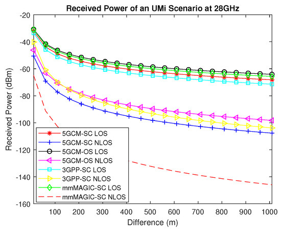
Figure 10. Received power of an Urban Micro environment at 28 GHz.

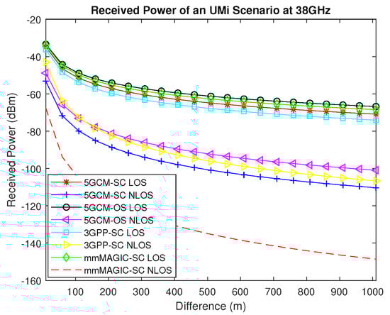
Figure 11. Received power of an Urban Micro environment at 38 GHz.

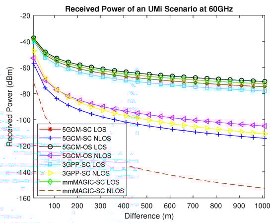
Figure 12. Received power of an Urban Micro environment at 60 GHz.

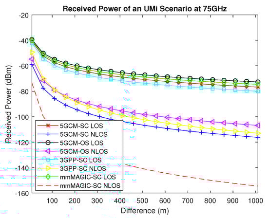
Figure 13. Received power of an Urban Micro environment at 75 GHz.

It can be seen from Figure 10, Figure 11, Figure 12 and Figure 13 that each model’s received power gradually reduces with distance and frequency. In comparison to the other models, the 5GCM-OS model generates the highest power in LOS and NLOS scenarios. The minimum power is produced by the 3GPP-SC and mmMAGIC-SC models, respectively. Table 7 displays the RP values for each model at various distances and frequencies.

Table 7. Received Power of UMi, UMa, and RMa environments at 28 GHz, 38 GHz, 60 GHz, and 75 GHz.

Model	PL [dB] at R = 100 m				PL [dB] at R = 500 m				PL [dB] at R = 1000 m
	28	38	60	75	28	38	60	75	28	38	60	75
Urban Micro Environment
5GCM-SC LOS	−48.9	−51.6	−55.6	−57.5	−62.2	−64.9	−68.8	−70.8	−68.2	−70.8	−74.8	−76.7
5GCM-OS LOS	−46.4	−49.0	−53.0	−54.9	−58.6	−61.3	−65.3	−67.2	−64.1	−66.8	−70.7	−72.7
3GPP-SC LOS	−51.2	−53.9	−57.9	−59.8	−65.2	−67.9	−71.8	−73.8	−71.4	−74.1	−78.1	−80.0
mmMAGIC-SC LOS	−47.2	−50.0	−53.1	−56.1	−59.9	−62.7	−66.8	−68.9	−65.7	−68.4	−72.6	−74.6
5GCM-SC NLOS	−77.2	−79.9	−83.8	−85.8	−98.3	−100.9	−104.9	−106.8	−107.7	−110.3	−114.3	−116.2
5GCM-OS NLOS	−69.9	−73.3	−76.9	−79.0	−89.7	−92.3	−96.3	−98.2	−98.3	−100.9	−104.9	−106.8
3GPP-SC NLOS	−70.5	−72.7	−76.9	−79.0	−93.4	−96.2	−100.4	−102.5	−103.8	−106.6	−110.9	−112.9
mmMAGIC-SC NLOS	−102.7	−105.4	−109.3	−111.3	−132.4	−135.3	−139.2	−141.2	−145.9	−148.6	−152.6	−154.5
Urban Macro Environment
5GCM LOS	−49.3	−51.9	−55.9	−57.8	−62.6	−65.2	−69.2	−71.2	−68.5	−71.2	−75.2	−77.1
3GPP LOS	−48.9	−51.5	−55.5	−57.4	−63.5	−66.1	−70.1	−72.1	−70.0	−72.7	−76.7	−78.6
5GCM NLOS	−72.4	−75.0	−79.0	−80.9	−92.4	−95.0	−98.9	−100.9	−101.3	−103.9	−107.9	−110.0
3GPP NLOS	−58.7	−61.4	−65.3	−67.2	−84.5	−87.4	−91.4	−93.3	−96.4	−99.0	−102.9	−104.9
Rural Macro Environment
	R = 500 m				R = 1000 m				R = 2000 m
3GPP LOS	−60.9	−63.9	−64.2	−72.5	−70.7	−73.3	−77.3	−79.2	−78.2	−80.9	−84.8	−86.6
3GPP NLOS	−79.5	−82.1	−86.1	−88.0	−90.9	−93.6	−97.5	−99.5	−102.5	−105.1	−109.0	−111.0

Figure 14, Figure 15, Figure 16 and Figure 17 measure and compare the received power of an urban macro environment at 28 GHz, 38 GHz, 60 GHz, and 75 GHz, respectively. Compared to other models, the line-of-sight 5GCM model produces the highest signal power, which will be observed from Figure 14, Figure 15, Figure 16 and Figure 17. The line-of-sight 3GPP curve closely resembles the LOS 5GCM model. In LOS propagation, the RP of 5GCM is slightly higher than the RP of 3GPP model if the distance is less than 300 m, it is equal at a distance of 300 m, and if the distance is greater than 300 m, the power of 3GPP is higher than the power of 5GCM. Therefore, 5GCM creates the lowest signal power after 300 m while 3GPP generates the highest power up to that point. The minimum power is produced by the 5GCM model in the NLOS scenario at all frequencies.

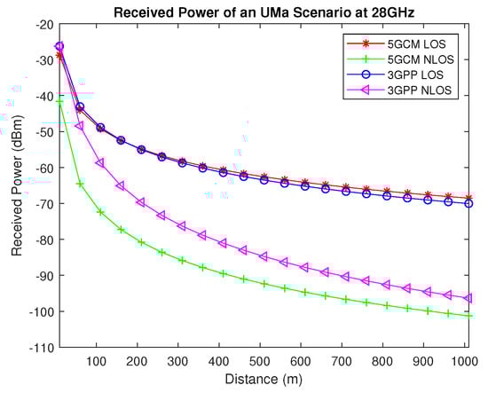
Figure 14. Received power of an Urban Macro environment at 28 GHz.

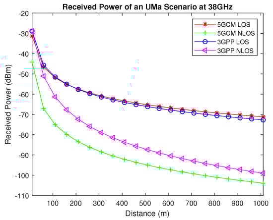
Figure 15. Received power of an Urban Macro environment at 38 GHz.

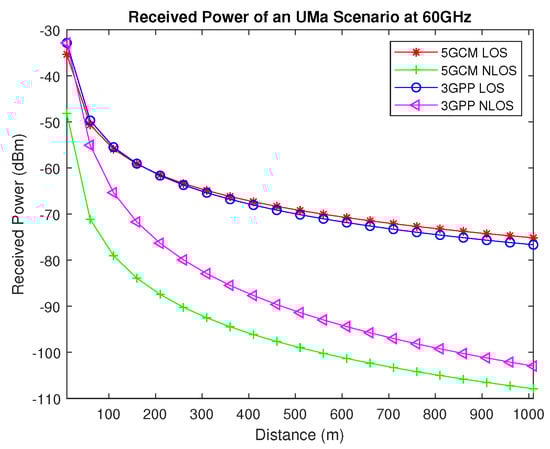
Figure 16. Received power of an Urban Macro environment at 60 GHz.

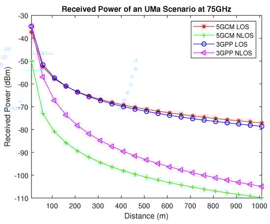
Figure 17. Received power of an Urban Macro environment at 75 GHz.

It can be seen from Figure 14, Figure 15, Figure 16 and Figure 17 that each model’s received power gradually reduces with distance and frequency. In comparison to the other models, the 5GCM and 3GPP model generates the highest signal power in LOS and NLOS scenarios, respectively. Table 5 displays the RP values for each model at various distances and frequencies.

Figure 18 measure and compare the RP of rural macro environment at 28 GHz, 38 GHz, 60 GHz, and 75 GHz. It can be seen from Figure 18 and Table 5 that received power gradually reduces with distance and frequency. received power in urban micro cells, urban and rural macro cells can be affected by various factors such as distance, obstacles, interference, base station antenna height, and frequency band. Observations from Figure 10, Figure 11, Figure 12, Figure 13, Figure 14, Figure 15, Figure 16, Figure 17 and Figure 18 show that the RP in urban micro cells is generally lower than in urban macro and rural macro cells due to the base station antenna height. The base station antenna height in urban and rural macro cells is generally higher than that of urban micro cells due to the difference in their coverage area and signal propagation characteristics.

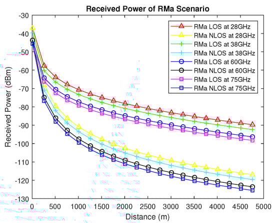
Figure 18. Received power of a Rural Macro environment.

This paper investigates various existing path-loss models for mmWave frequency bands to estimate path loss and received power. The results demonstrate that path loss and received power are influenced by factors such as operating frequency, the distance between transmitter and receiver antennas, antenna location, antenna height, and their respective positions. Among the models considered, the 5GCM model is found to minimize path loss and maximize receiver power specifically in the urban micro environment. On the other hand, the 3GPP model is suitable for both urban and rural macro environments, surpassing other models by producing the lowest path loss in those respective environments. These models are recognized as optimal choices for enhancing system performance in terms of path loss. Service providers can leverage these models to improve the quality of service in both indoor and outdoor 5G mmWave wireless networks.

5. Conclusions

Path loss and signal power in urban and rural environments can be affected by various factors such as distance, obstacles, interference, antenna height, and frequency band. The actual amount of loss will depend on the specific deployment and environmental factors. In this paper, mmWave frequency band, large-scale path-loss models and UMi, UMa, and RMa scenarios are considered to estimate the path loss and signal power. PL and RP are estimated for 28 GHz, 38 GHz, 60 GHz, and 75 GHz using various path-loss models. From the results, it is predicted that the path loss is lower and the signal power is higher in an urban micro scenario than the in urban macro and rural macro scenarios, and out of all four models used, the 5GCM model achieves lower path loss and higher signal power in all environments. In the future, we want to estimate and compare the path loss of urban micro, macro, and rural macro environments using optimization algorithms like GA, PSO, and GWO.

References

- Series, M. Guidelines for Evaluation of Radio Interface Technologies for IMT-2020; Report ITU 2512; 2017. Available online: https://www.itu.int/pub/R-REP-M.2412-2017 (accessed on 28 June 2023).
- William, L.; Queder, F.; Haucap, J. 5G: A new future for Mobile Network Operators, or not? Telecommun. Policy 2021, 45, 102086. [Google Scholar]
- Alquhali, A.H.; Roslee, M.; Alias, M.Y.; Mohamed, K.S. IOT Based Real-Time Vehicle Tracking System. In Proceedings of the 2019 IEEE Conference on Sustainable Utilization and Development in Engineering and Technologies (CSUDET), Penang, Malaysia, 7–9 November 2019; pp. 265–270. [Google Scholar]
- Billa, A.; Shayea, I.; Alhammadi, A.; Abdullah, Q.; Roslee, M. An overview of indoor localization technologies: Toward IoT navigation services. In Proceedings of the 2020 IEEE 5th International Symposium on Telecommunication Technologies (ISTT), Shah Alam, Malaysia, 9–11 November 2020; IEEE: Piscataway, NJ, USA, 2020; pp. 76–81. [Google Scholar]
- Kordi, K.A.; Alhammadi, A.; Roslee, M.; Alias, M.Y.; Abdullah, Q. A Review on Wireless Emerging IoT Indoor Localization. In Proceedings of the 2020 IEEE 5th International Symposium on Telecommunication Technologies (ISTT), Shah Alam, Malaysia, 9–11 November 2020; pp. 82–87. [Google Scholar]
- Rappaport, T.S.; Sun, S.; Mayzus, R.; Zhao, H.; Azar, Y.; Wang, K.; Wong, G.N.; Schulz, J.K.; Samimi, M.; Gutierrez, F. Millimeter wave mobile communications for 5G cellular: It will work! IEEE Access 2013, 1, 335–349. [Google Scholar] [CrossRef]
- Shu, S.; MacCartney, G.R.; Rappaport, T.S. A novel millimeter-wave channel simulator and applications for 5G wireless communications. In Proceedings of the 2017 IEEE International Conference on Communications (ICC), Paris, France, 21–25 May 2017; IEEE: Piscataway, NJ, USA, 2017. [Google Scholar]
- Mohamed, K.S.; Alias, M.Y.; Roslee, M.; Raji, Y.M. Towards green communication in 5G systems: Survey on beamforming concept. IET Commun. 2021, 15, 142–154. [Google Scholar] [CrossRef]
- Narekar, P.N.; Bhalerao, D.M. A survey on obstacles for 5G communication. In Proceedings of the 2015 International Conference on Communications and Signal Processing (ICCSP), Melmaruvathur, India, 2–4 April 2015; IEEE: Piscataway, NJ, USA, 2015. [Google Scholar]
- Imran, D.; Farooqi, M.M.; Khattak, M.I.; Ullah, Z.; Khan, M.I.; Khattak, M.A.; Dar, H. Millimeter wave microstrip patch antenna for 5G mobile communication. In Proceedings of the 2018 International Conference on Engineering and Emerging Technologies (ICEET), Lahore, Pakistan, 22–23 February 2018; IEEE: Piscataway, NJ, USA, 2018. [Google Scholar]
- Mardeni, R.; Subari, K.S.; Shahdan, I.S. Design of bow tie antenna in CST studio suite below 2GHz for ground penetrating radar applications. In Proceedings of the 2011 IEEE International RF & Microwave Conference, Seremban, Malaysia, 12–14 December 2011; IEEE: Piscataway, NJ, USA, 2011. [Google Scholar]
- Roslee, M.; Azmir, R.S.; Abdullah, R.; Shafr, H.Z.M. Road pavement density analysis using a new non-destructive ground penetrating radar system. Prog. Electromagn. Res. 2010, 21, 399–417. [Google Scholar] [CrossRef]
- Roy, S.; Tiang, R.J.J.; Roslee, M.B.; Ahmed, M.T.; Mahmud, M.P. Quad-band multiport rectenna for RF energy harvesting in ambient environment. IEEE Access 2021, 9, 77464–77481. [Google Scholar] [CrossRef]
- Osama, A.; Roslee, M.B.; Yusoff, Z.B. Simulated annealing for resource allocation in downlink NOMA systems in 5G networks. Appl. Sci. 2021, 11, 4592. [Google Scholar]
- Alquhali, A.H.; Roslee, M.B.; Alias, M.Y.; Mohamed, K.S. D2D communication for spectral efficiency improvement and interference reduction: A survey. Bull. Electr. Eng. Inform. 2020, 9, 1085–1094. [Google Scholar] [CrossRef]
- Docomo, N. White Paper on 5G Channel Model for Bands up to 100 GHz. Tech. Rep. 2016. Available online: http://www.5gworkshops.com/5gcm.html (accessed on 28 June 2023).
- Jaeckel, S.; Peter, M.; Sakaguchi, K.; Keusgen, W.; Medbo, J. 5G Channel Models in mm-Wave Frequency Bands. In Proceedings of the European Wireless 2016: 22th European Wireless Conference, Oulu, Finland, 18–20 May 2016; pp. 1–6. [Google Scholar]
- Medbø, J.I.; Borner, K.; Haneda, K.; Hovinen, V.; Imai, T.; Jarvelainen, J.; Jamsa, T.; Karttunen, A.; Kusume, K.; Kyrolainen, J.; et al. Channel modelling for the fifth generation mobile communications. In Proceedings of the 8th European Conference on Antennas and Propagation (EuCAP 2014), The Hague, Netherlands, 6–11 April 2014; IEEE: Piscataway, NJ, USA, 2014. [Google Scholar]
- Rappaport, T.S.; Xing, Y.; MacCartney, G.R.; Molisch, A.F.; Mellios, E.; Zhang, J. Overview of millimeter wave communications for fifth-generation (5G) wireless networks—With a focus on propagation models. IEEE Trans. Antennas Propag. 2017, 65, 6213–6230. [Google Scholar] [CrossRef]
- Oladimeji, T.T.; Kumar, P.; Oyie, N.O. Propagation path loss prediction modelling in enclosed environments for 5G networks: A review. Heliyon 2022, 8, E11581. [Google Scholar] [CrossRef]
- Oladimeji, T.T.; Kumar, P.; Elmezughi, M.K. Performance analysis of improved path loss models for millimeter-wave wireless network channels at 28 GHz and 38 GHz. PLoS ONE 2023, 18, e0283005. [Google Scholar] [CrossRef]
- Zhang, Y.; Wen, J.; Yang, G.; He, Z.; Wang, J. Path loss prediction based on machine learning: Principle, method, and data expansion. Appl. Sci. 2019, 9, 1908. [Google Scholar] [CrossRef]
- Jakob, T.; Zibar, D.; Christiansen, H.L. Model-aided deep learning method for path loss prediction in mobile communication systems at 2.6 GHz. IEEE Access 2020, 8, 7925–7936. [Google Scholar]
- Nguyen, C.; Cheema, A.A. A deep neural network-based multi-frequency path loss prediction model from 0.8 GHz to 70 GHz. Sensors 2021, 21, 5100. [Google Scholar] [CrossRef] [PubMed]
- Hasan, R.; Mowla, M.M.; Rashid, M.A.; Hosain, M.K.; Ahmad, I. A statistical analysis of channel modeling for 5G mmwave communications. In Proceedings of the 2019 International Conference on Electrical, Computer and Communication Engineering (ECCE), Cox’s Bazar, Bangladesh, 7–9 February 2019; IEEE: Piscataway, NJ, USA, 2019. [Google Scholar]
- Lodro, M.; Majeed, N.; Khuwaja, A.A.; Sodhro, A.H.; Greedy, S. Statistical channel modelling of 5G mmWave MIMO wireless communication. In Proceedings of the 2018 International Conference on Computing, Mathematics and Engineering Technologies (iCoMET), Sukkur, Pakistan, 3–4 March 2018; IEEE: Piscataway, NJ, USA, 2018. [Google Scholar]
- Aldhaibani, A.O.; Rahman, T.A.; Alwarafy, A. Radio-propagation measurements and modeling in indoor stairwells at millimeter-wave bands. Phys. Commun. 2020, 38, 100955. [Google Scholar] [CrossRef]
- Brata, M.; Zakia, I. Path Loss Estimation of 5G Millimeter Wave Propagation Channel—Literature Survey. In Proceedings of the 2021 7th International Conference on Wireless and Telematics (ICWT), Yogyakarta, Indonesia, 21–22 July 2022; IEEE: Piscataway, NJ, USA, 2021. [Google Scholar]
- MacCartney, G.R.; Zhang, J.; Nie, S.; Rappaport, T.T. Path loss models for 5G millimeter wave propagation channels in urban microcells. In Proceedings of the 2013 IEEE Global Communications Conference (GLOBECOM), Atlanta, GA, USA, 9–13 December 2013; IEEE: Piscataway, NJ, USA, 2013. [Google Scholar]
- Abhayawardhana, V.S.; Wassell, I.J.; Crosby, D.B.; Sellars, M.P.; Brown, M. Comparison of empirical propagation path loss models for fixed wireless access systems. In Proceedings of the 2005 IEEE 61st Vehicular Technology Conference, Stockholm, Sweden, 30 May–1 June 2005; IEEE: Piscataway, NJ, USA, 2005; Volume 1. [Google Scholar]
- Roslee, B.M.; Kwan, K.F. Optimization of Hata propagation prediction model in suburban area in Malaysia. Prog. Electromagn. Res. C 2010, 13, 91–106. [Google Scholar] [CrossRef]
- Obot, A.; Simeon, O.; Afolayan, J. Comparative analysis of path loss prediction models for urban macrocellular environments. Niger. J. Technol. 2011, 30, 50–59. [Google Scholar]
- Masui, H.; Kobayashi, T.; Akaike, M. Microwave path-loss modeling in urban line-of-sight environments. IEEE J. Sel. Areas Commun. 2002, 20, 1151–1155. [Google Scholar] [CrossRef]
- Xue, Q.; Liu, Y.; Sun, Y.; Wang, J.; Yan, L.; Feng, G.; Ma, S. Beam Management in Ultra-Dense mmWave Network via Federated Reinforcement Learning: An Intelligent and Secure Approach. IEEE Trans. Cogn. Commun. Netw. 2023, 9, 185–197. [Google Scholar] [CrossRef]
- Lin, Z.; Lin, M.; Champagne, B.; Zhu, W.; Al-Dhahir, N. Secrecy-Energy Efficient Hybrid Beamforming for Satellite-Terrestrial Integrated Networks. IEEE Trans. Commun. 2021, 69, 6345–6360. [Google Scholar] [CrossRef]
- Lin, Z.; An, K.; Niu, H.; Hu, Y.; Chatzinotas, S.; Zheng, G.; Wang, J. SLNR-Based Secure Energy Efficient Beamforming in Multibeam Satellite Systems. IEEE Trans. Aerosp. Electron. Syst. 2023, 59, 2085–2088. [Google Scholar] [CrossRef]
- Lin, Z.; Niu, H.; An, K.; Wang, Y.; Zheng, G.; Chatzinotas, S.; Hu, Y. Refracting RIS-Aided Hybrid Satellite-Terrestrial Relay Networks: Joint Beamforming Design and Optimization. IEEE Trans. Aerosp. Electron. Syst. 2022, 58, 3717–3724. [Google Scholar] [CrossRef]
- Rappaport, T.S.; MacCartney, G.R.; Samimi, M.; Sun, S. Wideband millimeter-wave propagation measurements and channel models for future wireless communication system design. IEEE Trans. Commun. 2015, 63, 3029–3056. [Google Scholar] [CrossRef]
- MacCartney, G.R., Jr.; Sun, S.; Rappaport, T.T.; Xing, Y.; Yan, H.; Koka, J.; Wang, R.; Yu, D. Millimeter wave wireless communications: New results for rural connectivity. In Proceedings of the 5th Workshop on all Things Cellular: Operations, Applications and Challenges, New York, NY, USA, 3–7 October 2016. [Google Scholar]
- Thomas, T.A.; Rybakowski, M.; Sun, S.; Rappaport, T.T.; Nguyen, H.C.; Kovács, I.Z.; Rodriguez, I. A prediction study of path loss models from 2 to 73.5 GHz in an urban-macro environment. In Proceedings of the 2016 IEEE 83rd Vehicular Technology Conference (VTC Spring), Nanjing, China, 15–18 May 2016; IEEE: Piscataway, NJ, USA, 2016. [Google Scholar]
- Haneda, K.; Tian, L.; Zheng, Y.; Asplund, H.; Li, J.; Wang, Y.; Steer, D.; Li, C.; Balercia, T.; Lee, S.; et al. 5G 3GPP-like channel models for outdoor urban microcellular and macrocellular environments. In Proceedings of the 2016 IEEE 83rd Vehicular Technology Conference (VTC Spring), Nanjing, China, 15–18 May 2016; IEEE: Piscataway, NJ, USA, 2016. [Google Scholar]
- Sun, S.; Thomas, T.A.; Rappaport, T.T.; Nguyen, H.C.; Kovács, I.Z.; Rodriguez, I. Path loss, shadow fading, and line-of-sight probability models for 5G urban macro-cellular scenarios. In Proceedings of the 2015 IEEE Globecom Workshops (GC Wkshps), San Diego, CA, USA, 6–10 December 2015; IEEE: Piscataway, NJ, USA, 2015. [Google Scholar]
- Rappaport, T.S.; Sun, S.; Shafi, M. Investigation and comparison of 3GPP and NYUSIM channel models for 5G wireless communications. In Proceedings of the 2017 IEEE 86th Vehicular Technology Conference (VTC-Fall), Toronto, ON, Canada, 24–27 September 2017; IEEE: Piscataway, NJ, USA, 2017. [Google Scholar]
- MacCartney, R.G.; Rappaport, T.S. Rural macrocell path loss models for millimeter wave wireless communications. IEEE J. Sel. Areas Commun. 2017, 35, 1663–1677. [Google Scholar] [CrossRef]
- Bernard, S. Digital Communications; Prentice Hall: Upper Saddle River, NJ, USA, 2001; Volume 2. [Google Scholar]
Disclaimer/Publisher’s Note: The statements, opinions and data contained in all publications are solely those of the individual author(s) and contributor(s) and not of MDPI and/or the editor(s). MDPI and/or the editor(s) disclaim responsibility for any injury to people or property resulting from any ideas, methods, instructions or products referred to in the content. |
© 2023 by the authors. Licensee MDPI, Basel, Switzerland. This article is an open access article distributed under the terms and conditions of the Creative Commons Attribution (CC BY) license (https://creativecommons.org/licenses/by/4.0/).