Experimental Investigation on Heat Transfer Characteristics of Liquid Nitrogen Spray Cooling for Large Area

Abstract

Spray cooling has demonstrated advantages in the thermal control of avionic devices. In this study, a spray cooling system is established using liquid nitrogen (LN2) as a working fluid to investigate the effect of heat transfer characteristics on a large heating surface. The temperature response measurement and experimental analysis of the heating surface of a large-area shell structure under the boundary conditions of different heat flux and temperature regions were carried out. The temperature response curves for the outer surface of the shell structure from the initial temperature to the set temperature were obtained under different heat flows and temperature zones. The results show that the thermal response time of the surface spray phase cooling is less than 2 s, the stability time for the cooling temperature of the covering layer is longer than 60 s, and the cooling state can be maintained for 30 min under different working conditions. This study can provide a technical reference for the application of spray systems in the field of aircraft cooling.

1. Introduction

In contrast to simple wall heat transfer, the spray cooling process refers the heat transfer between the multi-phase fluid and the solid wall with numerous heat transfer parameters, so the heat transfer mechanism is relatively complex. As the current models used in numerical simulations are generally based on certain assumptions, it is difficult to describe the process of spray heat transfer through simple simulation analysis completely and accurately [1,2,3]. Therefore, experimental research becomes the main method to study spray cooling. While the actual spray heat transfer process is reproduced, the corresponding phenomenon is observed and the heat transfer rule of spray cooling is summarized [3,4].

An important characteristic of spray cooling is the ability to prevent liquid from separating from the surface during intense boiling. The momentum of the droplet enables the liquid to penetrate the vapor barrier formed by the nucleation of the bubble and to replenish the surface more effectively, which is of great benefit to high-density cooling [5].

However, spray cooling also has its drawbacks; chief among them is that sometimes the high-pressure drops are required to atomize liquid flows into tiny droplets. Moreover, the narrow flow passage inside the nozzle increases the possibility of clogging, which may cause the surface to eventually burn out. Moreover, even small changes in the manufacturing of seemingly identical nozzles can make a huge difference in the spray [6,7,8,9]. Therefore, it is necessary to perform careful predictive tests of nozzles to ensure the cooling performance is predictable and repeatable [10]. Despite these disadvantages, spray cooling is still very popular in both low- and high-temperature applications. It is worth mentioning that the spray cooling device also exists in the refrigeration system, in which the spray chamber serves as the evaporator of the refrigeration loop [11,12].

Spray cooling is characterized by its strong heat exchange ability, small temperature difference during cooling, high-temperature uniformity, and low demand for a working medium [13,14,15,16]. There are several heat transfer mechanisms in the spray cooling process, such as droplet evaporation, droplet impact on the wall, liquid film evaporation, forced convection, surface nucleation boiling, and secondary nucleation. The first two are the initial stages, which are also the stages of heat flux from low to high. The heat flux of heat transfer rapidly rises with the droplet from the nozzle to the wall to form a stable liquid film, and then begins to decline to a level that is still relatively high compared with other heat transfer methods. Liquid film evaporation and forced convection are the main heat transfer mechanisms throughout spray cooling. The last two exist in the two-phase heat transfer zone, where the fluid flow situation is relatively complex.

Guo [17] studied the single-hole oil syringe with the pressure of the spray chamber and the inlet temperature as variables. Lin [16] took the closed spray cooling system with the working medium of R410A as the research object to optimize the height of spray and the aperture of nozzle. Zhao X [14] took the circulating spray cooling system with the working medium of water as the research object to analyse the relationship between the heat flux, liquid subcooling degree, distance between the nozzle and wall surface, injection pressure of the nozzle, spray volume flow rate, and droplet diameter distribution. Taking the closed flash spray cooling system with the working medium of R1336mzz as the research object, Zhang [15] experimentally studied the effects of spray flow rate, inlet temperature (which can be described as superheat), and spray chamber pressure on heat transfer performance, which showed that the fluid parameters affecting the heat flux and temperature distribution uniformity of spray cooling mainly include inlet pressure, spray chamber pressure, flow rate, spray height, wall superheat, and so on.

The position between the nozzle and the wall surface will affect the heat transfer performance of spray cooling. Silk [18] took a closed cycle spray cooling system with the working medium of PF-5060 as the research object, which showed that the surface heat transfer ability of the non-vertical wall spray in the two-phase zone was significantly improved compared with the vertical wall spray by changing the angle between the spray axis of the nozzles at the same height and the normal direction of the wall between 0° and 45°. Liu [19] took the closed circulation spray cooling system with the working medium of surfactant water as the research object, while the tilt angle was 18°. Lily [20] took the water working medium open-cycle spray cooling steel plate as the research object and made it clear that it was in a two-phase region, which suggested that there was an optimal spray angle significantly reducing the boiling effect of spray cooling film. Taking the water circulation spray cooling system as the research object, Zhao [21] analysed the influence of different parameters of the downward, upward, left, and vertical spray nozzle on the heat flux. The results show that there is no significant difference in each area of spray cooling. The results obtained in the above experiments were different. Some researchers thought there was an optimal spray angle, while others believed that vertical spray had the best effect. In general, however, the spray angle had little impact on the heat transfer performance of the system. The reason is that although the increase of the inclination angle reduced the impact area, a larger inclination angle, on the contrary, enabled the spray drops to pass over the heat source more quickly. In this case, the convective heat transfer became stronger so that the total heat transfer performance of the system remained almost constant [22].

With the increasing research on spray cooling, the study of the smooth surface has become more sufficient. Studies show that the structure of the heat exchange surface has a great influence on the heat flux of spray cooling. Hsieh, C.C. [23] used high-speed photography to visualize heat transfer on the surface of the microgroove. Based on the observed phenomena and the experimental heat flux curve, the heat transfer process is divided. Silk [18] used the pF-5060 working medium and a micro-structure of different shapes and sizes spray system as the research object. Under the condition of fixed flow rate and nozzle height, it was found that the micro-structure significantly enhanced the heat transfer performance of spray cooling. Silk’s experimental results are consistent with the literature [24], which indicates that the heat transfer capacity of surfaces with straight ribs, square ribs, triangular ribs, and smooth surface decreases in turn. Salman [25] used a closed spray cooling system with a deionized water working medium as the research object and designed three kinds of grooves for the experimental study in a non-boiling area under the different backpressures of a spray chamber. Liu [24] used a closed-cycle spray cooling system with working medium water as the research object and designed three kinds of grooves. Combined with the tilted spray, the groove was designed linearly. The varying distances at the top and bottom of the groove make the section appear as a rectangle, a trapezoid, and a triangle. At present, spray cooling technology can be used in many industries and fields, such as cryogenic wind tunnels, aerospace, and the refrigeration medical and electronic industry. In recent years, the team at Xi’an Jiaotong University has carried out research on liquid nitrogen spray cooling technology related to low temperature wind tunnels, and has achieved certain results. However, the research results of liquid nitrogen spray cooling technology applied to surface heat transfer characteristics are less at home and abroad [26]. Therefore, this research will study the mechanism of a large area cryogenic spray cooling system with liquid nitrogen as the working fluid, including the impact of several full-cone sprays on a heated, lightweight, thin shell structure. Experimentally measured data is obtained and corresponding empirical curves are plotted and analysed. The results and discussion of the experiment will provide support for the subsequent thermal control technology innovation, which covers large areas, has a fast response time, and long-term stability.

2. Experimental Set-Up

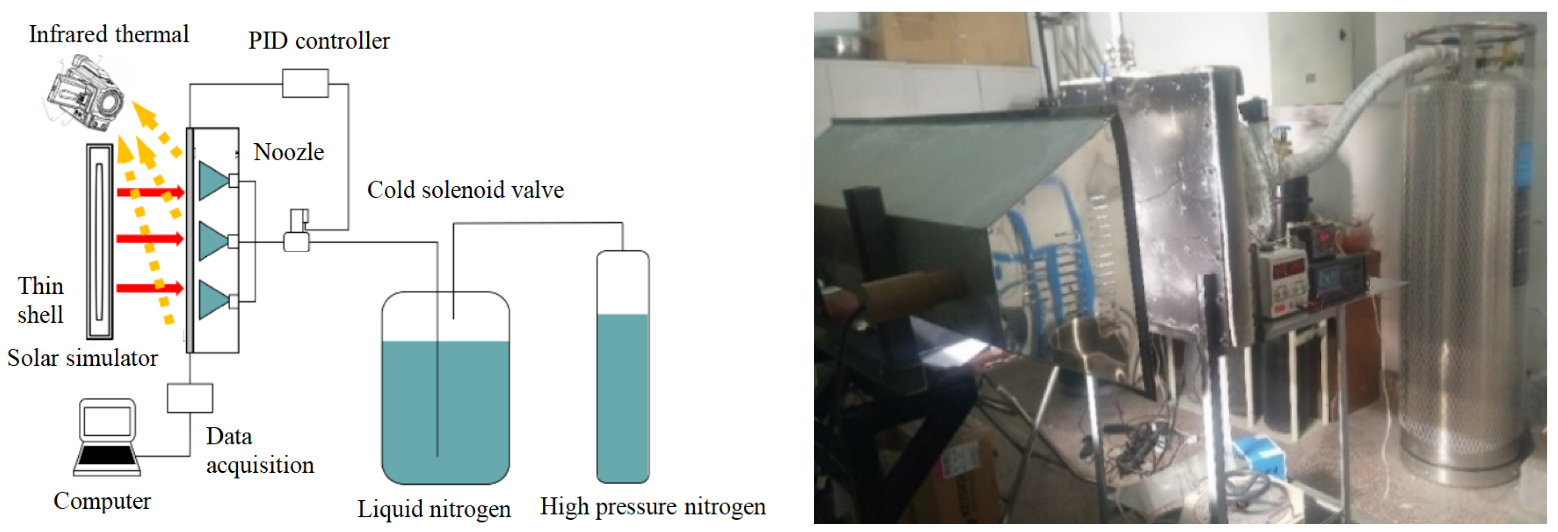
The experimental bench is mainly composed of the heating system, a liquid supplying system, and a measuring system. The liquid supply system includes nozzles, coolant, a liquid storage tank, and a solenoid valve. The heating system includes quartz heating lamps and electric heating sheets. The measurement system includes a thermocouple, a data acquisition instrument Keysight DAQ970A, an infrared thermal imager, and a thermal flowmeter. The schematic diagram of the large-area spray cooling experimental bench is shown in Figure 1 and Figure 2.

2.1. Spray System

As indicated in the literature [27], more nozzles lead to a higher heat flux density and better heat flux on the heat surface. Considering more difficulties and costs brought by the increase of nozzles during manufacture, there should be a proper nozzle number in a certain space. The test case is performed by a commercial CFD software a commerical CFD software to verify the appropriateness of the nozzle array.

Spray cooling is a complex multiphase flow system composed of a discrete phase and a continuous phase. In the spray cooling simulation, we turn on the discrete phase model to track and calculate the momentum, mass, and temperature changes of nitrogen droplets in the heat transfer process.

Considering the influence of gravity and resistance in the movement, the force balance equation of droplet is

$$\frac{\mathrm{d}{u}_d}{\mathrm{d}t}=F_D(u_a-u_d)+\frac{g({\rho }_d-{\rho }_a)}{{\rho }_d}$$

(1)

where, subscript D indicates that the parameter is the relevant value of the droplet, and F_D is defined as $F_D=\frac{18\mu }{{\rho }_d{d}_d^2}\frac{C_D{\mathrm{Re}}_d}{24}$, $C_D=a_1+\frac{a_2}{\mathrm{Re}}+\frac{a_3}{{\mathrm{Re}}^2}$, ${\mathrm{Re}}_d=\frac{{\rho }_a{d}_d\left|u_d-u_a\right|}{\mu }$.

In [27], $C_D$ in the above formula can be also calculated by the following equation, that is $C_D=\frac{24}{\mathrm{Re}}(1+0.186{\mathrm{Re}}^{0.6526})+\frac{0.44\mathrm{Re}}{7185.3535 + \mathrm{Re}}$. By comparing the two related equations, we can find $a_1$, $a_2$ and $a_3$, the specific calculation formula will not be repeated here.

Considering the convection and evaporation of each droplet, the heat balance equation is

$$m_d{c}_p\frac{\mathrm{d}{T}_d}{\mathrm{d}t}=h_c{A}_d(T_a-T_d)-\frac{\mathrm{d}{m}_d}{\mathrm{d}t}{L}_h$$

(2)

where, h_c is related to specific heat transfer conditions which is different from h below.

The mathematical description of droplet evaporation can refer to [27]. After simplifying the relevant equations, the mass conservation equation can be further derived, that is

$$\mathrm{div}({\rho }_d{u}_d)=\frac{\mathrm{d}{m}_d}{\mathrm{d}t}$$

(3)

The nozzle is designed, as shown in

Table 1. Characteristics of spray nozzle in test case.

Nozzle Type	Orifice Diameter (mm)	Spray Angle (°)	Distance to Heat Surface (mm)	Flow Rate (kg/s)
Cone	1.6	120	42	0.022832933

. The size of the test specimen is 570 mm × 570 mm × 3 mm. Considering the installation, the effective cooling area is designed as 500 mm × 500 mm. When the heat flux of the thin shell surface is 16,000 W/m², the whole process takes 30 s. Spray cooling of the test surface begins at the 8th second. The temperature of the test surface with three different grid arrangements (3.53 × 10⁵, 1.72 × 10⁶, and 2.67 × 10⁶ nodes) is examined. According to the refinement of the subsequent simulation results, the grid arrangement of 1.72 × 10⁶ and 2.67 × 10⁶ has a better performance than that of 3.53 × 10⁵. Thus, a grid size of 1.72 × 10⁶ is selected in all subsequent simulations.

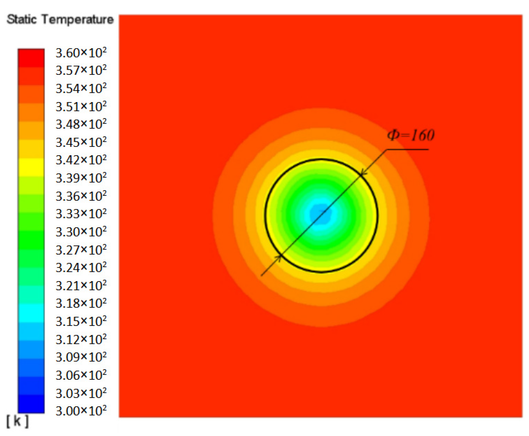
Figure 3 shows the steady-state temperature distribution of the test surface for a single nozzle. A single nozzle would cause uneven temperature distribution on the test surface and could not meet the requirements of large-area cooling.

The numerical simulation result shows that the effective cooling area of a single nozzle is an approximate circle with a radius of 80 mm. Considering more difficulties and costs brought about by the increase of nozzles during manufacture, and using the spray as efficiently as possible, the space of 166.667 mm is taken to cover all the cooling area of 500 mm × 500 mm, which means nine nozzles will be evenly distributed in both vertical and horizontal directions, as shown in Figure 4.

In the spray system, nine stainless steel micro-liquid nozzles with the outlet aperture of 1.6 mm and the spray cone angle of about 120 degrees are used. The distance between the nozzle and the surface is 42 mm. The flow rate is directly proportional to the square root of the pressure difference. More specific relationships are shown in

Table 2. Relationship between nozzle flow and pressure difference.

the Pressure Difference (bar)	0.7	1	1.5	2	3	4	6
Flow Rate (L/min)	1.1	1.3	1.5	1.7	2.1	2.4	2.9

.

A thin aluminium shell is used as the object of the experiment, while the relative position between the nozzles and the aluminium plate is shown in Figure 4. The nozzles are evenly distributed on the fixed plate and the size of the spray cooling area is 500 × 500 mm. Liquid nitrogen is used as the working medium for the liquid supply system.

2.2. Heater Assembly

The heating system has two modes. When the heat flux on the shell surface is low, non-contact radiation heating of quartz lamps is adopted based on the measurement demand of infrared radiation imaging. The maximum thermal power is 1367 W/m². When the heat flux on the shell surface is high, electric heating sheets are used for heating in the experiment. The maximum heating power is 4 kW, and the heating power per unit area is within 0.01~2 W/cm². The working temperature should be lower than 180 °C. On one side, there is a rubber layer that can be in close contact with the heated object. And on the other side is a 10 mm-thick insulation layer with low-emissivity tin foil on the surface, which can reduce the influence of the environment on the temperature of the heating sheet.

2.3. Experimental Measurement Facilities

Considering the measurement under low-temperature condition and the thermal contact resistance on the surface of the aluminium plate, the T-type thermocouple with a small diameter produced by the Omega company, named TT-T-36-SLE, is selected. The arrangement of 20 thermocouples is shown in Figure 5.

The red circle represents the central point of the nozzle, the blue circle represents the diagonal intersection area of the nozzle, the green circle represents the horizontal intersection area and vertical intersection area of the nozzle, and the yellow circle represents the upper and lower interfaces.

The temperature signals of all thermocouples are collected by the Keysight DAQ970A data acquisition instrument and then transmitted to the computer for real-time monitoring and analysis. In addition, the FLIR T600 infrared thermal imager and HFM-201 radiant heat flowmeter are used in this experiment.

3. Heat Loss and Experimental Errors

3.1. Heat Loss

To reduce the heat leakage of the liquid nitrogen spray cooling system as far as possible and thus reduce the heat loss of liquid nitrogen, it is necessary to conduct an adiabatic design for the low-temperature loop system. Considering the cost of the experiment, accumulating insulation is suitable for complex adiabatic space as it doesn’t need to work in a vacuum environment. Therefore, this adiabatic method is chosen.

The rubber-coated polystyrene foam with thermal conductivity of 0.42 W/(m·K) is used in the experiment for thermal insulation. The thickness of the accumulated adiabatic layer has a considerable influence on the heat leakage and the temperature rise of the system. The limit method and the single-layer cylindrical wall heat transfer formula are used to obtain the related calculation to 1/2 inch of the wall. The curve of heat leakage with the thickness of the insulation layer is shown in Figure 6. According to the results, a 30 mm-thick insulation material is selected to wrap the whole loop.

3.2. Experimental Errors

There are mainly two kinds of experimental errors. One is the environmental error caused by the non-ideal thermal environment around the experimental system, and the other is the error caused by the limitation of the instrument precision regarding the measurements.

The main influence of the thermal environment of the system on the experimental conditions is that the ambient temperature has a heating effect, not only on the experimental heating surface but also on the fluid in the pipeline. Although insulation measures have been taken for the experimental and piping systems, the heat transfer from the environment to the pipeline is relatively smaller compared to the electric heating and spray cooling processes, and the heat transfer between the thermal components and their supporting parts cannot be ignored. As time goes on, the surface temperature of the support component in contact with the thermal component will gradually decrease to as low as 11.6 °C. Therefore, the heat conduction loss between the thermal component and its support component will lead to a calculation error in the heat transfer coefficient of spray cooling convection.

Secondly, during inefficient phase-change spray cooling experiments, there is no closure space around the heated plate in the process of quartz lamp heating under the assumption that the temperature of the other four sides, except the heating surface of the quartz lamp, is 292.15 K and the angle coefficient is 0.2. When the temperature of the heating surface drops to −40 °C, the heat exchange between the environment and the heated wall surface reaches 800 W, and the heat flux reaches 3200 W/m². Therefore, the actual heat flux on the surface will be greater than the measured heat flux of the quartz lamps when we consider heating in this way. However, it does not affect its temperature response index, which can be achieved at a larger heat flux, and the temperature response can also be achieved at a smaller heat flux.

Lastly, during the heating process of the electrical heating film, although there is an insulating layer set up on the outer surface of the electrical heating sheet, there is still a heat exchange in the insulation layer, and the loss of the heat flux is generally 200~300 W/m², accounting for 2–3% of the total heat flux.

3.3. Instruments Errors

The principle of thermocouples is contact temperature measurement, which makes the temperature-measuring element reach thermal equilibrium with the measured object. In actual engineering, the temperature of the measured object changes quickly, and the temperature-measuring element does not reach the equilibrium state, so the response time of the thermocouple has a great influence on the accuracy of the transient temperature measurement. It is necessary to pay attention to the diameter of the thermocouple wire and the degree of vulnerability to make a choice. The smaller the diameter of the thermocouple wire, the shorter the response time. The response error can be obtained by Equation (4)

$$\Delta \theta =\Delta {\theta }_0{\mathrm{e}}^{-t/\tau }$$

(4)

where $\Delta \theta$ is the error caused by the measuring element at time t, and $\Delta {\theta }_0$ is the error caused by the measuring element at the initial moment.

In unit time, the radiation heat transfer capacity of the quartz lamp and thermocouple can be expressed as Equation (5)

$$E=\sigma \epsilon \mathrm{A}(T_s^4-T_{tc}^4)$$

(5)

where A is the surface area of the wall.

In unit time, the heat of the thermocouple convection with the surrounding gas and heat conduction exchange with the test plate is

$$Q=\mathrm{hA}(T-T_{tc})-\frac{T_w-T_{tc}}{\mathrm{R}}$$

(6)

where R is the thermal resistance between the thermocouple and the wall.

In the steady state, $E=Q$, and the influence of thermal radiation on thermocouple temperature measurement error is

$$T_{tc}-T_w=(\sigma \epsilon \mathrm{A}(T_s^4-T_{tc}^4)-\mathrm{hA}(T-T_{tc}\left)\right)\times \mathrm{R}$$

(7)

where T_w is the wall temperature, h is the convective heat transfer coefficient between the thermocouple and the surrounding gas, and T is the ambient gas temperature.

According to the above formulas, under the measured temperature in the range of −40 °C~+30 °C, the absolute measurement error caused by thermal radiation and contact thermal resistance is around 0.55 °C, and the relative measurement error is +0.18%~+0.23%. The accuracy and range of the instruments and measuring equipment selected in the experiment are shown in

Table 3. Parameters of experimental instruments.

The Name of the Instrument	Scale Range	Error Range
TT-T-36-SLE thermocouple	−200 °C–260 °C	±0.4%
Infrared thermal imager	7.5–14 μm	±2%
Data acquisition instrument (Keysight DAQ970A)	—	0.004%

.

In the experiment, a FLIR T600 infrared thermal imager with a measuring wavelength of 7.5~14 µm, a temperature range of −40 °C~650 °C, and a thermal sensitivity of less than 0.04 °C at 30 °C is used. The factors that affect the temperature measurement accuracy of infrared thermography include the emissivity of the object itself, ambient temperature, measurement distance, humidity, etc. The experimental measurement results show that the measurement error is 0.7~0.9 K in the short-wave working band under the emissivity deviation of 0.1 for the high-emissivity material. In actual measurements, frost will appear on the surface of the thermal component due to the decrease of temperature, so the main error is the temperature measurement error caused by the change of emissivity of the measured surface. To ensure the data accuracy of infrared thermography at deep-low temperatures, black paint is evenly applied to the temperature-measured surface in the experiment, and then the emissivity of the coated surface is corrected by the temperature of the thermocouple so that we can obtain the real temperature distribution field. In addition, the temperature measurement accuracy will be further improved by adjusting the position of the thermal imager.

4. Results and Discussion

4.1. Effect of Injection Pressure/Flow Rate on Cooling

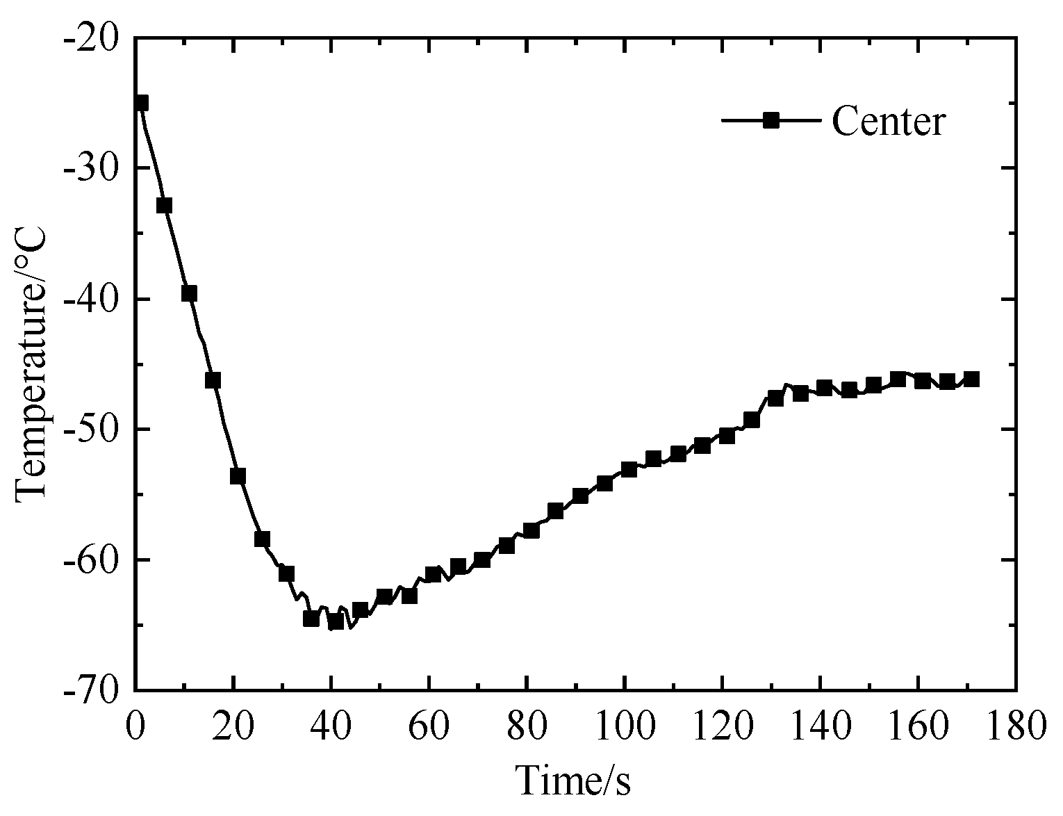
Adjust the pressure-reducing valve on the nitrogen tank to reach a driving pressure of 0.4 MPa and 0.2 MPa, respectively. The temperature response curve under the driving pressure of 0.4 MPa without heating is shown in Figure 7. The Stable temperature set by the PID controller is −40 °C. As shown, the temperature fell from −25 °C to −40 °C within 10 s. However, due to the high drive pressure loop of liquid nitrogen flow, the current research shows that the relationship between flow rate and heat transfer is positively correlated. Therefore, the PID proportion coefficient is very large. Moreover, the Integral and differential coefficient has too much overshoot, while the electromagnetic valve closed until −65.3 °C and then began to rebound. The heating power of the environment on light, thin shell structure parts is small, so the temperature raised slowly with a long oscillation period.

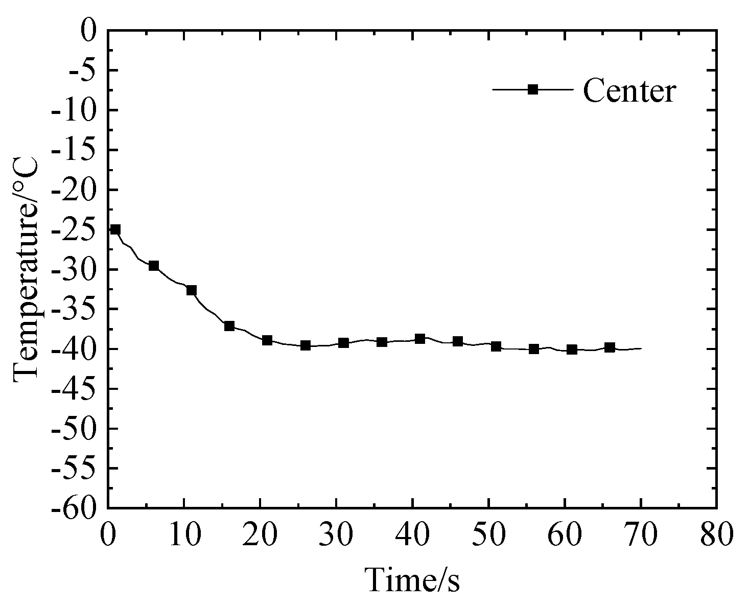
Although under 0.4 MPa, the response time conforms to the designed requirements, in the open and close process of the solenoid valve, the pressure fluctuation is large, and the pipe joint will produce a large load. Moreover, the temperature overshoot is large, and the temperature recovery of the aluminium plate surface is slow. The dichotomy is adapted to select an appropriate driving pressure. The temperature response curve under the driving pressure of 0.2 MPa is shown in Figure 8. The stable temperature set by the PID controller is −40 °C. As shown, the temperature at the centre of the heated surface fell from −25 °C to −40 °C in 30 s, the average temperature after stabilization is −39.57 °C, and the deviation is +0.4%/−0.3%. The result shows that temperature control under this condition is of a better effect and has less overshoot, the response time conducts to the requirements, and the bearing capacity requirements to the pipeline decreases.

The experimental data of the temperature at the center point are shown in

Table 4. Experimental data of three-stage central point temperature without heating and at 0.2 Mpa.

	Initial Temperature (°C)		Response Time (s)	Time Required for Stabilization (s)	Stable Temperature (°C)
	Average	Deviation			Average	Deviation
The center	−25	±0.6%	<2	30	−39.6	±0.4%

.

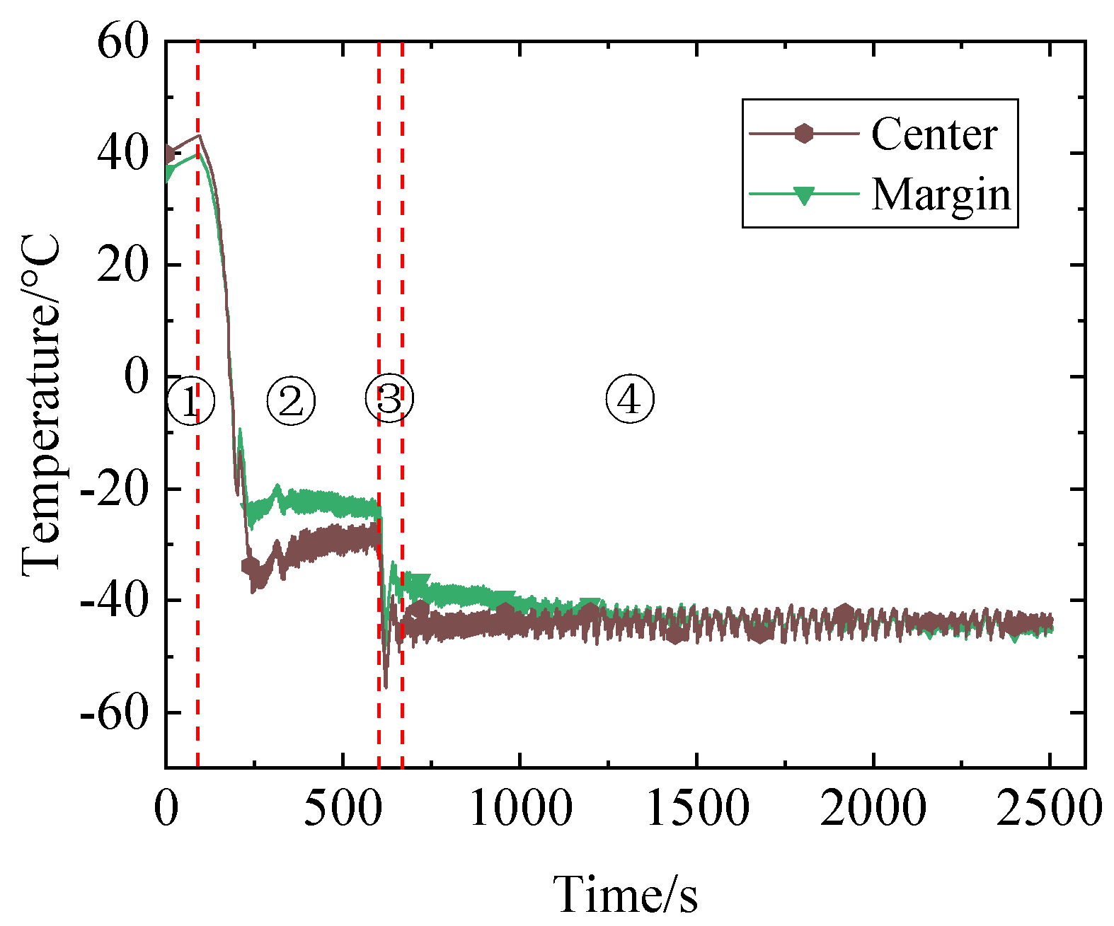
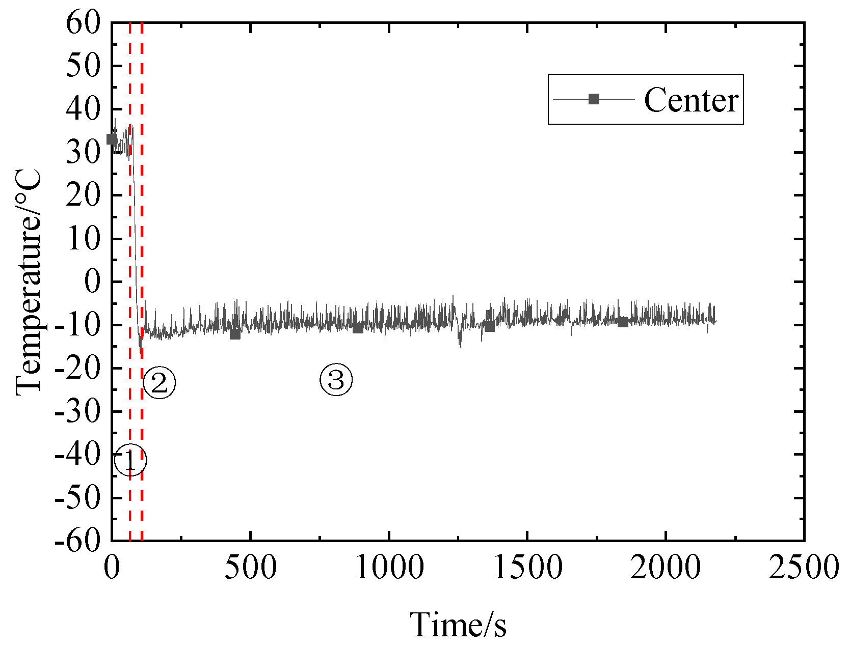
4.2. Spray Cooling Experiment under Low Heat Flux Condition

Set the heat flux of working condition 1 as 400 W/m². The heating surface temperature of the thin shell was reduced from −25 °C to −40 °C, and the experimental curves at 0.2 Mpa and 400 W/m² are shown in Figure 9, which is divided into four stages: ① initial thermal boundary, ② simulated thermal boundary, ③ rapid response, and ④ continuous stability.

(1)

Initial stage

In the initial stage, the function is to adjust the position of the quartz array lamp, measure the heat flux on the surface of the aluminum plate, and evaluate the heating uniformity. The rise of the aluminium plate’s temperature is the inevitable result of this series of operations.

(2)

Thermal boundary simulation

The wall temperature in the first rapid descent stage was 248 K. As the actual heat flux increases when the temperature of the surface drops, the regulation of the variable heat flux cannot be realized temporarily. Therefore, the limit method was adopted by directly taking the required theoretical value of the temperature after cooling as the basis when calculating the heat flux of heating. If the technical index can be completed well under this heat flux, they can also be experimentally achieved sufficiently under the condition that the wall temperature gradually decreases and the heat flux gradually increases to the heat flux set in the experiment.

(3)

Rapid response phase

The third stage is the rapid response stage, in which the temperature will be quickly reduced to the required temperature and achieve stability. Under the experimental conditions of 400 W/m² and 0.2 MPa, the response time is shorter than 2 s, and the time required for stability is 28 s. Calculate the average temperature every 20 s after the measured value reaches the set temperature for the second time. If the temperature difference of the average temperature is within 1 °C, the experiment has reached stability.

(4)

Stability stage

The fourth stage is the continuous stability stage with a stability time of 30 min. The specific parameters are shown in

Table 5. Experimental data of three stages under the heat flux of 400 W/m².

	Initial Temperature (°C)		Response Time (s)	Time Required for Stabilization (s)	Stable Temperature (°C)
	Average	Upper/Lower Limit			Average	Upper/Lower Limit
Center	−28.6	+0.9%/−1.4%	<2	28	−43.7	+2%/−2%
Peripheral central point	−22.7	+0.9%/−1.5%	<2	28	−42.6	+4%/−2%

. The average temperature of the central temperature measuring point and the peripheral central temperature measuring point are −43.7 °C and −42.6 °C, respectively, and the upper and lower limits are +2%/−2% and +4%/−2%, respectively. The unit of temperature in the table is °C. The average value is the average of the measurement points in the space, and the upper and lower limits are the ratio of the difference between the average value and the maximum deviation point of the average value of the contrast temperature in the space. From the absolute deviation, the temperature fluctuation of the single point after stabilization is ±4.5 °C. The reason for the fluctuation is that the solenoid valve only has the on–off function and cannot obtain the constant flow required when it is stable.

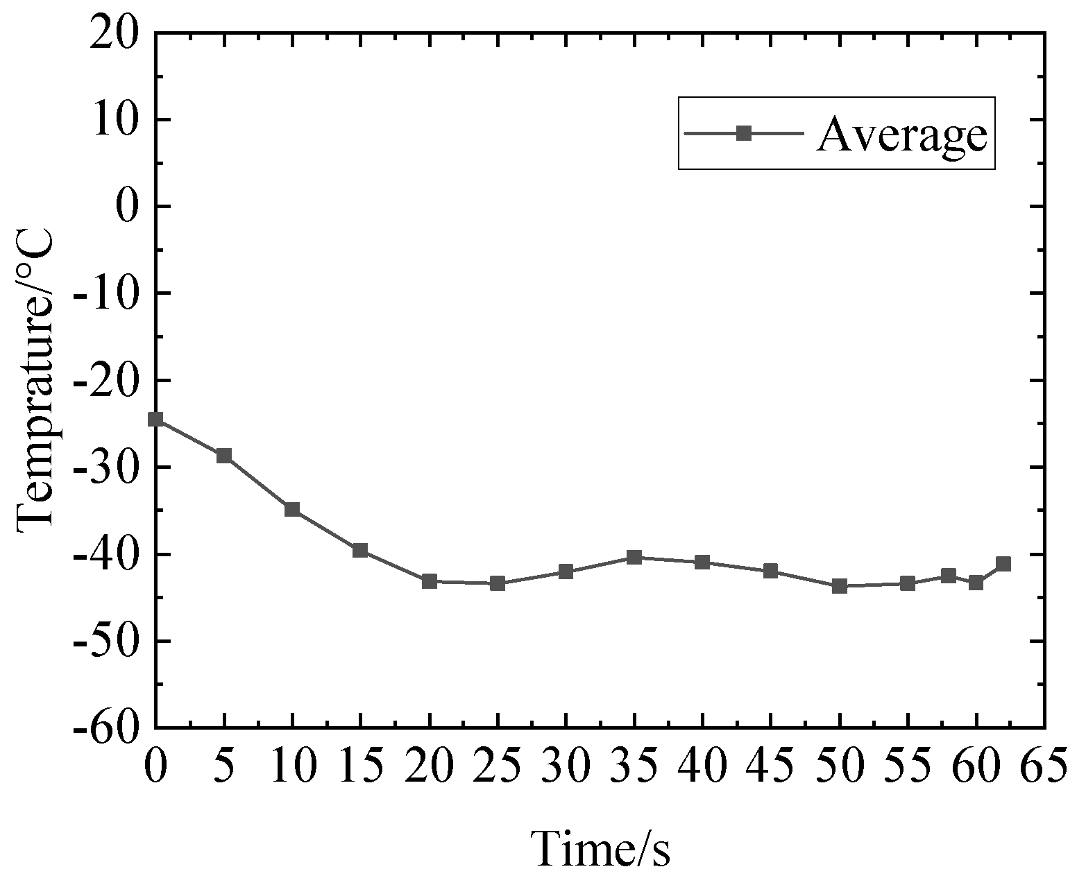
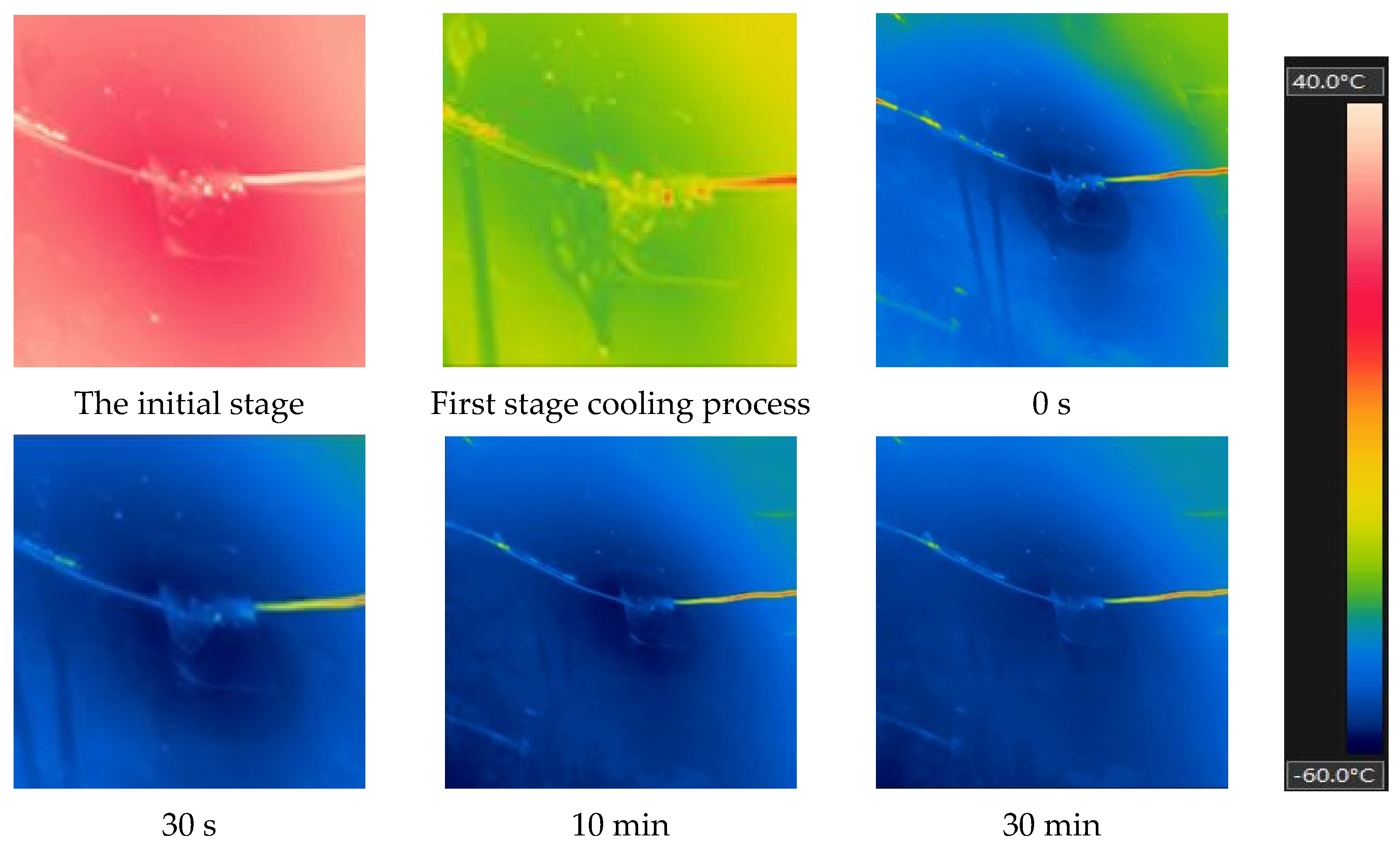
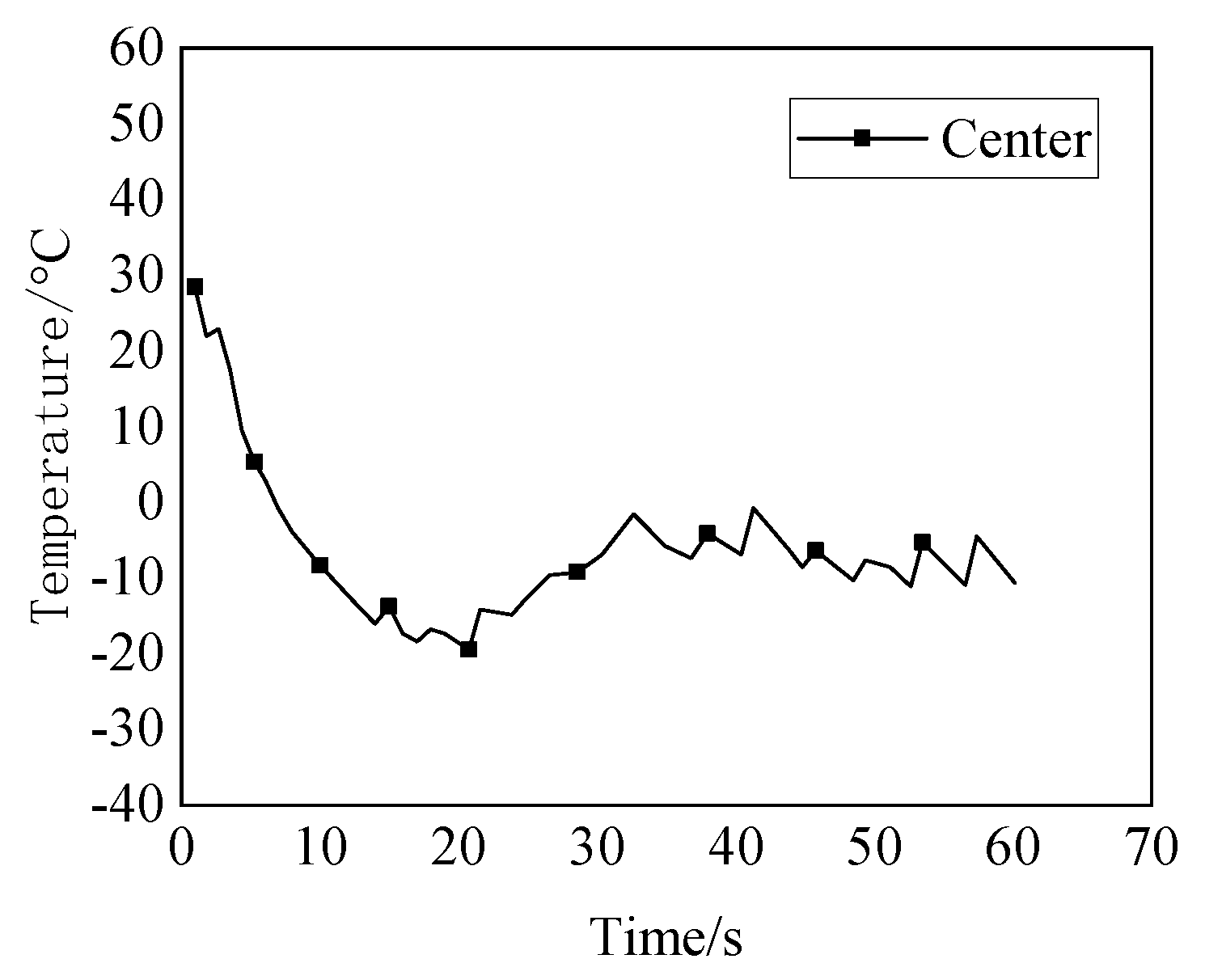
The curve of the regional average temperature change and the infrared image variation with time in the response phase is shown in Figure 10 and Figure 11, respectively. Note that the timing in Figure 11 starts from the quick response phase. Since it is not convenient to determine the start time of the rapid response phase in the whole process, the timing rules are redefined.

It can be seen from the data in

Table 6. Variation of average temperature over time in the response stage.

Time (s)	0	5	10	15	20	25	30	35
Temperature (°C)	−24.5	−28.7	−34.9	−39.6	−43.2	−43.4	−42.1	−40.4
Time (s)	40	45	50	55	58	60	62
Temperature (°C)	−41	−42	−43.7	−43.4	−42.5	−43.3	−41.2

that the cooling has been achieved after 20 s, and the average temperature fluctuations were within −42 ± 1.5 °C after stabilization. After stabilization, the opening and closing period of the solenoid valve remained 8 s, and the time of opening and closing is about 1 s. Exit temperature remained from −60 °C to −70 °C after stabilization. The temperature dropped to −60 °C when the solenoid valve closed and to −70 °C when the solenoid valve opened. The required liquid nitrogen flow rate to maintain the heat flux of 400 W/m² was estimated to be 0.18 L/min through the temperature recovery time of the aluminium plate and energy conservation in the stable stage. Only 5.54 L of liquid nitrogen was used for 30 min after stabilization.

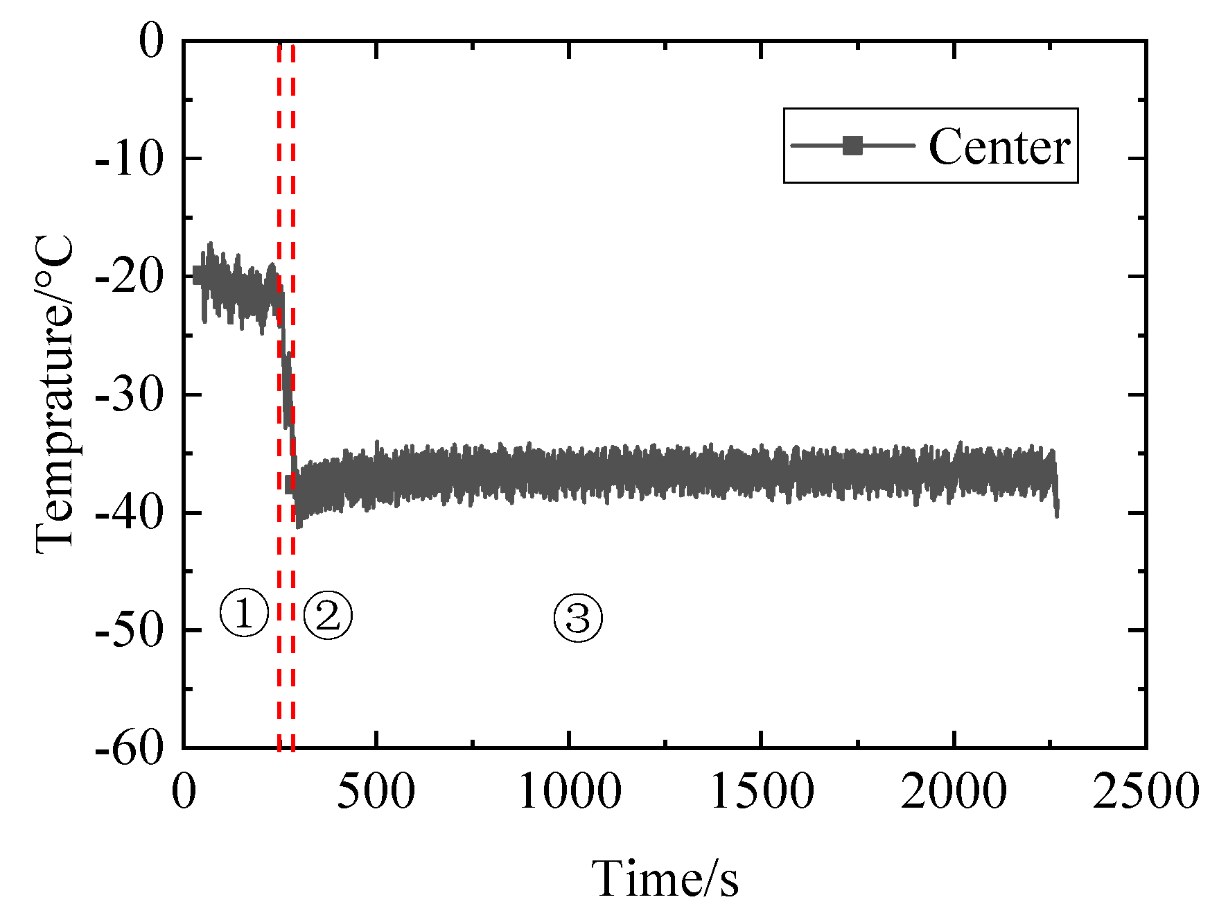
Set the heat flux of working condition 2 as 850 W/m². The heating surface temperature of the thin shell was reduced from −21 °C to −36 °C, and the experimental curve at 0.2 MPa and 850 W/m² is shown in Figure 12. The single point temperature fluctuated within ±3.3 °C after stabilization.

Table 7. Experimental data of three stages under the heat flux of 850 W/m².

	Initial Temperature (°C)		Response Time (s)	Time Required for Stabilization (s)	Stable Temperature (°C)
	Average	Deviation			Average	Deviation
Center	−21.6	±1.2%	<2	33	−36.7	±1.4%

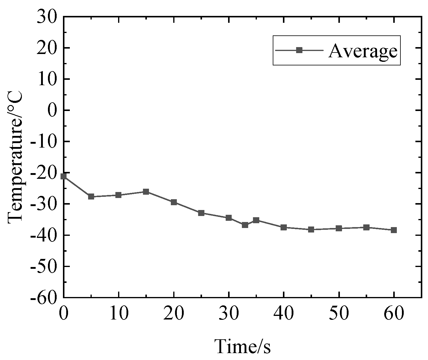
shows the experimental data of the three stages under the heat flux of 850 W/m². The curve of regional average temperature change in the response phase is shown in Figure 13. It can be seen from the data in the table that the aluminium plate has achieved cooling at 33 s, and the average temperature fluctuation after stabilization is within −36.7 ± 1.4%. The response stage is slightly different from the curve under the heat flux of 400 W/m², and there exists a stationary curve. The reason is that the parameters of the self-tuning PID are memorized. In the transition from the first stationary stage to the response stage, there will be a delay in parameter adjustment, making the solenoid valve open and close once. After stabilization, the opening and closing period of the solenoid valve remains 4 s and the opening and closing time is around 2 s.

After stabilization, the outlet temperature is maintained between −60 °C and −70 °C. The temperature dropped to −60 °C when the solenoid valve closed and to −70 °C when the solenoid valve opened. The required liquid nitrogen flow rate to maintain the heat flux of 850 W/m² was estimated to be 0.36 L/min through the temperature recovery time of the aluminum plate and energy conservation in the stable stage. Only 11.07 L of liquid nitrogen was used for 30 min after stabilization. Figure 14 shows the infrared image changing with time.

4.3. Spray Cooling Experiment under High Heat Flux Condition

At a heat flux of 6200 W/m², the temperature decreased from 31.9 °C to −9 °C, and the response time was 30 s. The temperature deviation in the stable stage was +2.2%/−2.3%. The change curve of temperature over time with the decrease of 40 K under 6200 W/m² is shown in Figure 15. The variation of temperature over time in the response stage is shown in Figure 16.

Table 8. Experimental data of three stages under 6200 W/m² heat flux.

Heat Flux (W/m2)	Initial Temperature (°C)		Response Time (s)	Time Required for Stabilization (s)	Stable Temperature (°C)
	Average	Deviation			Average	Deviation
6200	31.9	+2.0%/−1.2%	<2	30	−9	+2.2%/−2.3%

shows the three stage experimental data under 6200 W/m² heat flux.

Under the condition of 6200 W/m², after the stability of temperature on the heating surface of the light thin shell structure, the outlet temperature can be controlled from −60 °C to −70 °C. The temperature dropped to −60 °C when the solenoid valve was closed, and the temperature dropped to −70 °C when the solenoid valve was open. The required liquid nitrogen flow rate to maintain the heat flux of 6200 W/m² was estimated to be 0.37 L/min through the temperature recovery time of the aluminum plate and energy conservation in the stable stage. Only 11.29 L of liquid nitrogen was used for 30 min after stabilization. After stabilization, the opening and closing period of the solenoid valve remains 4.5 s, and the opening and closing time is around 2 s.

Under the heat flux of 10,000 W/m², the temperature decreased from 29.9 °C to −11.48 °C, and the response time was 59 s. The temperature deviation in the stable stage was +3.4%/−1.5%. It can be seen that when the heat flux increases and the solenoid valve is closed, there is no liquid attached to the inner surface. The temperature rise deviation is greater than that under 6200 W/m², and the temperature fluctuation is stronger than that under a small heat flux. The change curve of temperature over time with the decrease of 40 K under 10,000 W/m² heat flux is shown in Figure 17. The change curve of temperature over time in the response stage is shown in Figure 18.

Table 9. Experimental data of three stages under the heat flux of 10,000 W/m².

Heat Flux (W/m2)	Initial Temperature (°C)		Response Time (s)	Time Required for Stabilization (s)	Stable Temperature (°C)
	Average	Deviation			Average	Deviation
10,000	34.3	+1.8%/−1.2%	<2	59	−10.68	+3.4%/−1.5%

shows the experimental data of three stages under 10,000 W/m² heat flux.

Under the heat flux of 10,000 W/m², after the aluminum plate surface temperature stabilized, the exit temperature could be controlled within −110 °C to −120 °C. When the solenoid valve was closed, the temperature dropped to −110 °C, and when the electromagnetic valve was open, the temperature dropped to −120 °C. The required liquid nitrogen flow rate to maintain the heat flux of 10,000 W/m² was estimated to be 0.56 L/min through the temperature recovery time of the aluminium plate and energy conservation in the stable stage. Only 16.83 L of liquid nitrogen was used for 30 min after stabilization. After stabilization, the opening and closing period of the solenoid valve remains 4 s and the opening and closing time is around 2 s.

5. Conclusions

In this paper, taking into account the mechanism of spray cooling, two-phase flow and heating, and the principle of the measurement system, a large area spray cooling experimental platform for the light and thin shell structure was designed and built. The temperature response measurement and analysis experiments were carried out on the heated surface of a light and thin shell structure with a large area under different heat flow and different temperature boundary conditions. The following conclusions are drawn:

(1)

In the spray cooling experiment under low heat flux and low-temperature drop demand, the temperature of the heated surface of the light thin shell structure was reduced from the theoretical value of −25 °C to −40 °C under the heat flux of 400 W/m². The cooling process took more than 20 s to complete. After stabilization, the average temperature fluctuated within the range of −42 ± 1.5 °C. Under the heat flux of 850 W/m², the heating surface temperature of the light thin shell structure was reduced from the theoretical value of −21 °C to −36 °C. The aluminum plate took more than 30 s to achieve temperature cooling, and after stabilization, the average temperature fluctuation was within the range of −36.7 °C ± 1.4%.

(2)

In the spray cooling experiment under high heat flux and a large temperature drop demand, the temperature of the heated surface of the light thin shell structure was reduced from the theoretical value of 31.9 °C to −9 °C under the heat flux of 6200 W/m². The cooling process took more than 30 s to complete. After stabilization, the average temperature fluctuated within the range of −9 °C ± 2.2%. Under the heat flux of 10,000 W/m², the heating surface temperature of the light and thin shell structure was reduced from the theoretical value of 29.9 °C to −11.48 °C, and the temperature was cooled and stabilized in 59 s. After stabilization, the average temperature fluctuated within the range of −10.68 °C ± 3.5%.

(3)

Under different working conditions, the thermal response time of spray phase change cooling is less than 2 s, the surface cooling temperature stability time is less than 60 s, and the cooling state can be maintained for 30 min.