Abstract
This work focuses on a very important and current problem in the gas field: gas losses in natural gas distribution networks and their impact on the environment, as well as on the company operating the network. The paper starts with a bibliographic study and aims to identify the sources leading to losses, estimate loss volumes, reduce these losses by replacing high-risk pipeline sections, as well as trace the economic, environmental, and social impact. The calculation methodologies used in various countries in estimating these consumptions are very diverse. Romania uses a very dense methodology that can prompt very broad variations in the values obtained for technological consumption calculations using Order 18/2014, due to the multitude of parameters that must be estimated. To reduce some of the uncertainties in estimating these parameters, a study was proposed and carried out on the ill-fittings in the natural gas distribution systems. The article presents the experimental stand, the analysis of the experimental data, the methodology for calculating gas losses in the natural gas distribution system through leaking equipment, as well as the results obtained and the conclusions. Moreover, an application was made for a dynamic area check of the gas balance. Based on the correlations between the annual values in M&R stations, AMR, the volume for small consumers, technological consumption, linepack, and the equipment and materials used in the network, useful data were obtained in the diagnosis of problem areas. The end of the paper shows an economic calculation regarding the replacement of problematic pipeline sections in natural gas distribution networks. The difference between the volume of investments and the income from loss reduction is very large, but the aspect of protecting the environment and eliminating technological risks intervenes, thus increasing social security and health.
1. Introduction
The geopolitical issue, including Russia’s decision to cut off gas supplies, has severe and direct implications for European energy security.
Limiting access to imported volumes has a direct and immediate impact on the evolution of both gas and electricity prices, which has implications for the most vulnerable in the population.
This year, reference prices for natural gas traded in Europe are heading towards their longest series of weekly increases, putting more pressure on household consumers and businesses, thus threatening to push EU Member States’ economies into recession.
Quotes have risen continuously over the past year, leading to further market stress. The drought has reduced the production of hydro and nuclear power [1]. As a result, the demand for natural gas is growing at a time when supplies from Russia are falling.
Abnormally hot and dry weather is likely to multiply Europe’s energy crisis in the short term [2], with reduced supply sources escalating the demand for gas and increasing the pressure on energy prices. The main measurable effect of consumption is by far represented by carbon emissions [3], thus implicating an environmental impact as well as an impact on social health.
The price of electricity will also be affected by rising gas prices. Why is such a phenomenon plausible? Because, amidst drought and low quantities of hydro and nuclear power, gas power plants are being switched on to meet the electricity needs. The price is then adjusted on the stock exchange according to the highest one; in this case, the price of gas has powered electricity.
In this complex context of influencing factors, the issue of gas leaks in distribution systems is of particular importance, as it negatively affects the balance sheet of distribution companies, pollutes the environment, and also represents a major risk due to the formation of explosive mixtures in the presence of air, especially if we use hydrogen mixed with natural gas [4]. The transition to a green economy will ensure the development of a low carbon economy in the context of efficiency considering the facilities generated by digitalisation [5].
As evidenced in Figure 1, based on 140 papers from the Web of Science, there are studies in the literature on the simulation of natural gas leaks in the transmission of natural gas and distribution networks, which resulted in both the keywords that best characterise the research in this article and the links between them: natural gas leakage, pipelines network, experimental model, environmental emissions, and economic.
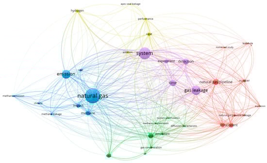
Figure 1.
Common words in scientific publications (source: authors, based on articles analysed).
No study/survey in the numerous articles in the literature review has brought together all of these complex issues to use in running a techno-economic profitability study on the opportunity of investments in replacing old or outdated pipelines, nor has it provided a presentation of the environmental impacts these investments could have.
The following is a bibliographical survey of just a few works which have dealt with the issue separately, but have shared objectives with this paper.
Lustenberger P., Schumacher F., Spada M., Burgherr P., and Stojadinovic B., in the paper Assessing the Performance of the European Natural Gas Network for Selected Supply Disruption Scenarios Using Open-Source Information [6], conducted a study based on a volume of large-scale data dedicated to the European natural gas networks from publicly available information sources. The spatial coverage, completeness, and resolution allowed them to analyse the behaviour of these geospatial infrastructure networks (including consumption) and their components, under likely disruptive events, such as earthquakes and/or technical failures. The disturbances impact was highlighted using the developed system state simulation engine. The results show that storage facilities cannot compensate for the disruption of a pipeline in all cases. In order to analyse pipelines with a high impact on the system performance, a detailed scenario analysis was performed and presented using a Monte Carlo simulation that led to the conclusion that the pipelines were at a dead-end with a single supply source and no nearby storage facility, meaning they were highly exposed to natural gas supply losses.
Dezfouli, A.M., Saffarian, M.R., Behbahani-Nejad, M., and Changizian, M., carried out experimental and numerical research to develop a method for measuring the natural gas loss rate both from domestic gas pipelines branching off from natural gas distribution pipelines, and from their connections, by developing a numerical model of a gas branch based on its real conditions [7]. Through numerical simulations, the researchers have established the general geometry of the model and its various components in order to accurately predict the gas loss flow rate from the output gas concentration value and the numerical solution results were validated, as in the present paper, by using a stand. The volumetric flow rates calculated using the proposed method are extremely close to the real values. In addition, the numerical solution produced results within an acceptable margin of error compared to the experimental results.
Another relevant experimental study on the key issue of how to detect and quantify a pipeline leakage was conducted by Yunpeng Y., Jianchun F., Shengnan W., Di L., and Fanfan M [8]. A pipeline leakage event detection and quantification method based on multiple acoustic feature fusion (MAWF) was proposed. The test results showed that the proposed method could efficiently and quickly identify the leakage condition of pipelines, and the leakage event recognition accuracy measured up to 98.79%. The results of this study helped to improve the early warning time of pipeline leaks.
Accounting for the new trend to use energy mixes with hydrogen, Mejia, N.A.H., and Brouwer, J. conducted a study on the possible means of storing and delivering renewable hydrogen by injecting it into the existing natural gas system and thus decarbonising gas end uses [9]. The natural gas distribution system has a real potential to serve as a storage, transport, and distribution system for hydrogen produced from renewable sources. Despite the potential of hydrogen to reduce the carbon intensity in the natural gas distribution system, the unique characteristics of hydrogen (a low molecular weight, high diffusivity, lower volumetric heat value, and a tendency to embrittle pipeline materials) have led to justified concerns regarding the safety of introducing hydrogen mixtures into the natural gas distribution system.
Hou, Q.M., Jiao, W.L., Zou, and P.H. have analysed the leakage and diffusion characteristics of natural gas [10]. According to the results, when natural gas leaks from pipelines, it dissipates into the atmosphere as positively buoyant jets. As a result, a danger zone can occur at an altitude of 150 m above the ground. In addition, natural gas has a low concentration close to the ground, which means that natural gas is less harmful to the human body. Moreover, when transporting leaked natural gas, wind must be taken into account.
Even if they are not intended for gas distribution systems, a wide variety of methods are presented in the literature in order to analyse pipeline systems in terms of their failures, lifetime, and susceptibility to failures based on statistical analyses and operational research using predictions of fluid transport. As the present study will emphasise, it is very useful to validate these methods using real stands and/or equipment [11,12].
Of course, there is a great deal of literature in this strategically important area, which is why we must stress the importance of the present paper, in which the authors propose a combined study of the issue of gas leaks in a distribution network of a major commercial agent.
The issue of gas leaks is treated in a complex manner, taking into account the number of factors influencing the natural gas distribution activities, starting from the identification of the sources leading to leaks [13], the identification of leak volumes, the methods of reducing these leaks by replacing long service life pipeline sections, as well as the economic and environmental impact of these preventive activities.
As a consequence of the above, and to more easily highlight the methods of carrying out the research, Figure 2 illustrates the graphical abstract of the content of this article.
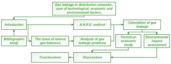
Figure 2.
Graphical abstract (source: authors based on research data).
As one can see in the graphical summary of the article, the topics covered in the following chapters present the contributions to the field of gas leaks:
- The research topic dealt with in this study is a highly topical one in the field of natural gas: a gas leakage in natural gas distribution networks and its impact on the environment, as well as on the economic component of the distribution company operating the network.
- It has been found, after a highly careful analysis of the bibliographic study, that not many articles validate experimentally the methods used, but they only deal with technical issues without considering other aspects of risks caused by fluid leaks in distribution networks.
- As it will be shown in the article, the main contributions of the article are relevant and consist of: the use of a complex experimental stand to identify the leakage volumes through the equipment from the distribution systems, the simulation of the total leakages, based on the results for the whole distribution network, split by balance areas, and their impact on the environment.
Gas losses can be physical losses representing a gas leakage from distribution systems into the environment, or they can be indirect or technological losses due to imperfections in metering systems. Indirect gas losses are influenced by variations in the atmospheric parameters, pressure and temperature, in the vicinity of the measurement point [14]. According to the new Romanian legislation represented by the Network Code, direct and indirect gas losses affect the gas allocations that the company makes to the National Transmission Company. A large inaccuracy in defining these gas allocations leads to penalties for the distribution company.
In the European Union, gas released/emanated from distribution systems accounts for about 80% of the methane released into the atmosphere. These emissions have a high impact on the environment and quality of life.
Methane emissions as a result of the activities of the gas industry are caused by the routine operation of pipeline networks, routine maintenance, system failure, and external factors. Methane emissions from gas networks can be divided into four broad categories: fugitive/occasional emissions, emissions from pneumatic devices, vented emissions, and incomplete combustion emissions.
However, gas losses are not measured directly but estimated according to various existing methodologies. Such estimates are known to be relatively inaccurate and require further efforts to improve their accuracy, both in terms of global emissions as well as their distribution in different countries. In addition to their importance in assessing and controlling global climate change, the knowledge of methane emissions from natural gas distribution networks is essential for distribution companies seeking solutions to reduce a gas leakage.
The emissions from the gas distribution are based on the activity factors (e.g., the pipeline length and number of customers) and emission factors for the various types of pipeline materials [15,16].
The emissions from service lines should be calculated by choosing one of the following two alternatives:
- By selecting an emission factor and multiplying by the number of customers (the activity factor).
- By selecting a value between 20% and 90% of the emissions from distribution lines.
The actual operating energy regimes of the natural gas distribution networks were determined using historical data, the energy parameters, and information from specialists.
The components of the volumetric, mass, and energy balances, gas and energy losses, and the real and specific energy consumption were calculated, using specific equations involving the values of the measured parameters [17].
The analysis of the real energy balance will lead to locating unknown losses, determining their causes, and identifying the measures to be applied in order to improve and optimise the technical-economic indicators [18]. All balance sheet data should be compared with previous balance sheets, project data, and other data from similar economic operators or the literature.
2. Problem Presentation
Gas losses through pipeline defects into the external environment fall into two broad categories: losses through overhead pipeline defects and losses through underground pipeline defects. In the case of a leakage through overhead pipeline defects, the gas loss can be modelled with analytical relationships. For these cases, the flow through the defect is limited to the critical flow rate at the time when the flow becomes critical, otherwise the flow rate depends on the defect cross-section and the pressure difference. For buried pipelines, the pipeline defect is basically plugged by the soil. The gases escaping through the defect depend on the properties of the soil around the pipe, and the phenomenon physically represents the diffusion of gases through the porous medium, depending on its permeability and porosity [19].
From the numerical analysis conducted for buried pipelines, it appears that regardless of the position of the defect, the gas pressure variation in the vicinity of the defect is very quick, over a small space of 25–30 mm. For this reason, the pressure gradient in this area was considered determinant for the gas flow through the defect.
The main problems causing errors in metering systems are related to the lack of gas volume correction when using mechanical volumetric meters for households or small businesses [20]. These errors occurring in metering systems depend on the temperature and atmospheric pressure.
Another problem related to gas metering systems is the long-time interval between two readings, which is one month, during which the atmospheric parameters’ pressure and temperature vary a lot, leading to a correction of the monthly volumes consumed using the monthly average values for the temperature and normal pressure corrected by the altitude [14].
The analysis of the contribution of the atmospheric temperature and pressure variation in the level of error shows that temperature is the determining factor. However, the level of errors calculated from the in situ measured data shows that it is higher. This difference is due to consumption dynamics. Experimental research has shown that the gas temperature at the measuring point (gas meter) is identical to the atmospheric air temperature. Experimental research on the atmospheric pressure has shown that its daily average values are below the normal pressure corrected for the altitude.
In Romania, the calculation for the technological consumption in natural gas distribution systems is based on a calculation methodology provided by the ANRE (National Authority for Energy Regulations) [21,22,23].
This methodology for determining the technological consumption in natural gas distribution systems takes into account the volumes of natural gas necessary to fill a new section or to increase the working pressure, lost in the atmosphere through overhead or underground defects, technical incidents through a total or partial pipeline rupture, dissipated due to the permeability of polyethylene pipelines and due to the conversion to converterless equipment/metering systems.
Due to the many problems of closing the volumetric balance for certain areas, it was concluded that the calculation methodology used to estimate these consumptions may give erroneous results. Due to the multitude of parameters to be estimated (the pressure, temperature, gas volume, gas composition, flow coefficients, defects area, soil permeability and subsidence, pipeline length until first valve, and the average atmospheric temperature and pressure) and their variation in time, there can be great variations in the values obtained from the technological consumption calculations using Order 18/2014. To reduce uncertainties, a study on the ill-fittings in natural gas distribution systems was proposed and carried out.
The paper presents the experimental stand, the analysis of the experimental data, the methodology for calculating gas losses in the natural gas distribution system for ill-fitted equipment, the results obtained, and the conclusions. In order to make the results as relevant as possible, the natural gas was treated as a mixture of real gases with the composition defined in the chromatographic bulletin. Based on this, the properties of the gas mixture were calculated and used for the evaluation of different types of losses.
The gas flow rates were calculated on the basis of formulas, whereby an exponential relationship conditioned by the flow rate was admitted for the hydraulic head loss coefficient.
Thus, the details of the construction, fitting the experimental stand, the experiments carried out, as well as a method for calculating the volumes of gas lost due to defects of this type are presented. Beginning with the calculation of the properties of natural gases depending on their chromatographic composition [24], the values obtained for the analysed technological losses and verified by the prepared software are presented. The gas flow rates lost through these types of defects were determined depending on the defect area. The present paper presents a summary of the losses through defects in ill-fitted equipment and the total losses in a natural gas distribution network.
Using the results of the study, the total technological consumption was recalculated, the impact inside the network was tracked, and measures to reduce atmospheric emissions were proposed.
In order to estimate the environmental impact, the CO2 equivalent quantity was calculated based on the amount of natural gas lost from the system.
It was considered necessary to analyse, through an economic calculation, the recovery, from the costs of purchasing gas volumes, of the investment for the replacement of faulty pipelines if these loses are not corrected.
3. Gas Losses from Distribution Systems
Although gas losses in the distribution network are caused by the above-mentioned factors, information on the total amount of losses is difficult to establish, because the exact volume of many losses cannot be specified, due to uncertainties and coincidences. Simply adding different elements could lead to an over- or underestimation of the actual value. To overcome this “problem”, European operators of gas distribution systems use a more general method of loss estimation. Depending on the choice of each country, one or more of the factors discussed above can be used as the evaluation methods of estimated methane emissions.
Methane emissions are insignificant compared to the volume of gas distributed. The volume of emanations cannot be measured directly, but it can be estimated as we describe below. The estimate calculation is very complex. Specialised studies (IPCC, US EPA-GRI, IGU, CORINAIR, FRAUNHOFER, and BATTELLE) describe different methodologies for estimating methane emissions [15,16,20,25,26,27,28]. Although they propose different approaches, all the methods are based on the following equation:
Emissions = Σ (Activity factor × Emission factor)
MARCOGAZ WG proposed a common methodology for calculating methane emissions. A working group from MARCOGAZ has published a common methodology outlining the best practices to be addressed in the European gas industry [15]. This method was evaluated by a comparison with the existing data.
The application of such an algorithm is very fast and does not require the analysis of huge volumes of data and personnel dedicated to technological loss calculations, and the results are similar to those obtained through the current methodology.
3.1. Gas Losses Due to Faults in the Distribution System—ANRE Methodology
The calculation and reporting of the technological consumption from natural gas distribution systems is carried out based on the ORDER for the approval of the methodology for calculating the technological consumption from natural gas distribution systems, published in the Official Gazette of Romania, Part I, No. 226/31.III.2014 and subsequent additions [21,22,23]. The results of the calculations are provided in Excel spreadsheets according to the format required for reporting to the ANRE [23].
According to the methodology for determining the technological consumption in natural gas distribution systems, the volumes that must be reported to the ANRE are grouped into seven items, as follows:
- Art. 6—The volume of natural gas required to fill a new DS section to ensure the working pressure of new or rehabilitated pipeline sections;
- Art. 7—The volume of natural gas injected into the existing DS, as a result of the DSOs decision to increase the working pressure;
- Art. 8—The volume of natural gas dissipated in the atmosphere due to defects in the DS equipment, mounted above ground;
- Art. 9—The volume of natural gas dissipated in the ground due to defects in the DS equipment installed underground;
- Art. 10—The volume of natural gas dissipated as a result of technical incidents in the DS manifested in the total or partial rupture of the pipeline;
- Art. 11—The annual volume of natural gas dissipated as a result of the permeability of polyethylene pipes;
- Art. 12—The volume of natural gas required to be purchased as a result of the difference between the volume of natural gas expressed in standard conditions of temperature and pressure and that delivered by measuring equipment/systems without a converter.
Based on the real, local properties of the gases delivered through M&Rs such as the composition, molecular mass, compressibility factor [29], specific heat, adiabatic exponent, viscosity, etc., gas losses are determined by a calculation, defect by defect. Gas losses for overhead or buried pipelines are specifically treated. One can calculate, using the methodology approved by the ANRE [23], the losses due to the technological processes of filling/emptying the pipes and the rupture of the pipes through meters without a corrector. Furthermore, non-localised losses due to the pipe’s permeability, and losses due to ill-fitting or maintenance work must be accounted for as well.
Next, the results of technological loss calculations according to the ANREs methodology [21,22] will be presented.
Thus, in Figure 3, one can see the daily variations in the losses for each category. It can be seen that the aerial defects (article 8 of the ANRE methodology) and volume correction due to measurements with equipment without a converter (article 12) constitute the biggest share.
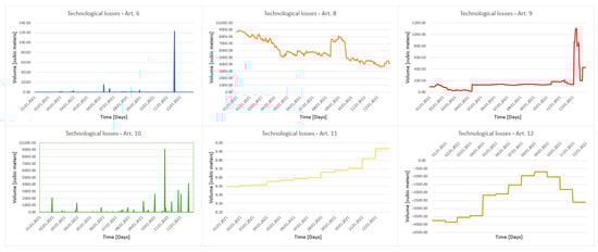
Figure 3.
Structure of losses by types (source: authors based on the analysed data).
In addition, the peaks standing out must be identified, analysed, and verified.
Figure 4 shows all the technological losses calculated according to the ANREs methodology.
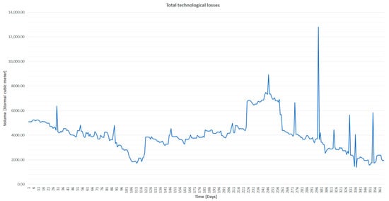
Figure 4.
Technological losses in accordance to ANRE—year 2021—balance area (source: authors based on the analysed data).
The annual volumes lost in the atmosphere, divided by the types of defects (articles) in 2021 can be found in the Table 1.

Table 1.
The annual volumes lost in the atmosphere (source: authors).
Moreover, the losses were assigned to the balance areas for a better analysis of the problems in the system and in order to achieve the volumetric and energy balance.
Following the analysis of the volumetric balance in these areas, major non-closures were found, a sign that the current calculation methodology or the parameters used in the calculation are not correct. The network equipment data were analysed and correlations were made between the annual values of M&R, AMR, the Profiled Volumes and Losses associated with M&R, and the network characteristics (No. of valves, regulating points, lengths, and their subcategories).
Based on the analyses conducted, it seems that the volumes calculated for losses through surface defects are overestimated, while the volumes infiltrated through the soil from underground defects are underestimated. To clarify these aspects, studies were considered necessary, and were proposed, regarding the assessment of these two categories of losses. The results of the study on the defects due to ill-fitting are presented in the following sections, with the other types of faults being reserved for future analyses.
3.2. Gas Losses Due to Ill-Fitted Equipment Defects in the Distribution System
Part of the technological consumption is represented by gas losses due to ill-fitted equipment defects in natural gas distribution systems. The analysis of these losses was performed on the basis of a relevant data set, provided by the network distribution operator, following the experiments conducted.
The gas losses were analysed as follows:
- The creation of an experimental stand that allows for the measurement of certain hydrodynamic flow parameters.
- A numerical model was created, that was attached to the experimental device to allow for the calculation of the volumes of gases leaked due to the defects of ill-fitted equipment in the distribution system.
- The calibration of the flow coefficients of the defect by comparing the experimental data with theoretical ones.
- The realisation of a method for calculating gas leaks due to ill-fitted equipment defects in the distribution system for other pressure regimes practiced by the network distribution operator.
3.2.1. Description of the Experimental Device
The experimental device was created to determine the gas leaks due to the defects of ill-fitted equipment in the distribution system, to determine the flow regime and to calibrate the flow coefficients. It consists of a pipe with a diameter of D = 6” and a length of 6 m. The gas supply was made through a connection with a diameter of Dn = 50 mm and a length of 2.5 m. The maximum loading pressure of the experimental device is 4.5 bar. The pressure measurement in the system will be carried out with the absolute pressure transducer of a rotary piston counter equipped with a converter with the recording time set to 1 min. The experimental stand is presented in Figure 5.
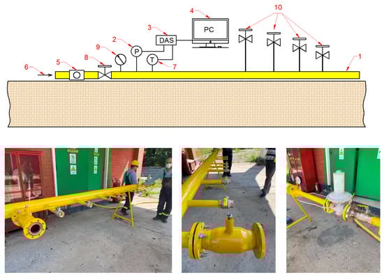
Figure 5.
Experimental stand structure for losses due to ill-fitting (1—pipe coupon with a minimum diameter of 150 mm and a length of 6 m, 2—pressure transducer, 3—data acquisition system, 4—pressure-time recording system, usually with PC, 5—flow meter with rotating pistons, 6—gas source, 7—temperature transducer, 8—faucet, 9—pressure gauge, 10—various types of equipment) (source: authors based on the real analysed equipment).
In the pipeline, defects due to the ill-fitting of various sizes were used separately. For each type of defect, the pipe was loaded through the gas supply system at 4 bar, then the pressure variation was measured using a pressure transducer during the emptying of the pipe through the ill-fitting. In addition, a set of tests were carried out in the event of a pressure regulator with the pressure set to 1.2 bar.
3.2.2. Methodology for Determining the Volume of Gas Lost through Ill-Fittings
An experimental stand is used to determine the volumes of gas lost through ill-fittings. The stand consists of a chamber of a known volume into which the gas of a known composition is introduced at a measured pressure. A nozzle with the analysed defect is connected to the experimental volume. Due to the gas leakage through the defect, the pressure in the stand volume decreases over time. The length of the experiments is different, depending on the size of the ill-fitting, the degree of tightness in the ill-fitted area. For the same type of faulty fitting, the experiment was repeated for several different diameters.
A hydro-thermodynamic model applied to the stand is used to determine the gas flow outpouring through the defect.
The gas equation of the state is:
where:
- p—is the natural gas pressure in pipeline [bar];
- V—the volume of gas [m3];
- m—the mass [kg];
- Z—the compressibility factor;
- R—the universal (ideal) gas constant [J/(mol∙K)];
- T—the temperature [K].
We consider to be the gas mass flow rate through the defect.
During the experiment, the absolute pressure in the experimental device and the temperature were measured with a sampling step of 1 min.
We consider the gas equation of the state written for two successive time moments τ and τ + Δτ.
From the two relations, we can deduce the mass flow rate lost through the defect depending on the pressure and temperature variation according to the relation:
Each experiment ends with pressure and temperature values collected during its duration and stored in a file. For the ½ in the defect, we present an example from the data sample in Table 2.
Table 2.
Measured gas parameters (source: authors).
3.2.3. The Method of Calculating the Gas Volumes Lost through These Types of Defects
Since the phenomenon of a gas leakage through defects is particularly complex, a thermo-hydrodynamic model of pipe emptying was created that generates a theoretical curve of pressure variation in the pipe for each type of defect. The coefficients for each type of defect were calibrated by comparing the experimental and the theoretical curves, leading to a formula for calculating losses due to defects.
The pressure in the pipe is considered to be uniform, but due to the small volume of the experimental pipe (8 m long) and the high dynamics of the phenomenon, it is possible that in the vicinity of the defect the pressure in the pipe is a little different from the average pressure measured at the measuring point. Another problem that partially affects the results is the sampling rate of the measured values (1 min). This was achieved by programming the purchase time from the meter, a very useful thing.
The experimental determinations proceed as follows:
- Fill the pipe with gas to the desired pressure;
- Use an ill-fitted defect with a certain equivalent diameter (surface);
- Close the pipeline supply;
- Measure the pressure variation in the pipeline when it is being emptied.
The pressure curve which resulted from the gas leak is compared to the pressure curve which resulted from a model of a faulty gas flow. By comparing the two curves, the corresponding flow coefficients are determined.
The flow which resulted from an ill-fitting can be calculated with Formula (4) that relates the parameters of the gas in the pipe (p, T) to the area of the defect and to the properties of the gas.
Formulas (6)–(8) relate the mass flow rate to the volume flow rate under standard conditions of pressure and temperature.
3.2.4. Experimental Data Processing
To process the experimental data, a software was created that allows for the quick collection of the results. The properties of the components used are the usual ones in the specialised literature. The software automatically loads the gas composition and calculates the main parameters, the apparent molecular mass of the mixture, the isobaric specific heat, and the adiabatic exponent, which are the critical parameters. The data from the chromatographic analysis bulletin in the processing software were used for the composition of the gases.
From an experimental point of view, the gas losses of the ill-fitted equipment in the distribution system located at the end of the test pipeline were analysed. After the pipeline was loaded with gas, three experiments were carried out by expanding the faulty fitting. The two elements necessary for this step were the pipe’s diameter and the number of unscrewing rotations, meaning 2, 5, 3, and 4 turns out of a maximum of 5 possible turns. The results of the functions representing the pressure drop are similar to those presented below.
In order to evaluate the gas losses, an attempt will be made to associate these gas losses with the other phenomena already studied (leaks through defects), but it was found that these type of leaks, through ill-fittings, have a particular aspect. In this case, the gas flow through the ill-fitting will be determined directly from the experimental data and a function will be assigned to it.
Ill-Fitted Equipment on a 1″ Pipe
The data files downloaded from the PTZ converter meter resulted in segments of data depending on how the measurements were performed. These data segments, Figure 6a, are processed in order to remove the deviations produced by the measurement and processing method to detect trends.
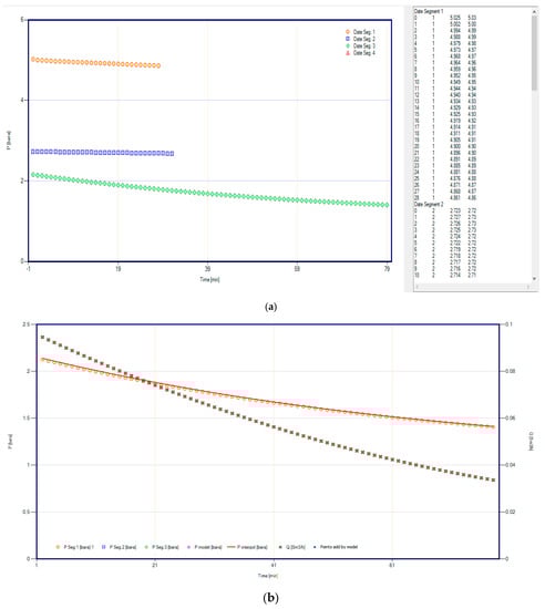
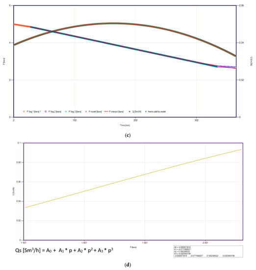
Figure 6.
Data processing stages: (a) experimental data for 1 in and 3 turns ill-fitting; (b,c) curves modelled for pressure and calculated flow; (d) flow—pressure variation for 1 in and 3 turns—adjusted pressure (source: authors based on the analysed data).
For the medium pressure area, usually two segments of measurements were made, thus resulting in two segments of data. As a rule, these two data segments were processed unitarily, Figure 6, resulting in the pressure variation and the flow variation through the defect.
For low pressures, usually below 1.2 bar, the measurements were carried out continuously, resulting in a data segment specific to this area.
The experiments were carried out over different periods of time. The curves presented so far have been processed according to the time axis.
In order to make the results relevant and usable later, time was removed from the series produced by the measurements, resulting in a pressure-flow data series. In order to be able to determine the relationship between the pressure and the flow lost through the defect, the curves were modelled with polynomials, thus resulting in a relationship between the pressure in the installation and the gas flow lost through the defect, Figure 6c.
The model used is based on the thermo-hydrodynamic formulas which resulted from the gas flow theory. The calibration of these models with the experimental data is performed by determining some values of the flow coefficients, so that the error between the two curves is minimal.
Use the obtained results as follows. Depending on the size of the ill-fitting (equivalent diameter), the pressure regime and the temperature in the pipelines, the theoretical calculation formulas calibrated with the experimentally determined flow coefficients are used to calculate the volumes of gas lost through the defect.
Using the flow rates calculated from the experimental data and modelled by the function (from Figure 6c), the experimentally determined pressure variation curve will be regenerated for a verification and comparison (Figure 6b). It will be found that the model used describes the phenomenon very well.
Benchmarking
For other ill-fitted equipment, the procedure will be similar. The following steps will show some comparative graphs for various faulty fittings on the same pipe or on different pipes, as presented in Figure 7.
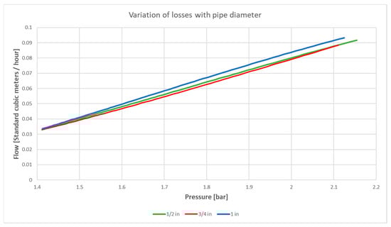
Figure 7.
Comparative analysis of flow for different diameters (source: authors based on the analysed data).
After analysing all the flow rate variation curves with the pressure, it was found that due to the factors of various causes, some curves are not relevant throughout the field, causing some overlaps. For this reason, it was considered necessary for some of these curves to be corrected, to fit with the others. Figure 8 illustrates such a case.
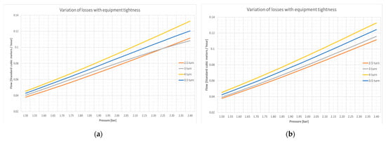
Figure 8.
Correction of a flow rate variation curve with pressure and leakage faulty fitting (a) real data curve; (b) revised curve. (source: authors based on the analysed data).
Simplified Calculation of Gas Volumes Lost Trough
Since it is difficult to compare the real gas leaks with a faulty fitting of several sizes, considering the experimental data and the results obtained by numerical modelling, a more general case was considered in order to capitalise on these results.
Considering the experimental results presented previously, the flow coefficients were mediated because the operating pressures of the network distribution operator vary. A function was thus achieved that generates the flow coefficient of the defect that depends only on the pressure in the pipe.
Since this case might also be difficult to work on in on-site conditions, a model for faulty fitting was defined, in which the leaking flow rate is the average of the analysed cases for each pressure regime. Given that losses through faulty fittings can occur anywhere in the network, in order to be able to calculate the flows lost through them and at pressures other than those analysed experimentally, the average flow function was extrapolated. Thus, using Figure 9 and Figure 10, it is possible to calculate the flow rates lost due to ill-fitting at various pressures.
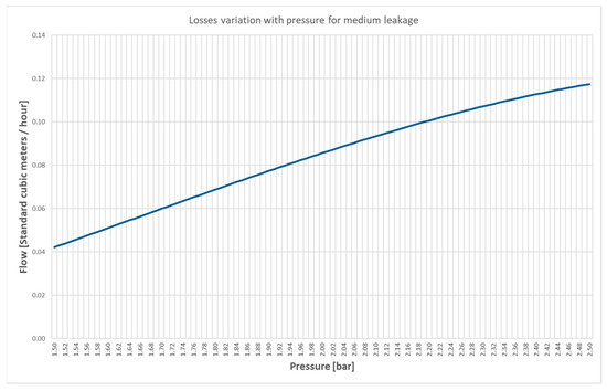
Figure 9.
Variation in lost flow as a function of reduced pressure for medium faulty fitting (source: authors based on the analysed data).
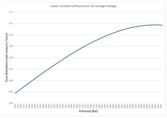
Figure 10.
Variation in lost gas flow rate as a function of average pressure for average faulty fitting (source: authors based on the analysed data).
Considering that in the distribution system there are also pipes of diameters larger than 2 in, the values obtained through calculations for the 3, 4, 6, and 8 in diameters were extrapolated.
4. Technical and Economic Study
Analysing in detail the volumetric and energy balances for each area, many anomalies can be observed, some of which have logical explanations.
The following Table 3 summarises the total gas losses and the volumetric balance resulting from calculations corrected for ill-fittings. The share of energy consumption shows acceptable values of non-closures.
Table 3.
Total losses and volumetric balance (source: authors based on the analysed data).
Losses of gas in the system mean costs for the distributor to replace the lost gas and to assess the environmental problems caused. Fixing or replacing pipelines in areas with many faults leads, over time, to a reduction in these costs.
In order to estimate the environmental impact, a CO2 equivalent was calculated based on the amount of natural gas lost from the system, using an emission factor of 1 m3 of natural gas = 1.9 kg CO2. The volume of the technological losses was calculated in two ways: as a volume of the total losses and as a volume obtained by adding items 6–11 of the current technological loss calculation standard. Article 12 is not taken into account because it represents a correction of the meter readings.
The calculations resulted in the following annual air emission values expressed in tonnes CO2 equivalent (Table 4).
Table 4.
CO2 equivalent per year (source: authors based on the analysed data).
In the present study, an economic estimate is presented, based on two scenarios, for the replacement of outdated pipeline sections in natural gas networks. From the statistical studies carried out on the economic agent’s readings, it was revealed that the highest volume losses during the transport of natural gas through pipeline systems are recorded on the sections with a long service life in this technological process.
These actions are welcome at this stage, due to two important influential factors, namely natural gas prices that are on an upward trend, and the transition to natural gas-hydrogen energy mixes at a global and European level. Eliminating these losses has a beneficial effect in reducing the influence or even eradicating these two factors.
The complexity of the technological processes involved in replacing the elements in pipeline systems, especially sections of tubular material, radically impacts the cost of this work.
According to the data provided by the economic agent, replacing one linear metre, depending on the areas where the pipes are laid out (residential and non-residential, uncovered or covered with asphalt mix or concrete), costs between EUR 100 and 1000.
For the first scenario of this economic study, taking into account the average prices of the main types of material (Steel or HDPE), the lengths of the sections, and the diameters of the tubular pipe material replaced (between 5˝ and 10˝), the reference cost is 300 EUR/lm.
The distribution pipe network, from the commercial agent, is approximately 1815 km long, with a very varied dimensional configuration, pipes of varying lengths, materials and diameters. For this distribution network, the total volume of losses in 2021 was calculated above, at approximately 1,712,504 m3, for which, at an HCV of 10.5 and an average natural gas value of 500 EUR/MWh, the value of these losses amounts to EUR 8,990,646.
As per the presentation above, see Table 5, there is a plan for the next few years to replace several kilometres of pipelines with a long service life.
Table 5.
Lengths in kilometres planned to be replaced (source: authors based on the analysed data).
The economic calculation is based on the simple reasoning that if annual investments are planned in order to replace those sections of the distribution pipes that have a long service life and are even outdated, causing losses, with sections made of new tubular material, the overall loss volume will be reduced. Using this reasoning and the data in the previous paragraphs, an annual summary can be made in terms of: the lengths replaced, amounts invested, and reduction of losses.
Based on the centralised data—scenario 1—the two graphs in Figure 11a,b have been produced, representing the annual variation in the pipeline sections lengths to be replaced, the investment costs incurred by these upgrades, and the reduction in losses as a result of these investments [30].
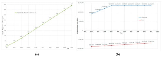
Figure 11.
Lengths replaced, amounts invested and reduction in losses—scenario 1: (a) planning lengths to be replaced, km; (b) investment costs and loss mitigation, EUR (source: authors based on the analysed data).
As can be seen from the representative graphs in Figure 12, the technological process of replacing sections of old distribution pipelines with a long service life or even an outdated service life, which produce considerable losses, implicitly leads to a reduction in the technological losses of the fluid conveyed which, in this case, is natural gas.
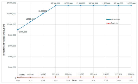
Figure 12.
Volume of investment costs and revenues, EUR—scenario 1 (source: authors based on the analysed data).
Moreover, as can be seen in Figure 12, the investment volume is very high and the returns from reducing losses are quite low, but from the point of view of environmental protection and eliminating technological risk situations, these investments are of a strategic importance.
For scenario 2, the data from the previous scenario are used, with the exception that the annual lengths for the pipeline sections to be replaced are proposed to measure 70 km/year. Another assumption is that replacing most critical sections in distribution pipeline systems reduces the annual losses by a weighted average of 3176 m3/year, different from the previous scenario, where the weighted value of the losses is 943 m3/year.
The data used in scenario 2 take into account the same length of the pipeline network, with a rather diverse dimensional configuration, varying lengths of the pipes, different materials, and diameters.
The data for scenario 2 will be presented in order to have a clearer picture of the benefits of replacing longer lengths of critical, obsolete, or outdated pipeline sections.
It is evident in Figure 13 that increasing the length of critical pipeline sections results in an 18% increase in revenue compared to the previous scenario, which is reflected in the company’s budget, amounting to approximately EUR 11,671,800, compared to EUR 2,081,520.
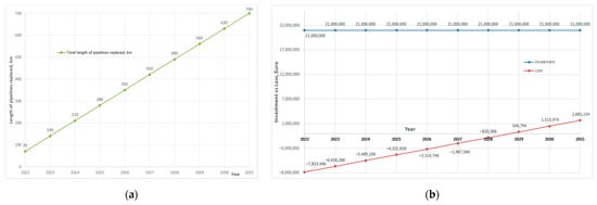
Figure 13.
Lengths replaced, amounts invested and reduction of losses—scenario 2: (a) planning lengths to be replaced, km; (b) investment costs and loss mitigation, EUR (source: authors based on the analysed data).
Scenario 2, as shown in Figure 14, maintains the same conclusion Scenario 1, i.e., that the difference between the volume of the investment and the revenue from the loss mitigation is very large. The main advantages speak about environmental protection and the elimination of technological risks, for which we stress that these investments are of a strategic importance [30].
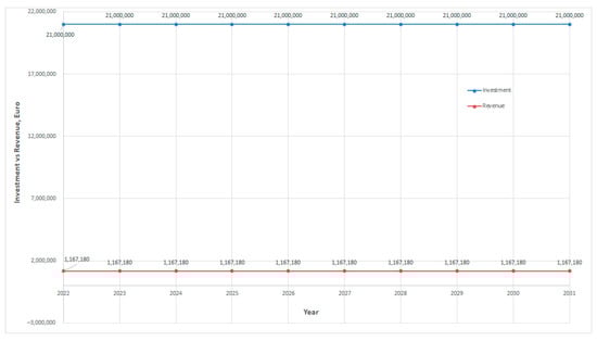
Figure 14.
Volume of investment costs and revenues, EUR—scenario 2 (source: authors based on the analysed data).
Another positive aspect that is easy to highlight is that the revenues are three times higher than the base scenario, marking a significant difference.
5. Discussions, Summary and Conclusions
In general, gas losses are treated statistically, based on the defects identified and the norms that allow for their estimation.
Information on technological losses is used in the gas balance, which is carried out at various intervals. The shorter the time interval, the closer the information on technological losses is to reality. The longest time interval, three months, represents the time between the two measurements of the gas volume consumed by the small consumers, and it is used for a volume correction due to the measurements with equipment without a converter.
Using a balance zone model, the average pressures on the balance zones are accurately determined based on the model, which is reflected in the accuracy of how technological consumption is determined.
The balance on the local M&R stations can give an accurate, daily picture of the customers, the areas that produce imbalances. The problem is that even these values are subject to metrological accepted measurement errors, thus introducing more uncertainties.
The model used for determining the gas losses calibrated experimentally, with experimentally determined flow coefficients, can be used for calculating losses due to the non-conformities in the distribution system.
The results are relevant and the calculations for the technological losses made with the proposed model are sufficiently accurate under the given technological conditions.
Using the produced diagrams, it will be possible to very quickly calculate the flow losses due to the ill-fitting for other pressures than the experimentally analysed ones. Moreover, the calculation can be made both using the coefficients as well as the tabulated values. Extrapolations of the experimental results were also made for pipe diameters of 3″, 4″, 6″, and 8″. Due to the materials, equipment, and technology particularities, these values are justified only for Romanian gas distribution systems.
Considering the tests conducted on the same pipeline with the same type of seam but with the equipment mounted several times, or the joint re-fitted several times, it was observed that it is very important how the equipment mounting is done, because the size of the seam can result in great differences in the gas loss calculation.
The study continued with the development of an application that incorporates both these types of technological losses as well as the actual network data for a dynamic gas balance check on a distribution network. From one balance zone to another, gas usually arrives through the medium pressure network, making it necessary to model the medium pressure network dynamically, in order to close the calculations. The method is limited by the sampling rate of the measured values. Gas losses depend on the local pressure in the distribution network, atmospheric pressure, atmospheric temperature, and the size of the fault.
Based on the correlations between the annual values of M&R, AMR, and the small consumption volume and losses associated with gas rings and network characteristics (No. of valves, regulating points, lengths, and their subcategories), useful correlations were obtained in diagnosing the problem areas and highlighting the proposed measures.
The analysis of the energy balance aimed to: locate the real energy losses, determine their causes and classification, as well as establish the measures to be applied to optimise the techno-economic indicators.
Based on the conclusions of the actual balance analysis, a set of measures was drawn up, including possible technical measures to eliminate or reduce losses.
In order to estimate the environmental impact, the CO2 equivalent was calculated based on the amount of natural gas lost from the system.
The study presents an economic estimate, based on two scenarios, regarding the replacement of pipeline sections in the natural gas networks. Scenario 2 maintains the same conclusion is scenario 1: comparatively, there is a very large difference between the investment volume and the revenue from the reduction in the losses. The main advantages address the environmental protection and the elimination of technological risks with a positive social health impact, for which we stress that these investments are of a strategic importance. Another positive aspect that is easy to highlight is that the values recorded from the revenues are significantly higher; in fact, they are three times higher than the scenarios considered above, even if the investment levels are higher. Additionally, loss diminishing brings a social advantage to the householder’s consumers through a reduction in the gas price.
Author Contributions
Conceptualization, C.N.E., A.N. and D.B.S.; methodology, C.N.E., A.N. and D.B.S.; software, D.B.S. and C.N.E.; validation, C.N.E., A.N. and D.B.S.; formal analysis, D.B.S.; investigation, C.N.E., A.N. and D.B.S.; resources, D.B.S. and C.N.E.; data curation, D.B.S. and C.N.E.; writing—original draft preparation, C.N.E., A.N. and D.B.S.; writing—review and editing, C.N.E., A.N. and D.B.S.; visualization, C.N.E., A.N. and D.B.S.; supervision, C.N.E.; project administration, A.N.; funding acquisition, C.N.E., A.N. and D.B.S. All authors have read and agreed to the published version of the manuscript.
Funding
This research was funded by Petroleum-Gas University of Ploiesti and the APC was funded by CNFIS grant number CNFIS-FDI-2022-0319.
Data Availability Statement
Data is unavailable due to privacy restrictions.
Acknowledgments
This article represents the material of the contract no. 3967/06.04.2021 concluded between DISTRIGAZ SUD RETELE S.R.L. and the Petroleum-Gas University of Ploiesti with the topic Study on the defects of equipment with leaks in the distribution system.
Conflicts of Interest
The authors declare no conflict of interest.
Nomenclature
| p | Natural gas pressure in pipeline [bar] |
| k | Adiabatic exponent |
| T | Gas temperature [K] |
| m | Gas mass [kg] |
| V | Pipeline volume [m3] |
| Z | Non-ideal coefficient |
| τ | Time [s] |
| ANRE | Romanian Energy Regulatory Authority |
| DS | Distribution System |
| DSO | Distribution System Operator |
| M&R | Metering and Regulating Station |
| AMR | Automatic Meter Reading |
| HDPE (PEHD) | High-density polyethylene or polyethylene high-density is a thermo-plastic polymer produced from the monomer ethylene |
References
- Neacsa, A.; Panait, M.; Muresan, J.D.; Voica, M.C.; Manta, O. The Energy Transition between Desideratum and Challenge: Are Cogeneration and Trigeneration the Best Solution? Int. J. Environ. Res. Public Health 2022, 19, 3039. [Google Scholar] [CrossRef] [PubMed]
- Neacsa, A.; Panait, M.; Muresan, J.D.; Voica, M.C. Energy Poverty in European Union: Assessment Difficulties, Effects on the Quality of Life, Mitigation Measures. Some Evidences from Romania. Sustainability 2020, 12, 4036. [Google Scholar] [CrossRef]
- Apostu, S.A.; Panait, M.; Vasile, V. The energy transition in Europe-a solution for net zero carbon? Environ. Sci. Pollut. Res. Int. 2022, 29, 71358–71379. [Google Scholar] [CrossRef] [PubMed]
- Neacsa, A.; Eparu, C.N.; Stoica, D.B. Hydrogen–Natural Gas Blending in Distribution Systems—An Energy, Economic, and Environmental Assessment. Energies 2022, 15, 6143. [Google Scholar] [CrossRef]
- Noja, G.G.; Cristea, M.; Panait, M.; Trif, S.M.; Ponea, C.Ș. The Impact of Energy Innovations and Environmental Performance on the Sustainable Development of the EU Countries in a Globalized Digital Economy. Front. Environ. Sci. 2022, 10, 934404. [Google Scholar] [CrossRef]
- Lustenberger, P.; Schumacher, F.; Spada, M.; Burgherr, P.; Stojadinovic, B. Assessing the Performance of the European Natural Gas Network for Selected Supply Disruption Scenarios Using Open-Source Information. Energies 2019, 12, 4685. [Google Scholar] [CrossRef]
- Moghadam Dezfouli, A.; Saffarian, M.R.; Behbahani-Nejad, M.; Changizian, M. Experimental and numerical investigation on development of a method for measuring the rate of natural gas leakage. J. Nat. Gas Sci. Eng. 2022, 104, 104643. [Google Scholar] [CrossRef]
- Yang, Y.; Fan, J.; Wu, S.; Liu, D.; Ma, F. Multi-acoustic-wave-feature-based method for detection and quantification of downhole tubing leakage. J. Nat. Gas Sci. Eng. 2022, 102, 104582. [Google Scholar] [CrossRef]
- Hormaza Mejia, N.A.; Brouwer, J. Gaseous Fuel Leakage from Natural Gas Infrastructure. In Proceedings of the ASME 2018 International Mechanical Engineering Congress and Exposition, Pittsburgh, PA, USA, 9–15 November 2018. [Google Scholar]
- Hou, Q.M.; Jiao, W.L.; Zou, P.H. The Analysis for the Environmental Impact of Natural Gas Leakage and Diffusion into the Atmosphere. Adv. Mater. Res. 2011, 225–226, 656–659. [Google Scholar] [CrossRef]
- Xu, H.; Sinha, S.K. A Framework for Statistical Analysis of Water Pipeline Field Performance Data. In Pipelines 2019; American Society of Civil Engineers: Reston, VA, USA, 2019; pp. 180–189. [Google Scholar]
- Xu, H. Software Development for Fuzzy Logic-Based Pipe Condition Prediction. In Pipelines 2022: Construction and Rehabilitation; American Society of Civil Engineers: Reston, VA, USA, 2022; pp. 30–40. [Google Scholar]
- Adrian, N.; Alin, D.; Baranowski, P.; Sybilski, K.; Naim, R.I.; Malachowski, J.; Blyukher, B. Experimental and Numerical Testing of Gas Pipeline Subjected to Excavator Elements Interference. J. Press. Vessel. Technol. 2016, 138, 031701. [Google Scholar] [CrossRef]
- Eparu, C. Managementul Sistemelor de Distribuție Gaze Naturale; Editura Universității Petrol-Gaze din Ploiesti: Ploiesti, Romania, 2019. [Google Scholar]
- Eurogas-MARCOGAZ. Emissions Methodology for Estimation of Methane Emissions in the Gas Industry. Final Working Group Report; Joint Group Environment Health and Safety Working Group on Methane, 2003. [Google Scholar]
- MARCOGAZ. Methane Emissions in the Gas Sector. In Proceedings of the GIE, Vienna, Austria, 26–27 November 2019. [Google Scholar]
- Eparu, C.; Neacşu, S.; Stoica, D.B. An Original Method to Calculate the Daily Gas Balance for the Gas Network Distribution. In Proceedings of the 21st International Business Information Management Association (IBIMA) Conference, Vienna, Austria, 27–28 June 2013; pp. 735–747. [Google Scholar]
- Eparu, C.N.; Neacsu, S.; Prundurel, A.P.; Radulescu, R.; Neacșa, A. Behaviour of transmission and distribution networks with big consumption, the stress test. IOP Conf. Ser. Mater. Sci. Eng. 2019, 595, 012010. [Google Scholar] [CrossRef]
- Eparu, C.; Albulescu, M.; Neacsu, S.; Albulescu, C. Gas leaks through corrosion defects of buried gas transmission pipelines. Rev. Chim. 2014, 65, 1385–1390. [Google Scholar]
- EPA. Protocol for Equipment Leak Emission Estimates; EPA: Washington, DC, USA, 1995. [Google Scholar]
- Guvernul_Romaniei. Ordinul nr. 221/2019 Pentru Modificarea Şi Completarea Metodologiei de Calcul al Consumului Tehnologic Din Sistemele de Distribuţie a Gazelor Naturale, Aprobată Prin Ordinul Preşedintelui Autorităţii Naţionale de Reglementare în Domeniul Energiei nr. 18/2014; Guvernul_Romaniei: Bucharest, Romania, 2019. [Google Scholar]
- Guvernul_Romaniei. Ordinul Președintelui ANRE nr. 18/2014 Pentru Aprobarea Metodologiei de Calcul al Consumului Tehnologic Din Sistemele de Distribuție a Gazelor Naturale; Guvernul_Romaniei: Bucharest, Romania, 2014. [Google Scholar]
- ANRE. Available online: www.anre.ro. (accessed on 15 October 2022).
- Eparu, C.N.; Neacsu, S.; Neacsa, A. Correlation of Gas Quality with Hydrodynamic Parameters in Transmission Networks. MATEC Web Conf. 2019, 290, 10001. [Google Scholar] [CrossRef]
- Casson, D.R.; Peters, G.; Nelson, K. Methodology for estimating leakage rates used in the 1992 British Gas national leakage tests. Br. Gas Res. Technol. 1995. [Google Scholar]
- ISI. Methane Emissions Caused by the Use of Gas in Germany between 1990 and 1997 with an Outlook for 2010; Fraunhofer Institut für Systemtechnik und Innovationsforschung (ISI)—Institute of System Engineering & Innovation Research: Karlsruhe, Germany, 2000. [Google Scholar]
- Stoica, D.B.; Eparu, C.N.; Neacsa, A.; Prundurel, A.P.; Simescu, B.N. Investigation of the gas losses in transmission networks. J. Pet. Explor. Prod. Technol. 2021, 12, 1665–1676. [Google Scholar] [CrossRef]
- MARCOGAZ. Survey Methane Emissions for Gas Transmission in Europe; The Technical Association of the European Gas Industry: Brussels, Belgium, 2018. [Google Scholar]
- Neacșu, S.; Eparu, C.; Neacșa, A. The Optimization of Internal Processes from a Screw Compressor with Oil Injection to Increase Performances. Int. J. Heat Technol. 2019, 37, 148–152. [Google Scholar] [CrossRef]
- Neacsa, A.; Rehman Khan, S.A.; Panait, M.; Apostu, S.A. The Transition to Renewable Energy—A Sustainability Issue? In Energy Transition: Economic, Social and Environmental Dimensions; Khan, S.A.R., Panait, M., Puime Guillen, F., Raimi, L., Eds.; Springer Nature Singapore: Singapore, 2022; pp. 29–72. [Google Scholar]
Disclaimer/Publisher’s Note: The statements, opinions and data contained in all publications are solely those of the individual author(s) and contributor(s) and not of MDPI and/or the editor(s). MDPI and/or the editor(s) disclaim responsibility for any injury to people or property resulting from any ideas, methods, instructions or products referred to in the content. |
© 2022 by the authors. Licensee MDPI, Basel, Switzerland. This article is an open access article distributed under the terms and conditions of the Creative Commons Attribution (CC BY) license (https://creativecommons.org/licenses/by/4.0/).