On the Simulations of Thermal Liquid Foams Using Lattice Boltzmann Method

Abstract

Liquid foams exist in a wide variety of chemical and industrial processes, and they can contaminate the end-product and cause time and economical losses. Understanding and simulating foam is not a straightforward task, due to the highly dispersed time and length scales where the physical phenomena occur. Surfactants’ or proteins’ length scales are far beyond the capability of macroscopic and even mesoscopic numerical fluid solvers, yet the macroscales are still required to be resolved. Meanwhile, the lattice Boltzmann method (LBM) has gained much attention and success as a mesoscopic approach which can deal with complex multiphase multicomponent systems. The aim of this study is to implement LBM to simulate liquid foams while considering the accompanying thermal effects. A coupled multiphase multicomponent thermal flow model and its selected add-ons from the literature are tuned and explained, limitations and future suggestions are fairly discussed. Validations and a final study case are shown as an example for the proposed model and its applicability in thermal liquid foams. Finally, a delicate treatment to back couple the effect of temperature on the surface tension is proposed, hence considering one aspect of the Marangoni effect. Initial results show promising behavior, which can be material for future investigations.

1. Introduction

Foams exist in several chemical and industrial processes, and they often delay and obstruct the production. Foam is a complex multiphase multicomponent system, and it often consists of one or more coexisting gas components (air and vapor) in the bubble and liquid phase represented in the lamella (water). The lamellar interfacial length can reach orders of nanometers depending on whether the stabilizing agents are surfactants or proteins [1]. The lamella of protein foams normally have higher length scales than surfactants’ ones [2]. The repulsive forces between the surfactants or protein molecules in the lamellar interface often induce high positive values of disjoining pressure, which is the reason for stable foams [3]. Quantification of these disjoining pressure isotherms is often undertaken by thin film pressure balance technique, where the thickness of the thin film is controlled and measured with the film pressure until reaching the Black Newton film and, hence, rupture [4].

Thermal effects and gradients add more physical complexities to the foam system, such as evaporation–condensation, viscosity variations and the local variation of surface tension, leading to the Marangoni effect [5]. These complex phenomena interact with each other. For example, one of the most foam-dynamics influencing phenomena is the liquid drainage through the lamella [2]. However, temperature variation can highly affect the surface tension, leading to an induced flow, which may be in an unfavorable direction opposing the drainage one, hence leading to more stable foam [6]. There also exists the coarsening or Ostwald ripening in foams, where gas diffuses from smaller bubbles to larger bubbles [1]. This process is normally more important on the larger time scales, when compared to the drainage and convective mass flow.

Modelling and simulation of these interacting processes are not straightforward, although some aspects can be tackled using the mesoscopic lattice Boltzmann method (LBM), which has proven its capability of modelling complex multiphase and thermal flows [7]. The idea of the current work is to propose an approach to simulate some of these phenomena and discuss the current limitations based on the literature and current experience.

For the multiphase models in LBM, the two most famous methods are the free-energy [8,9] and the pseudopotential Shan-Chen (SC) [10,11] approaches. The limitation of the high density ratio and viscosity ratios are always issues for both methods. The adopted approach in this work is the SC model, since it is possible to extend it to approach the simulation of liquid foams by reaching positive values of disjoining pressure. The original SC model can also reach higher stable density ratios up to 100 and can be extended to reach ratios up to 1000, though with a modified equations of state (EOS). In the work by Yuan and Schaefer [12], they studied several equations of state, where Peng-Robinson (P-R) EOS [13] yielded the highest stable density ratio and the least spurious currents, which is a well-known issue in multiphase models. The higher viscosity ratios issue can generally be stabilized by switching from the standard LBM single relaxation time (SRT) collision operator to either the two or multiple relaxation time (TRT or MRT) [14]. SC model can also reach comparable and even slightly higher surface tensions than the free-energy approach [14].

There also exists the free-surface (FS) LBM approach, where the dense component is considered while the other one is neglected; this somehow resembles the Volume of Fluid (VOF) approach in LBM. In the work by Körner et al. [15] and later by Ataei et al. [16], much success has been gained with reaching stable foam by introducing linearly variable repulsive forces as a function of the lamellar distance. Interfacial curvature estimation [17] is required for the FS-LBM in general, in addition to ray tracing algorithms for the lamellar distance evaluation. Nevertheless, the presented work is mainly focused on the SC LBM approach, where neither the tracking nor the curvature estimation is required, not to mention the lamellar distance evaluation.

The SC LBM is based on modelling the molecular interaction between phases and components to reach the phase separation “bottom-up approach” [18]. The original SC can be extended to model both multiphase and multicomponent system, while being able to tune the density ratio and surface tension separately [19]. In order to simulate foams, the surfactants effects shall be implemented into these interaction forces. This can be carried out by using the mid-range interaction (repulsion) in addition to the short-range one [20,21]. This benefit emerges from the nature of the SC LBM, modeling the molecular interactions themselves. This can lead to a positive disjoining pressure, hence delaying bubbles coalescence and obtaining foam! It is worth mentioning that even using a mesoscale method such as LBM, it is practically impossible to resolve the length scales of surfactants molecules; that is why only their forces’ effects are modelled.

In the literature, there also exists the model presented by Chen et al. [22] and Nekovee et al. [23], which is based on introducing two extra sets of LBM distribution functions in addition to the SC LBM system, representing the surfactants species (position) and their own dipolar orientation, although, in the current work, we preferred avoiding this approach for foam simulations for three reasons. First, the model adds much more complexity to the already saturated system of LBM distribution functions. Second, relating the relaxation time, hence the diffusivity of the surfactants position and orientation, to the physical ones could not be seen to be possible. On the other hand, in the mid-range interaction model, the resulting disjoining pressure can be evaluated and, hence, there might be a way to relate it to the experimental isotherms. Third, it is reported in the work from Mukherjee et al. [24] that the model by itself could not inhibit the bubbles coalescence.

Thermal phase change from liquid to gas and vice versa using LBM has been proposed by Gong and Cheng [25] and further enhanced by Li et al. [26]. The model is based on coupling the temperature field by including a source term responsible for the enthalpy of phase change with the SC multiphase model, which is modified by the temperature dependent P-R EOS. However, in addition to the stability issues which are encountered, maintaining both the thermodynamic consistency for phase change and obtaining positive disjoining pressure, which is an essential property of foam formation and stability, has to our knowledge not been developed in the literature.

In the literature, the Enthalpy-based LBM to model phase change for liquid to solid states also exists [27,28], which might be a compromise to investigate the phase change in extremely stable foam by only tracking the interface front between liquid and gas phases accordingly with the temperature field.

The current work aims to propose a recipe for model combination in the scope of SC LBM, in order to simulate the thermal effects in liquid foam without taking into account the phases change. The convective diffusive heat transfer and thermal effects consideration while simulating the flow field in liquid foam is the key innovation in this work. Coarsening or Ostwald ripening will not be discussed in this work, since controlling the mass diffusivity of gas in liquids using the SC model separately is numerically impossible.

The paper is arranged as follows: the LBM and SC model are briefly proposed, showing the multiphase–multicomponent simulation parameters, the implemented forcing scheme and the TRT. The mid-range interaction model is proposed and explained. The temperature field and how it is implemented is shown. Units and non-dimensional groups to change from lattice to physical units are discussed. For the following section, a model verification is carried out by relating the interaction numerical parameters to the physical ones through the Young–Laplace test, where surface tension and density ratio (using SC EOS) are tuned and evaluated for different bubble sizes. Rayleigh–Taylor instability (RTI) is shown as a validation case for the implemented multiphase–multicomponent model and compared with numerical test cases from the literature. Simulation samples from the bubble rise diagram by Clift et al. [29] are presented in brief as a further qualitative validation for different Reynolds and bonds numbers, showing the model capability of capturing the interfacial behavior for different bubble regimes. In the application section, the developed model is applied for a case study of one-way coupled heat transfer in dynamic liquid foam while using the mid-range interaction model. Finally, a new technique to consider the variable surface tension due to temperature gradients is proposed, hence suggesting a technique to account for the Marangoni effect in thermal foams using SC LBM. A summary and conclusion section is shown to finalize the whole presented model, discuss the achievement fairly and suggest future work in order to reach the final aim of simulating the foam in industrial scale processes.

2. Materials and Methods

2.1. Lattice Boltzmann Method

The lattice Boltzmann method is based on the well-known Boltzmann Equation, where particles’ motion and interaction in space and time are represented by the particle distribution function $f$, as shown in Equation (1) [30].

$$\frac{\partial f}{\partial t}+\widehat{\mathit{v}}\cdot \nabla f=Q$$

(1)

where $t, \widehat{\mathit{v}}$ and $Q$ are time, particle microscopic velocity and the collision operator. $Q$ is originally found in a complex integral form which can be approximated using the Bhatnagar–Gross–Krook (BGK) relaxation, namely the single relaxation time (SRT) [31]. It represents the particles’ relaxation from non-equilibrium to the local equilibrium state during collision, through the time $\tau$ as shown in Equation (2) [30], where the equilibrium distribution function $f^{equ}$ can be formulated in the scope of the kinetic theory of gases using the Maxwell–Boltzmann distribution.

$$Q=-\frac{1}{\tau }\left[f-f^{equ}\right]$$

(2)

Discretizing the particle distribution function into a subspace of discrete lattice velocities $i$, mimicking the degrees of freedom of where the particles can propagate in space, the distribution function can be shown as $f_i(\widehat{\mathit{x}},t)$. This can be explained as the probability of finding a particle in position vector $\widehat{\mathit{x}}$ at time $t$ with a microscopic speed in the direction $i$, using the explicit time integration, which when based on the trapezoidal rule [32] maintains the second order accuracy of the LBM in time [14]. The lattice Boltzmann equation (LBE) finally reads as:

$$f_i(\widehat{\mathit{x}}+{\widehat{\mathit{e}}}_i\Delta t,t+\Delta t)=f_i(\widehat{\mathit{x}},t)-\frac{1}{\tau }\left(f_i(\widehat{\mathit{x}},t)-f_i{}^{equ}(\widehat{\mathit{x}},t)\right)$$

(3)

The above equation carries the core procedure of the LBM, showing the propagation of particles from one lattice position to the other and the collision operation, i.e., relaxation [33]. The equilibrium distribution function is based on the Hermite series expansion of the Maxwell–Boltzmann distribution with the truncation up to the second order macroscopic velocity, which is valid for low lattice Mach numbers and can be written as:

$$f_i{}^{equ}=w_i\rho \left[1+3\frac{{\widehat{\mathit{e}}}_i\cdot \widehat{\mathit{u}}}{c^2}+\frac{9}{2}\frac{{({\widehat{\mathit{e}}}_i\cdot \widehat{\mathit{u}})}^2}{c^4}-\frac{3}{2}\frac{\widehat{\mathit{u}}\cdot \widehat{\mathit{u}}}{c^2}\right]$$

(4)

where ${\widehat{\mathit{e}}}_i$, $w_i$, $c$, $\rho$ and $\widehat{\mathit{u}}$ are the lattice unit vectors, weighting parameter, lattice speed (lattice spacing/lattice time step size $\Delta x/\Delta t=1$), macroscopic density and velocity, respectively.

The macroscopic density and velocity can be evaluated from the 0th and 1st moment of the distribution function, respectively, as follows:

$$\rho ={\displaystyle \sum _{i=0}^8{f}_i} ; \widehat{\mathit{u}}=\frac{1}{\rho }{\displaystyle \sum _{i=0}^8{f}_i{\widehat{\mathit{e}}}_i}$$

(5)

The common D2Q9 is used here representing a 2D case and 9 lattice directions. The weighting parameters for the D2Q9 according to the short-range interaction from Figure 1 (presented in red) are listed in

Table 1. Weighting parameter $w_i$ values for the D2Q9 lattice.

$\mathbf{Direction} {\widehat{\mathit{e}}}_{\mathit{i}}$	${\mathit{w}}_{\mathit{i}}$
0	4/9
1, 2, 3, 4	1/9
5, 6, 7, 8	1/36

. Although LBM in accordance with the SC model (Section 2.2) is easily represented in 3D, the interest in this work is limited to the 2D case. Taking into consideration that the 2D mid-range interaction model (Section 2.5) requires the information from 24 neighboring nodes, the 3D case would require 92 in order to maintain the same 8th order of isotropy [21], which means much higher computational cost.

The LBM relaxation time can be related to the fluid kinematic viscosity through the Chapman–Enskog expansion, and comparing it with the incompressible Navier–Stokes equation leads to the following equation:

$${\tau }_{}=3{\mathit{v}}_{LU}+0.5$$

(6)

where $v_{LU}$ stands for the kinematic viscosity in lattice unis (LU). The Mach number $M$, lattice speed of sound $c_s$ and static pressure $p$ based on the isothermal ideal equation of state can be presented, respectively, as follows:

$$M=\frac{\Vert \widehat{\mathit{u}}\Vert }{c_s}, c_s=\frac{c}{\sqrt{3}}, p=\rho c_s{}^2$$

(7)

2.2. Shan-Chen Multiphase Multicomponent Model

The main benefit of the Shan-Chen [10,11] multiphase multicomponent model is that it does not dictate tracking any interface, since the separation automatically occurs due to the repulsive and attraction forces between components and phases, respectively. The SC is a pseudopotential method based on the potential function $\psi$ as shown in Equation (8), which leads to the non-ideal equation of state as shown in Equation (9). The potential function can be written in two cases, and case A is reported to be more stable than case B [19] although case B will be used in a specific case as explained in Section 2.5.

$${\psi }^{(\sigma )}=\{\begin{array}{c}{\rho }_o\left[1-e^{\frac{-{\rho }^{(\sigma )}}{{\rho }_o}}\right]\\ {\rho }^{(\sigma )}\end{array} \begin{array}{c}case A\\ case B\end{array}$$

(8)

$$p=c_s{}^2{\displaystyle \sum _{\sigma }\left({\rho }^{(\sigma )}+\frac{1}{2}{G}_{\sigma \sigma } {\psi }^{(\sigma )}{}^{{}^2}\right)+}\frac{c_s{}^2}{2}{\displaystyle \sum _{\sigma , \tilde{\sigma }}{G}_{\sigma \tilde{\sigma }} {\psi }^{(\sigma )} }{\psi }^{(\tilde{\sigma })}$$

(9)

where ${\rho }_o$, $\sigma$, $\tilde{\sigma }$ and $G$ represent the reference density which is taken as unity, the respected component, opposite components indices and the interaction parameter between phases and components, respectively. Here, both the interaction between phases and components are included. Only two components are considered in this work, 1 and 2. Setting the value of $G_{11}=0$, $G_{12}=G_{21}>0$, and $G_{22}<0$ will lead to the presence of the two components with the coexistence of the component 2 in both phases. Tuning the two non-zero parameters will lead to controlling both the density ratio and surface tension separately.

The local SC interaction force for each component with respect to the neighboring nodes will then be presented as:

$${\widehat{\mathit{F}}}_{SC}{}^{(\sigma )}(\widehat{\mathit{x}})=- {\psi }^{(\sigma )}(\widehat{\mathit{x}}) \left(G_{\sigma \tilde{\sigma }}{\displaystyle \sum _{i=0}^8{w}_i {\psi }^{(\tilde{\sigma })}(\widehat{\mathit{x}}+c_i\Delta t) {\widehat{\mathit{e}}}_i} + G_{\sigma \sigma }{\displaystyle \sum _{i=0}^8{w}_i {\psi }^{(\sigma )}(\widehat{\mathit{x}}+c_i\Delta t) {\widehat{\mathit{e}}}_i}\right)$$

(10)

For the short range interactions, the potential function $\psi (x+c_i\Delta t)$ requires the density information from the first level of neighbors, which are 8 for the case of D2Q9.

Two LBE are then required for both components with two sets of distribution functions, which can be written as:

$$f_i{}^{ (\sigma )}(\widehat{\mathit{x}}+{\widehat{\mathit{e}}}_i\Delta t, t+\Delta t)=f^{ (\sigma )}{}_i(\widehat{\mathit{x}},t)-\frac{1}{{\tau }^{(\sigma )}}\left(f_i{}^{ (\sigma )}(\widehat{\mathit{x}},t)-f_i{{}^{equ}}^{{}^{(\sigma )}}(\widehat{\mathit{x}},t)\right)+S_i{}^{(\sigma )}(\widehat{\mathit{x}},t)$$

(11)

where $S_i{}^{(\sigma )}(\widehat{\mathit{x}},t)$ is a source term that incorporates the interaction and any other external forces based on the selected forcing scheme shown in Section 2.3, while ${\tau }^{(\sigma )}$ is responsible for the kinematic viscosity of each component. The equilibrium distribution function for each component can be written as:

$$f_i{{}^{equ}}^{{}^{(\sigma )}}=w_i{\rho }^{(\sigma )}\left[1+3\frac{{\widehat{\mathit{e}}}_i\cdot {\widehat{\mathit{u}}}^{\mathbf{\prime }}}{c^2}+\frac{9}{2}\frac{{({\widehat{\mathit{e}}}_i\cdot {\widehat{\mathit{u}}}^{\mathbf{\prime }})}^2}{c^4}-\frac{3}{2}\frac{{\widehat{\mathit{u}}}^{\mathbf{\prime }}\cdot {\widehat{\mathit{u}}}^{\mathbf{\prime }}}{c^2}\right]$$

(12)

where ${\rho }^{(\sigma )}$ and ${\widehat{\mathit{u}}}^{\mathbf{\prime }}$ are the density of each component evaluated as ${\rho }^{(\sigma )}={\displaystyle \sum _{i=0}^8{f}_i{}^{(\sigma )}}$ and the corrected macroscopic velocity of the mixture, which is shown in Equation in 14 in Section 2.3.

2.3. Forcing Scheme

The adopted forcing scheme is the one by Guo et al. [34], as it gave the most stable simulations, lowest interfacial spurious currents and, hence, the highest stable interaction parameter when compared to the simple method by Buick and Greated [35] or the velocity shifting method, which was adopted in the original SC model [10,11]. The scheme by Guo et al. [34] is originally evaluated while considering the discrete lattice effects in order to recover the macroscopic continuity and momentum with external force. It was also reported by Yu and Fan [36] that the model by Guo can produce a $\tau$-independent (viscosity independent) surface tension.

The evaluation of the source term can be written in the terms of the SC interaction force as follows:

$$S_i{}^{(\sigma )}=\left(1-\frac{1}{2 {\tau }^{(\sigma )}}\right) R_i{}^{(\sigma )}; R_i{}^{(\sigma )}=\frac{w_i}{c_s{}^2} \left(F_{S{C}_{{}_{\alpha }}}{}^{(\sigma )} e_{i\alpha }+\frac{e_{i\alpha }{e}_{i\beta }-c_s{}^2{\delta }_{\alpha \beta }}{c_s{}^2}{F}_{S{C}_{{}_{\alpha }}}{}^{(\sigma )} u^{\prime }\beta \right)$$

(13)

where $\alpha$, $\beta$ = 1, 2 for the 2D case, while the corrected macroscopic velocity of the mixture ${\widehat{\mathit{u}}}^{\mathbf{\prime }}$ shall written as a function of the interaction (or any external forces) as follows:

$${\widehat{\mathit{u}}}^{\mathbf{\prime }} =\frac{1}{\rho }{\displaystyle \sum _{\sigma }\left({\displaystyle \sum _{i=0}^8{f}_i{}^{(\sigma )}{\widehat{\mathit{e}}}_i}+\frac{{\widehat{F}}_{SC}{}^{(\sigma )}}{2}\right) }; \rho ={\displaystyle \sum _{\sigma }{\rho }^{(\sigma )}}$$

(14)

Any external gravity or wall forces can be also added directly to the SC interaction forces.

2.4. Two Relaxation Time

Two phase flows always suffer from instabilities, especially when reaching the limiting cases of interaction parameters which are essential in order to tune density ratio and the surface tension together. Additionally, high viscosity ratio is a very high source of instability. This will always lead to the two relaxation time (TRT), which gives an extra degree of freedom for the simulations, yet in a simple way. This is available by splitting the distribution functions to symmetric $f_i{}^{ {(\sigma )}^{ +}}=\left(f_i{ }^{(\sigma )}+f_{-i}{}^{(\sigma )}\right)/2$ and asymmetric parts $f_i{}^{ {(\sigma )}^{ -}}=\left(f_i{ }^{(\sigma )}-f_{-i}{}^{(\sigma )}\right)/2$, where $-i$ stands for the opposite lattice velocity direction. Each of the new distribution functions is relaxed with two separated relaxation times ${\tau }^{(\sigma )}{}^{{}^{+}}$ and ${\tau }^{(\sigma )}{}^{{}^{-}}$, and controlled through the magic parameter $\Lambda$, as shown in Equation (15). It is reported that the value of $\Lambda =1/4$ provides the highest stability [14].

$$\Lambda =\left({\tau }^{{(\sigma )}^{+}}-0.5\right)\left({\tau }^{{(\sigma )}^{-}}-0.5\right); {\tau }^{{(\sigma )}^{ +}}=3{\mathit{v}}_{LU}{}^{(\sigma )}+0.5$$

(15)

while the source term according to Guo et al. [34] shall also be modified as follows [37,38]:

$${S_i{}^{ (\sigma )}}_{TRT}=\left(1-\frac{1}{2{\tau }^{{(\sigma )}^{+}}}\right)R_i{}^{ {(\sigma )}^{ +}}+\left(1-\frac{1}{2{\tau }^{{(\sigma )}^{ -}}}\right)R_i{}^{ {(\sigma )}^{ -}}$$

(16)

where $R_i{}^{ {(\sigma )}^{ +}}=\left(R_i{ }^{(\sigma )}+R_{-i}{}^{(\sigma )}\right)/2$ and $R_i{}^{ {(\sigma )}^{ -}}=\left(R_i{}^{ (\sigma )}-R_{-i}{}^{(\sigma )}\right)/2$ following same idea of splitting the distribution functions. Apart from the collision and forcing steps, the algorithm is exactly the same as the SRT.

2.5. Mid-Range Interaction Model

A positive value of disjoining pressure $\Pi$ is a major macroscopic property of stable thin films, due to the existence of repulsive forces between protein or surfactant molecules [3]. The disjoining pressure can be related to the film tension ${\gamma }^f$ as follows:

$${\gamma }^f=2\gamma -{\displaystyle \underset{\infty }{\overset{l}{\int }}\Pi dl}+\Pi l$$

(17)

where $\gamma$ and $l$ are the surface tension and the film thickness, respectively.

The D2Q25 model is used in order to reach positive values of disjoining pressure, hence stable films and foam [20,21]. The neighboring nodes, far till $\sqrt{8}$ from the central one, are considered as represented in Figure 1 (both red and blue colors). This will yield to a new interaction parameter responsible for the repulsive forces between the same component, which can be called ${\tilde{G}}_{11}={\tilde{G}}_{22}>0$. The extra SC force shall be added to Equation (10), and can be written as:

$${\widehat{\tilde{\mathit{F}}}}_{SC}{}^{(\sigma )}(\widehat{\mathit{x}})=- {\psi }^{(\sigma )}(\widehat{\mathit{x}}){\tilde{G}}_{\sigma \sigma }{\displaystyle \sum _{\tilde{i}=0}^{24}{\tilde{w}}_{ \tilde{i}} {\psi }^{(\sigma )}(\widehat{\mathit{x}}+c_{ \tilde{i}}\Delta t) {\widehat{\mathit{e}}}_{\tilde{i}}}$$

(18)

where ${\widehat{\mathit{e}}}_{\tilde{i}}$ and ${\tilde{w}}_{ \tilde{i}}$ represent the mid-range lattice unit vectors and the weighting parameter as shown in

Table 2. Weighting parameter ${\tilde{w}}_{ \tilde{i}}$ values for the D2Q25 lattice.

$\mathbf{Direction} {\widehat{\mathit{e}}}_{\tilde{\mathit{i}}}$	${\tilde{\mathit{w}}}_{ \tilde{\mathit{i}}}$
0	247/420
1, 2, 3, 4	4/63
5, 6, 7, 8	4/135
9, 10, 11, 12	1/180
13, 14, …, 20	2/945
21, 22, 23, 24	1/15,120

.

The full non-ideal static pressure (EOS) shall then be modified using the scope of Equation (9) as follows:

$$p=c_s{}^2{\displaystyle \sum _{\sigma }\left({\rho }^{(\sigma )}+\frac{1}{2}\left(G_{\sigma \sigma }+ {\tilde{G}}_{\sigma \sigma }\right) {\psi }^{(\sigma )}{}^{{}^2}\right)+}\frac{c_s{}^2}{2}{\displaystyle \sum _{\sigma , \tilde{\sigma }}{G}_{\sigma \tilde{\sigma }} {\psi }^{(\sigma )} }{\psi }^{(\tilde{\sigma })}$$

(19)

2.6. Thermal Field

Temperature field can be added in LBM as a third set of the distribution function, in addition to the two from the two fluid components. The LBE for the temperature distribution function $h_i(\widehat{\mathit{x}},t)$ can be written following the laws of diffusion and convection as follows:

$$h_i(\widehat{\mathit{x}}+{\widehat{\mathit{e}}}_i\Delta t,t+\Delta t)=h_i(\widehat{\mathit{x}},t)-\frac{1}{{\tau }_T}\left(h_i(\widehat{\mathit{x}},t)-h_i{}^{equ}(\widehat{\mathit{x}},t)\right)$$

(20)

where ${\tau }_T$ and $h_i{}^{equ}(\widehat{\mathit{x}},t)$ are the temperature relaxation time and the equilibrium temperature distribution function. Both can be written as follows:

$${\tau }_T=3{\alpha }_{LU}+0.5$$

(21)

$$h_i{}^{equ}(\widehat{\mathit{x}}, t)=w_{i}T\left[1+3\frac{{\widehat{\mathit{e}}}_i\cdot {\widehat{\mathit{u}}}^{\mathbf{\prime }}}{c^2}\right]$$

(22)

where ${\alpha }_{LU}$, $T$ and ${\widehat{\mathit{u}}}^{\mathbf{\prime }}$ are thermal diffusivity in lattice units, the macroscopic temperature evaluated from the zeroth moment of the temperature distribution function ($T={\displaystyle \sum _{i=0}^8{h}_i}$) and the macroscopic mixture velocity imported from the flow field, respectively. It is reported in the work by Guo et al. [39] that truncating the equilibrium temperature distribution function after the first order velocity term still recovers the convective diffusive temperature equation. Although it is a common practice to use a lower resolution lattice for the temperature field (e.g., D2Q4) than for the flow field [39], in the current work the typical D2Q9 as for the flow field is used for the three sets of distribution functions.

Originally, this can be seen as a one-way coupled temperature field with the flow one, although the relation to the surface tension can be locally back-coupled using a locally variable interaction parameter, and will be shown in Section 4.2.

It is worth mentioning that the implementation of the TRT is only essential for the flow field, while for the temperature field SRT is sufficient since the stability issue is not critical. If TRT was to be used, the asymmetric part of the relaxation time would be the one responsible for the thermal diffusion, not the symmetric one as in the kinematic viscosity case according to the scope of Equation (15).

2.7. Units and Non-Dimensional Groups

In order to maintain the physical similarity between the numerical simulations in lattice units, the following non-dimensional groups shall be introduced:

• Reynolds Number:

$$\mathrm{Re}=\frac{\sqrt{gL}L}{v}$$

(23)

where $g$ and $L$ are the gravity and the characteristic length, respectively. Characteristic length will be considered as the domain width or bubble diameter depending on the study case.

2.

Atwood Number:

$$\mathrm{At}=\frac{{{\rho }_l|}_2-{\rho |}_1}{{{\rho }_l|}_2+{\rho |}_1}$$

(24)

where ${{\rho }_l|}_2$ and ${\rho |}_1$ are the liquid phase of the high density component 2 and the low density component 1. It is worth mentioning that, for the short-range interactions, the Atwood number (density ratio) main controller is the interaction parameter $G_{22}$.

3.

Bonds Number:

$$\mathrm{Bo}=\frac{\rho g{L}^2}{\gamma }$$

(25)

where $\rho g$ and $\gamma$ represent the force field applied on the fluid component and the surface tension, whose evaluation with respect to the SC LBM will be discussed in Section 3.1, respectively. It is worth mentioning that, for the short-range interactions, the surface tension main controller is the interaction parameter $G_{12}=G_{21}$.

4.

Prandtl Number:

To relate the flow and the thermal relaxation times, the Prandtl number shall be introduced for the two fluid components, as follows:

$$\mathrm{Pr}=\frac{v}{\alpha }$$

(26)

3. Model Verification and Validation

3.1. Young–Laplace Test

In order to adjust the surface tension with the SC interaction parameters $G$, hence making the connection between the numerical interaction forces and the physical macroscopic property, the Young–Laplace test is always used as a key for model verification. A liquid or gas bubble is initiated in a fully periodic computational domain with a reasonable density for both components accordingly with the chosen interaction parameters. The bubble is then left to reach the steady state, the pressure inside and outside the bubble are evaluated according to Equation (9) or (19), bubble diameter (radius) is measured and the 2D surface tension can be evaluated according to the Young–Laplace equation as follows:

$$\Delta p=p_{inner}-p_{outer}= \frac{\gamma }{R}$$

(27)

where $p_{inner}$, $p_{outer}$ and $R$ are the inner and outer static pressure and bubble diameter, respectively. The adopted criteria to estimate the interface was half the density of the heavier component liquid phase.

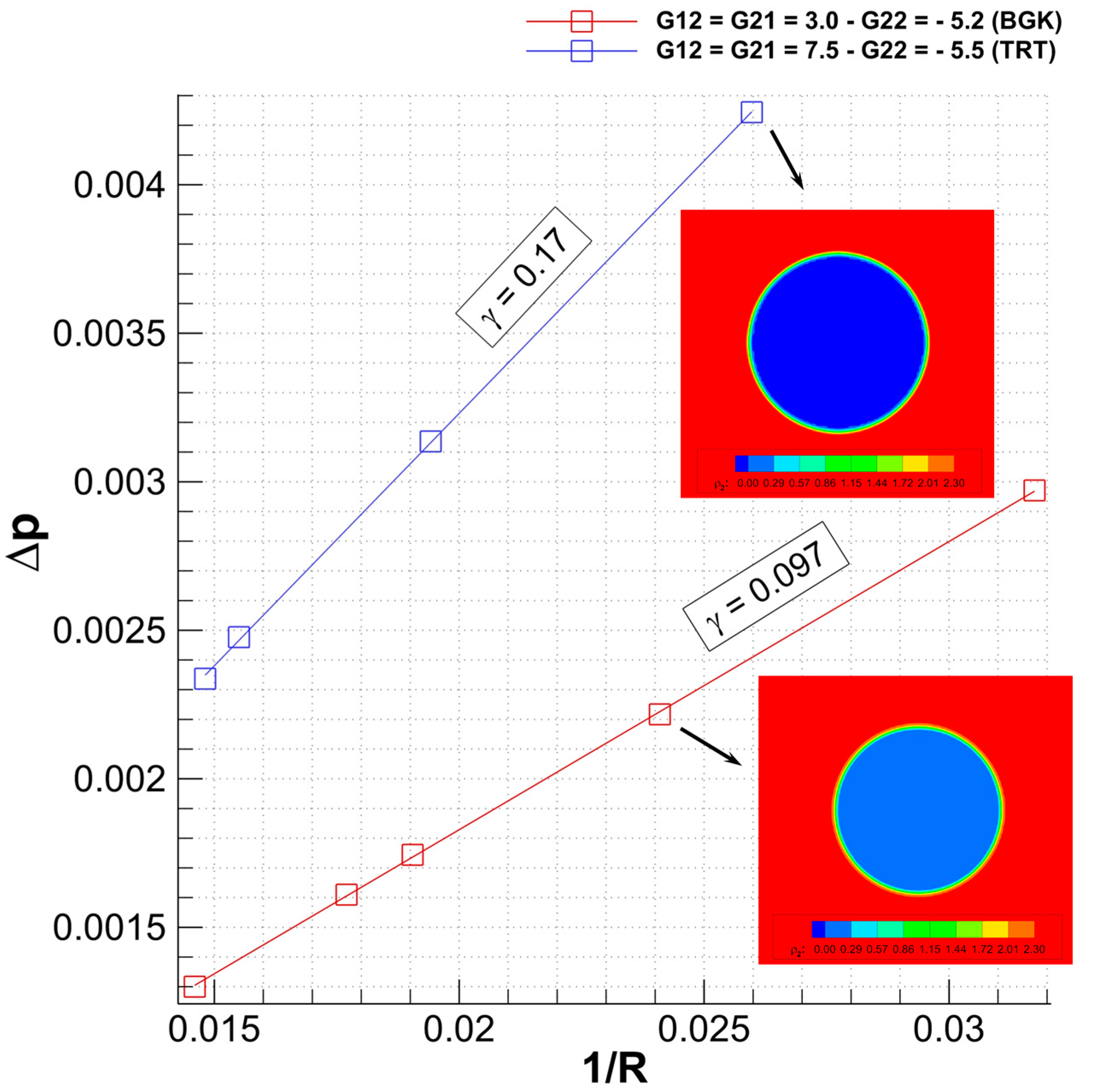
The common procedure is to perform several tests for each combination of interaction parameters and evaluate the surface tension according to the linear regression of the Laplace pressure $\Delta p$ and $1/R$. Figure 2 shows two values of interaction parameters for single phase-two components with density ratio = 1. The two lines represent the two limiting cases: separation between components and numerical stability. The chosen interaction parameters equivalent to the resulting surface tensions in LU are shown on the figure legends. Figure 3 also shows the two limiting cases of surface tension for a two phase two component system with density ratio ≈ 10 between the liquid phase of the high density component 2 and the low density component 1 ($\mathrm{At}\approx 0.8$). The chosen combination of interaction parameters which led to the resulting density ratio and surface tension in LU are shown on the legend. For the higher surface tension case in Figure 3, due to a stability issues, TRT with magic parameter $\Lambda = 1/4$ was required.

For both Figure 2 and Figure 3, the cases of lower surface tension show a non-zero density inside the bubble and a higher interfacial thickness. This is an inherent behavior of the SC model, since it is a diffuse interface approach and does not offer perfectly immiscible components [14]. Density contours in LU are shown for the four Young–Laplace test samples.

3.2. Rayleigh–Taylor Instability

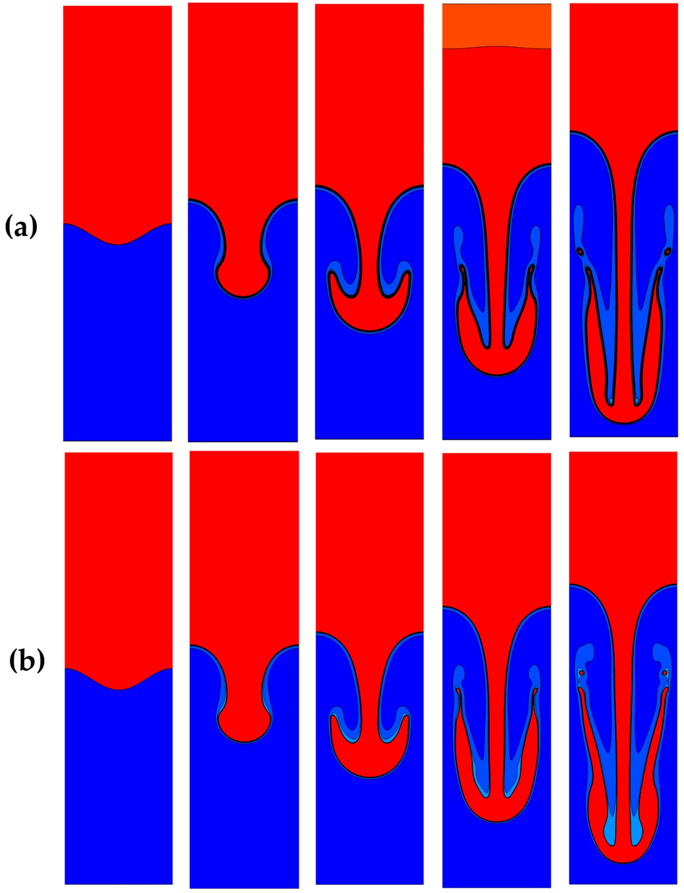
As a model validation, Rayleigh–Taylor Instability is investigated for two different resolutions: 256 × 1024 and 1024 × 4096. As shown in Figure 4, the computational domain consists of a heavier liquid on top impinging the bottom lighter one, with an initial single mode wave of an amplitude of 10% of the domain width. Vertical boundaries are set as periodic. The upper and lower boundaries are set as no-slip walls. Reynolds, Atwood and Bonds numbers are set as 256, 0.5 and 100, respectively. The model shows fair qualitative agreement with the work by He et al. [40] and Chiappini et al. [41]. It is worth mentioning that the surface tension was neglected in both of their works and, therefore, the Bonds numbers are not similar for all cases. Nevertheless, the Bonds number in the shown simulations is fixed for both domain resolutions. The two cases show good mesh independency except for the last time stamp, which is as issue reported and also encountered by [40,41] for both low and high Reynolds numbers, although the last time stamp of the low-resolution case is close to the one from [41], except that the bubble separation appeared slightly before our presented case.

The selected SC interaction parameters for reaching the required density ratio and surface tension are: $G_{12}=G_{21}=3.15$, $G_{22}=-3.4$ and $G_{22}=-3.4$. The kinematic viscosities of both components are kept the same (${\mathit{v}}_{component 1}={\mathit{v}}_{component 2}$). The adopted wall boundary condition is based on the extrapolation scheme by Chen et al. [42], where ghost nodes are introduced behind the boundaries and unknown distribution functions are extrapolated from the inner fluid nodes. Other boundary treatments, such as the non-equilibrium extrapolation method from Guo et al. [43], showed less stability and sudden phase changes close to the walls, which is why it was avoided in the current work. Other types of boundary treatments could be material for future investigations.

3.3. Bubble Rise Diagram

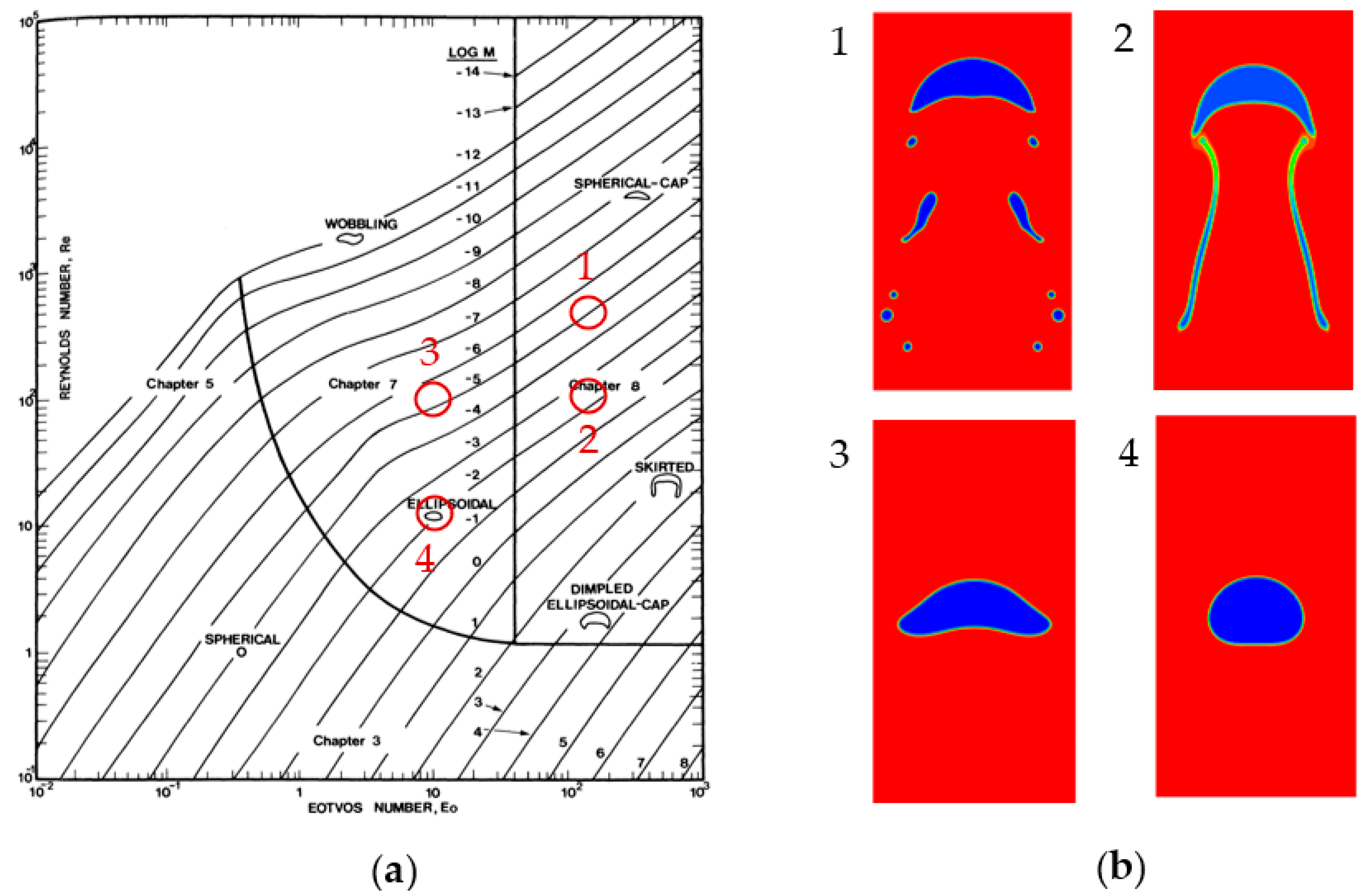
Some samples from the well-known bubble rise diagram by Clift et al. [29] were numerically investigated in order to qualitatively validate the presented SC LBM model for different Reynolds and Bonds numbers. Periodic boundary condition is set on the domain’s edges, while selected time stamps from each case are shown in Figure 5. The Atwood number is set as zero, while the SC interaction parameters are $G_{12}=G_{21}=6.0$ and $G_{11}=G_{22}=0$. The selected points have the following Bonds and Reynolds numbers:

• Bo = 100, Re = 500
• Bo = 100, Re = 100
• Bo = 10, Re = 100
• Bo = 10, Re = 10

The results have very good qualitative agreement with the shape regimes for bubble rise, showing the complex interfacial deformation behaviors. In Case 1, with the highest Reynolds and Bonds number, edges of the bubble are quickly split to smaller bubbles and only the cap remains. In Case 2, with lower Reynolds number, the bubble skirts and the splitting is less severe. In Case 3, with lower Bonds number, the bubble is connected, though it starts wobbling along its motion. In Case 4, with the lowest Reynolds and Bonds number, the bubble shows a slight spherical shape.

All the simulations in this section were carried out using the TRT with $\Lambda =1/4$ for stability issues that occurred with SRT at high Reynolds and Bonds numbers. It is Worth mentioning that the Reynolds number in this simulation is based on $\sqrt{2gR}$ according to Equation (23) instead of the terminal velocity as in [29], which will yield to ~5% difference between both Reynolds numbers according to the terminal velocity formula by Davis and Taylor [44].

4. Application

4.1. Thermal Field in Liquid Foam

For the study case of thermal foam, randomly generated bubbles are initiated at the bottom of a partially filled flask-like domain and left to rise due to the gravitational effect (buoyancy) as shown in Figure 6. No slip boundary condition is set on the four walls. The thermal field model is implemented, where Dirichlet boundary condition is set for the three and bottom (source) walls. All the simulation parameters are shown in

Table 3. Simulation parameters for the thermal foam case study.

Simulation Parameter	Value
Resolution	1000 × 1000
Re	10
Bo	0.1
${\mathrm{Pr}}_{\mathit{component} 1}$	0.72
${\mathrm{Pr}}_{\mathit{component} 2}$	6.0
G12 = G21	5.45
G11 = G22	−2.0
${\tilde{G}}_{11}={\tilde{G}}_{22}$	5.0
θ *	20˚
$T_{\mathit{source}}/T_{\mathit{ref}}$	1.0
$T_{\mathit{walls}}/T_{\mathit{ref}}$	0.25
$R_{initial}$	20 LU
${\mathit{v}}_{\mathit{component} 1}={\mathit{v}}_{\mathit{component} 2}$	-

*: Cone angle.

. The D2Q25 interaction model is implemented to obtain stable foam, while the SC potential function for the interaction between the two components are set using the case B from Equation (8), following the scope of work by Dollet et al. [45] and Fei et al. [46], as it provided much higher bubble stability than case A. For the other two same-component interactions, case B is still used. The surface tension is re-estimated for this case following the same procedure as in Section 3.1, to evaluate the Bonds number. Although the interaction parameters presented by Fei et al. [46] to reach the highest positive disjoining pressure were $G_{12}=G_{21}=3.0$, $G_{11}=G_{22}=-8.0$ and ${\tilde{G}}_{{}_{11}}={\tilde{G}}_{{}_{22}}=7.0$, the required repulsive forces for this bubble rising case between the same components seemed to be higher than the attraction ones in order to maintain stable bubbles.

The simulation time evolution shows the generation of foam layers from rising bubbles as shown in the figure. Before imposing the bubbles’ flow, a pre-time loop is used to reach the steady state for the thermal field. A one-way coupled temperature field is also shown, where the thermal convection due to the bubbles’ motion and rearrangement in the lamella is clearly visible. Thermal diffusion inside bubbles is shown to be much slower than in the liquid due to the different Prandtl number. It is not possible to reach this kind of stable foam using solely the short-range interaction model. The bubbles’ deformation without or with much delayed coalescence, either with the upper interface or between bubbles themselves, are obvious through the shown interfaces. Contact angle is not considered in this work, which will affect the upper interface.

This setting of the simulation shows a promising tool to investigate the thermal and flow field in thermal foam, where a wide range of length scales are resolved, starting from the lamellar film and two bubbles’ interaction to a full-scale domain with a cluster of foam as presented. If the model is extended to include the phase change in foam, one can expect a breakthrough in the field of simulation and optimization of industrial rectification columns, where foam formation is a critical and an often-encountered issue.

4.2. Locally Variable Surface Tension Due to Temperature

Surface tension gradient in lamella due to temperature can induce flow in an unfavorable direction which is opposite to the drainage one (Marangoni effect); this affects the foam stability. The situation arises when the temperature on the top surface is lower than bottom, leading to higher surface tension on the top than in the bottom. Hence, flow advection can occur in the direction opposing the gravity, as shown in Figure 7 [6].

A relation between surface tension and temperature can be written as:

$$\gamma \left(T\right)={\gamma }_{ref}-\frac{\partial \gamma }{\partial T}\left(T-T_{ref}\right)$$

(28)

where ${\gamma }_{ref}$ is a reference surface tension value at a reference temperature, $T_{ref}=25 ˚\mathrm{C}$, for example. A proposed way to back-couple the effect of temperature on the flow field, specifically on the surface tension, can be carried out through the SC interaction parameter. As a first approximation, Equation (28) can thereby be translated to the interaction parameter as shown in Equation (29). The relation can be argued to be mathematically plausible, since, practically, the relation between $G_{\sigma \tilde{\sigma }}$ and $\gamma$ is almost linear. Additionally, the wide range of surface tension which can be reached as shown is Figure 2 and Figure 3 offers the possibility of surface tension tuning even for high gradients ($\frac{\partial \gamma }{\partial T}$).

$$G_{\sigma \tilde{\sigma }}\left(T\right)=G_{\sigma {\tilde{\sigma }}_{ref}}-\frac{\partial G_{\sigma \tilde{\sigma }}}{\partial T}\left(T-T_{ref}\right)$$

(29)

Samples from two simulations are shown in Figure 8, with a spatially variable surface tension and with constant surface tension. The domain is assumed to have linear temperature variation following the schematic on Figure 7b, with a bubble rising from bottom to top until reaching the interface. The case with variable surface tension showed a slightly delayed coalescence, though uninhibited, without using the mid-range interaction model. Flow vectors show flow in a direction opposing the drainage one, as shown in Figure 8a when compared to Figure 8b. Generally, when imposing the surface tension gradient on the bubble, it tends to have slower rising velocity. This can explain, for this situation, the direction of the Marangoni convection.

5. Summary and Conclusions

In this work, a literature review was presented regarding the different possible approaches and add-ons required to simulate a thermal multiphase multicomponent system with a complexity such as in thermal liquid foam using the lattice Boltzmann method (LBM). The choice of each ingredient in the model recipe was explained and justified. All the model details and parameters were shown and clarified.

The Shan-Chen (SC) LBM model was explained, considering both short and mid-range interactions, which was a necessity to reach a stable liquid foam and inhibit coalescence, implying the existence of a positive disjoining pressure. The selected forcing scheme and the Two Relaxation Time were presented. The inclusion of the thermal field as a third set of LBM distribution function was shown. The required non-dimensional groups were stated.

Later, the Young–Laplace test was shown for two different cases of density ratios. The Rayleigh–Taylor Instability test was shown as a validation case for the implemented multiphase–multicomponent model and compared with numerical results from the literature. Four chosen samples from the well-known shape regimes diagram for bubble rise were simulated and presented as a further validation for different Reynolds and Bonds numbers.

Finally, a case study for bubble rise in a partially filled flask-like container was simulated, where random bubbles are initiated and left to rise, reaching to the top. Coalescence was significantly inhibited and, hence, liquid foam is generated from these rising bubbles. Foam dynamics and bubbles’ rearrangements were shown with a very interesting and realistic behavior. Convective diffusive heat transfer is included, showing the effect of the flow field on the thermal one. All the simulation parameters and non-dimensional groups were fairly presented. A novel technique to implement the local variation in surface tension due to temperature gradients in the SC LBM model was proposed. Promising findings using this approach were briefly shown, which can lead after deeper quantification and validation to a unique and delicate way to include the Marangoni effect in the SC LBM model.

The chosen recipe of approaches has succeeded in simulating thermal liquid foam and tracking its dynamics and rearrangements. Although all the presented non-dimensional groups are used, one missing ring is to quantify the disjoining pressure and tune the interaction parameters to reach the experimental physical values and isotherms, which have not been found in the literature yet. In the latest work by Ataei et al. [16], a qualitative validation of the whole numerical simulation of foam with experimental data was also not reachable. The mentioned reason was the unsimilar initial conditions, which is of course an agreeable justification in addition to the unmatched quantity of disjoining pressure. In general, this is to be expected since the numerical simulation of liquid foam as a whole system is far away from maturity.

In order to simulate the full system, the relationship between the effect of surfactants or protein molecules in the microscales, single or two bubbles scale and a full scale of a foam column must be all considered. The current proposed model can be seen as a big step towards the final aim, which is the modelling and parametrization of full-scale industrial rectification columns, where foaming is a critical and an often-occurring issue.

References

1. Cantat, I.; Cohen-Addad, S.; Elias, F.; Graner, F.; Höhler, R.; Pitois, O.; Rouyer, F.; Saint-Jalmes, A. Foams: Structure and Dynamics; OUP: Oxford, UK, 2013. [Google Scholar]
2. Saint-Jalmes, A. Physical chemistry in foam drainage and coarsening. Soft Matter 2006, 2, 836–849. [Google Scholar] [CrossRef] [PubMed]
3. Exerowa, D.; Gochev, G.; Platikanov, D.; Liggieri, L.; Miller, R. Foam Films and Foams: Fundamentals and Applications; CRC Press: Boca Raton, FL, USA, 2018. [Google Scholar]
4. Bergeron, V.; Radke, C.J. Equilibrium measurements of oscillatory disjoining pressures in aqueous foam films. Langmuir 1992, 8, 3020–3026. [Google Scholar] [CrossRef]
5. Stevenson, P. Foam Engineering: Fundamentals and Applications; John Wiley & Sons: Oxford, UK, 2012. [Google Scholar]
6. Poulain, S.; Villermaux, E.; Bourouiba, L. Ageing and burst of surface bubbles. J. Fluid Mech. 2018, 851, 636–671. [Google Scholar] [CrossRef] [Green Version]
7. Chen, S.; Doolen, G.D. Lattice Boltzmann method for fluid flows. Annu. Rev. Fluid Mech. 1998, 30, 329–364. [Google Scholar] [CrossRef] [Green Version]
8. Swift, M.R.; Osborn, W.R.; Yeomans, J.M. Lattice Boltzmann simulation of nonideal fluids. Phys. Rev. Lett. 1995, 75, 830. [Google Scholar] [CrossRef] [Green Version]
9. Swift, M.R.; Orlandini, E.; Osborn, W.R.; Yeomans, J.M. Lattice Boltzmann simulations of liquid-gas and binary-fluid systems. Phys. Rev. E 1996, 54, 5041. [Google Scholar] [CrossRef]
10. Shan, X.; Chen, H. Lattice Boltzmann model for simulating flows with multiple phases and components. Phys. Rev. E 1993, 47, 1815. [Google Scholar] [CrossRef] [Green Version]
11. Shan, X.; Chen, H. Simulation of nonideal gases and liquid-gas phase transitions by the lattice Boltzmann equation. Phys. Rev. E 1994, 49, 2941. [Google Scholar] [CrossRef] [Green Version]
12. Yuan, P.; Schaefer, L. Equations of state in a lattice Boltzmann model. Phys. Fluids 2006, 18, 042101. [Google Scholar] [CrossRef]
13. Peng, D.Y.; Robinson, D.B. A new two-constant equation of state. Ind. Eng. Chem. Fundam. 1976, 15, 59–64. [Google Scholar] [CrossRef]
14. Krüger, T.; Kusumaatmaja, H.; Kuzmin, A.; Shardt, O.; Silva, G.; Viggen, E.M. The Lattice Boltzmann Method; Springer International Publishing: Cham, Switzerland, 2017. [Google Scholar]
15. Körner, C.; Thies, M.; Hofmann, T.; Thürey, N.; Rüde, U. Lattice Boltzmann model for free surface flow for modeling foaming. J. Stat. Phys. 2005, 121, 179–196. [Google Scholar] [CrossRef]
16. Ataei, M.; Shaayegan, V.; Costa, F.; Han, S.; Park, C.; Bussmann, M. LBfoam: An open-source software package for the simulation of foaming using the Lattice Boltzmann Method. Comput. Phys. Commun. 2021, 259, 107698. [Google Scholar] [CrossRef]
17. Thies, M. Lattice Boltzmann Modeling with Free Surfaces Applied to Formation of Metal Foams. Ph.D. Dissertation, Friedrich-Alexander-Universitaet Erlangen-Nuernberg, Erlangen, Germany, 2005. [Google Scholar]
18. Sukop, M.C. Lattice Boltzmann Modeling Lattice Boltzmann Modeling; Springer: Berlin/Heidelberg, Germany, 2006. [Google Scholar]
19. Chen, L.; Kang, Q.; Mu, Y.; He, Y.L.; Tao, W.Q. A critical review of the pseudopotential multiphase lattice Boltzmann model: Methods and applications. Int. J. Heat Mass Transf. 2014, 76, 210–236. [Google Scholar] [CrossRef]
20. Falcucci, G.; Ubertini, S.; Succi, S. Lattice Boltzmann simulations of phase-separating flows at large density ratios: The case of doubly-attractive pseudo-potentials. Soft Matter 2010, 6, 4357–4365. [Google Scholar] [CrossRef]
21. Sbragaglia, M.R.L.S.K.; Benzi, R.; Biferale, L.; Succi, S.; Sugiyama, K.; Toschi, F. Generalized lattice Boltzmann method with multirange pseudopotential. Phys. Rev. E 2007, 75, 026702. [Google Scholar] [CrossRef] [PubMed] [Green Version]
22. Chen, H.; Boghosian, B.M.; Coveney, P.V.; Nekovee, M. A ternary lattice Boltzmann model for amphiphilic fluids. Proc. R. Soc. Lond. Ser. A Math. Phys. Eng. Sci. 2000, 456, 2043–2057. [Google Scholar] [CrossRef] [Green Version]
23. Nekovee, M.; Coveney, P.V.; Chen, H.; Boghosian, B.M. Lattice-Boltzmann model for interacting amphiphilic fluids. Phys. Rev. E 2000, 62, 8282. [Google Scholar] [CrossRef] [PubMed] [Green Version]
24. Mukherjee, S.; Berghout, P.; Van den Akker, H.E. A lattice boltzmann approach to surfactant-laden emulsions. AIChE J. 2019, 65, 811–828. [Google Scholar] [CrossRef]
25. Gong, S.; Cheng, P. A lattice Boltzmann method for simulation of liquid–vapor phase-change heat transfer. Int. J. Heat Mass Transf. 2012, 55, 4923–4927. [Google Scholar] [CrossRef]
26. Li, Q.; Zhou, P.; Yan, H.J. Improved thermal lattice Boltzmann model for simulation of liquid-vapor phase change. Phys. Rev. E 2017, 96, 063303. [Google Scholar] [CrossRef]
27. Huang, R.; Wu, H.; Cheng, P. A new lattice Boltzmann model for solid–liquid phase change. Int. J. Heat Mass Transf. 2013, 59, 295–301. [Google Scholar] [CrossRef]
28. He, Y.L.; Liu, Q.; Li, Q.; Tao, W.Q. Lattice Boltzmann methods for single-phase and solid-liquid phase-change heat transfer in porous media: A review. Int. J. Heat Mass Transf. 2019, 129, 160–197. [Google Scholar] [CrossRef] [Green Version]
29. Clift, R.; Grace, J.R.; Weber, M.E. Bubbles, Drops, and Particles; Academic Press: London, UK, 1978. [Google Scholar]
30. Succi, S. The Lattice Boltzmann Equation: For Fluid Dynamics and Beyond; Oxford University Press: Oxford, UK, 2001. [Google Scholar]
31. Koelman, J.M.V.A. A simple lattice Boltzmann scheme for Navier-Stokes fluid flow. Europhys. Lett. 1991, 15, 603. [Google Scholar] [CrossRef]
32. Wilde, D.; Krämer, A.; Küllmer, K.; Foysi, H.; Reith, D. Multistep lattice Boltzmann methods: Theory and applications. Int. J. Numer. Methods Fluids 2019, 90, 156–169. [Google Scholar] [CrossRef]
33. Hussein, M.A. On the Theoretical and Numerical Development of Lattice Boltzmann Models for Biotechnology and Its Applications. Ph.D. Dissertation, Technical University of Munich, Munich, Germany, 2010. [Google Scholar]
34. Guo, Z.; Zheng, C.; Shi, B. Discrete lattice effects on the forcing term in the lattice Boltzmann method. Phys. Rev. E 2002, 65, 046308. [Google Scholar] [CrossRef]
35. Buick, J.M.; Greated, C.A. Gravity in a lattice Boltzmann model. Phys. Rev. E 2000, 61, 5307. [Google Scholar] [CrossRef] [Green Version]
36. Yu, Z.; Fan, L.S. Multirelaxation-time interaction-potential-based lattice Boltzmann model for two-phase flow. Phys. Rev. E 2010, 82, 046708. [Google Scholar] [CrossRef] [Green Version]
37. Seta, T.; Rojas, R.; Hayashi, K.; Tomiyama, A. Implicit-correction-based immersed boundary–lattice Boltzmann method with two relaxation times. Phys. Rev. E 2014, 89, 023307. [Google Scholar] [CrossRef] [Green Version]
38. Postma, B.; Silva, G. Force methods for the two-relaxation-times lattice Boltzmann. Phys. Rev. E 2020, 102, 063307. [Google Scholar] [CrossRef]
39. Guo, Z.; Shi, B.; Zheng, C. A coupled lattice BGK model for the Boussinesq equations. Int. J. Numer. Methods Fluids 2002, 39, 325–342. [Google Scholar] [CrossRef]
40. He, X.; Chen, S.; Zhang, R. A lattice Boltzmann scheme for incompressible multiphase flow and its application in simulation of Rayleigh-Taylor instability. J. Comput. Phys. 1999, 152, 642–663. [Google Scholar] [CrossRef]
41. Chiappini, D.; Bella, G.; Succi, S.; Toschi, F.; Ubertini, S. Improved lattice Boltzmann without parasitic currents for Rayleigh-Taylor instability. Commun. Comput. Phys. 2010, 7, 423. [Google Scholar] [CrossRef]
42. Chen, S.; Martinez, D.; Mei, R. On boundary conditions in lattice Boltzmann methods. Phys. Fluids 1996, 8, 2527–2536. [Google Scholar] [CrossRef]
43. Guo, Z.; Zheng, C.; Shi, B. An extrapolation method for boundary conditions in lattice Boltzmann method. Phys. Fluids 2002, 14, 2007–2010. [Google Scholar] [CrossRef]
44. Davies, R.M.; Taylor, G.I. The mechanics of large bubbles rising through extended liquids and through liquids in tubes. Proc. R. Soc. Lond. Ser. A Math. Phys. Sci. 1950, 200, 375–390. [Google Scholar]
45. Dollet, B.; Scagliarini, A.; Sbragaglia, M. Two-dimensional plastic flow of foams and emulsions in a channel: Experiments and lattice Boltzmann simulations. J. Fluid Mech. 2015, 766, 556–589. [Google Scholar] [CrossRef] [Green Version]
46. Fei, L.; Scagliarini, A.; Montessori, A.; Lauricella, M.; Succi, S.; Luo, K.H. Mesoscopic model for soft flowing systems with tunable viscosity ratio. Phys. Rev. Fluids 2018, 3, 104304. [Google Scholar] [CrossRef]
Figure 1. D2Q9 Lattice for short range nodes (red only). D2Q25 Lattice for short- and mid-range nodes (red and blue).
Energies 16 00195 g001
Figure 2. Young–Laplace test for the two limiting surface tension cases for density ratio ≈ 1 (single phase two components). Surface tension and density contours are presented in LU.
Energies 16 00195 g002
Figure 3. Young–Laplace test for the two limiting surface tension cases and density ratio ≈ 10 (two phase two component). Surface tensions and density contours are presented in LU.
Energies 16 00195 g003
Figure 4. RTI with time plotted on the same density contour levels (Re = 256, At ≈ 0.5, Bo ≈ 100). (a) Resolution: 256 × 1024. (b) Resolution: 1024 × 4096.
Energies 16 00195 g004
Figure 5. (a) Shape regimes for bubble rise after Clift et al. [29]. (b) Four simulation samples from different points on the diagram.
Energies 16 00195 g005
Figure 6. Different time steps starting from the rising of random bubbles to foam generation. Temperature contours are shown, while the bubbles and liquid interfaces are clearly visible.
Energies 16 00195 g006
Figure 7. (a) Bubble with lamella showing the drainage direction and Marangoni convection, after Poulain et al. [6]. (b) Representation of surface tension variation due to temperature gradient.
Energies 16 00195 g007
Figure 8. (a) Bubble rise simulation case with locally variable surface tension. (b) Bubble rise simulation with constant surface tension.
Energies 16 00195 g008