Performance Analysis of an Electromagnetic Frequency Regulator under Parametric Variations for Wind System Applications

Abstract

The electromagnetic frequency regulator (EFR) device has proven to be an attractive solution for driving grid-connected electrical generators in distributed generation (DG) systems based on renewable energy sources (RES). However, the dynamic characteristic of the EFR has not yet been discussed for cases where its parameters vary from the nominal values. To evaluate this issue, this paper proposes a method for transient and steady-state performance analysis applied to the EFR device considering parametric variations. To perform this analysis, a dynamic model of the EFR device is derived, and its dynamic characteristics are discussed. Based on this model, the system’s controller gains are designed by using the root-locus method (RLM) to obtain the desired dynamic performance. Then, a sensitivity analysis of the closed-loop poles under the effect of parameters variation is performed. In addition, the paper also presents an analysis of the EFR-based system operating with the designed controllers. The proposed theoretical analysis is assessed using simulation and experimental results. The simulation program was developed using a Matlab/Simulink platform, while the experimental results were obtained through a laboratory setup emulating the EFR-based system.

1. Introduction

The increased penetration level of DG systems provides greater robustness and operational reliability in modern electrical networks. In addition, RES-based DG systems reduce environmental impact and ties into global concern with sustainability [1]. In this scenario, the implementation of wind and photovoltaic systems has become increasingly common in modern energy systems [2]. The electricity generated through these energy sources has grown sharply in recent years, with an emphasis on wind generation, which has presented faster growth than other emerging RES [3]. However, RES-based generation still presents several challenges related to intermittency of power, stability and power quality issues [4]. Thus, the development of new technologies to improve the reliability and efficiency of these generation systems has been the objective of many researchers worldwide.

One of the most important wind generation system stages is speed multiplication that suits the angular speeds of both the slow-rotating shaft and the fast-rotating shaft. This functionality is performed by gearboxes [5] that are intently studied and improved [6,7,8] but still remain a source of reliability problem to wind systems due to their high maintenance cost [9] and reduced lifespan [10]. In addition, RES-based generation systems are usually connected to the grid through power converters, which can contribute to the increase of harmonic components in the voltages and currents generated. In order to overcome these problems, the use of an electromagnetic frequency regulator (EFR) to drive grid-connect electrical generators was proposed in the literature [11,12,13,14,15,16]. The EFR device consists of a modified induction machine, whose conventional armature mass can rotate, powered by a wind turbine or any other system that can impose a mechanical torque on its axis, as illustrated in Figure 1. In addition, the EFR device has a squirrel-cage rotor, which can be coupled to an electrical generator. Thus, the main function of the EFR is to convert a variable turbine speed imposed on the armature axis (${\omega }_{am}$) and provide a desired speed to the rotor axis (${\omega }_{rm}$) through a suitable control strategy. In addition, the EFR device enables mechanical decoupling between the wind turbine and the grid-connected generator.

Figure 1. EFR’s construction characteristics.

As seen in Figure 1, the EFR’s armature windings are connected to the output of a three-phase power converter through collector rings, which allows implementation of a system control strategy. EFR-based systems prevent electronic power devices from being connected directly to the power grid. In addition, the EFR device also makes it possible to implement a hybrid distributed generation system, since a secondary source such as a solar energy source and/or an energy storage system can be connected to the DC bus of the power converter as depicted in Figure 1, which allows power-sharing in the system.

In [11,12,13], an EFR device was employed in the driving of a synchronous generator connected to the power grid. The authors proposed replacing the wind system gearbox with the EFR device in order to increase reliability and efficiency. The EFR’s dynamic behavior was described by a similar mathematical model to applied for a conventional induction machine, and a field orientation control strategy was implemented to regulate rotor speed and flux as well as armature currents using PI controllers. However, the results obtained demonstrate the adequate operational behavior of the EFR only for a small range of armature speeds. In addition, the controllers’ design can contribute to the system achieving the desired dynamic response in cases of abrupt speed and load variations, however, it was not discussed in this work. Subsequently, in [14], the EFR was employed in the driving of a squirrel-cage induction generator (SCIG) connected to the grid. In this work, the conjugate corresponding to the maximum wind power extraction was used to define the reference value of the EFR’s rotor speed control loop. The EFR’s dynamic behavior was described by a more realistic dynamic modeling in which the armature mechanical speed influences on all equations of the model. Once again, a field orientation control strategy was applied to EFR using PI controllers. The EFR-based system showed a satisfactory performance for large variations in wind speed. In addition, because the converter has no connection to the grid, this topology proved to be more effective in riding through a severe short-circuit at the induction generator terminals compared to a doubly-fed induction generator (DFIG) topology. The power quality issues are essential for the integration of distributed energy resources to the grid. However, they were not adequately discussed in this work. Further, the control gain adjustment method was also not presented.

In [15], the proposal was to perform a power-quality analysis applied to the topology proposed in [14]. The analysis was based on the steady-state harmonic model of the EFR-driven generation system developed in the stationary frame. Based on this model, a study of the harmonic disturbances in the electrical and mechanical variables due to the PWM converter of the EFR’s armature voltage was performed. The authors conclude that the EFR-based system has more efficient power-quality performance compared to conventional wind generation topologies such as DFIG and permanent magnetic synchronous generator (PMSG), since the high-frequency components due to converter switching are naturally attenuated by the inherent inertia of the mechanical system. However, the controller’s design was again not presented in this work. Consequently, a design method is still needed to adjust controller gains to achieve desired dynamic performance in EFR-based systems. Thus, a controller design method based on a detailed modeling of the EFR device is proposed in [16]. The controllers’ design considered desired specifications for transient response using RLM. In addition, the closed-loop poles behavior for EFR’s impedance and inertia moments parameters variations was evaluated. The system’s controllers presented the desired performance with the proposed design method. However, the system dynamic analysis was performed without considering large parametric variations, which can result in degradation of the system controllers’ dynamic performance.

A dynamic analysis assuming large parametric variations can contribute to the suitable design of system controllers. Therefore, this paper proposes a complete performance analysis applied to EFR-based systems. This analysis is based on a mathematical model considering the EFR’s dynamic characteristics and the dynamic response specifications for system controllers. Thus, the EFR’s control parameters can be designed accurately in order to achieve the desired dynamic response and minimize performance degradation resulting from variations in system parameters. In addition, the proposed analysis contributes to the implementation of more robust control strategies with regard to perturbations since knowledge of the effect of parameter uncertainty can contribute to the adjustment of control gain. Simulation and experimental results verify the proposed performance analysis. This paper is organized as follows: Section 2 presents the system description and control strategy. Dynamic modeling of the EFR device is presented in detail in Section 3. System dynamic analysis is presented in Section 4. Controller design and sensitivity analysis are presented in Section 5 and Section 6, respectively. Simulation and experimental results for the controller performance analysis are presented in Section 7, while Section 8 concludes this paper.

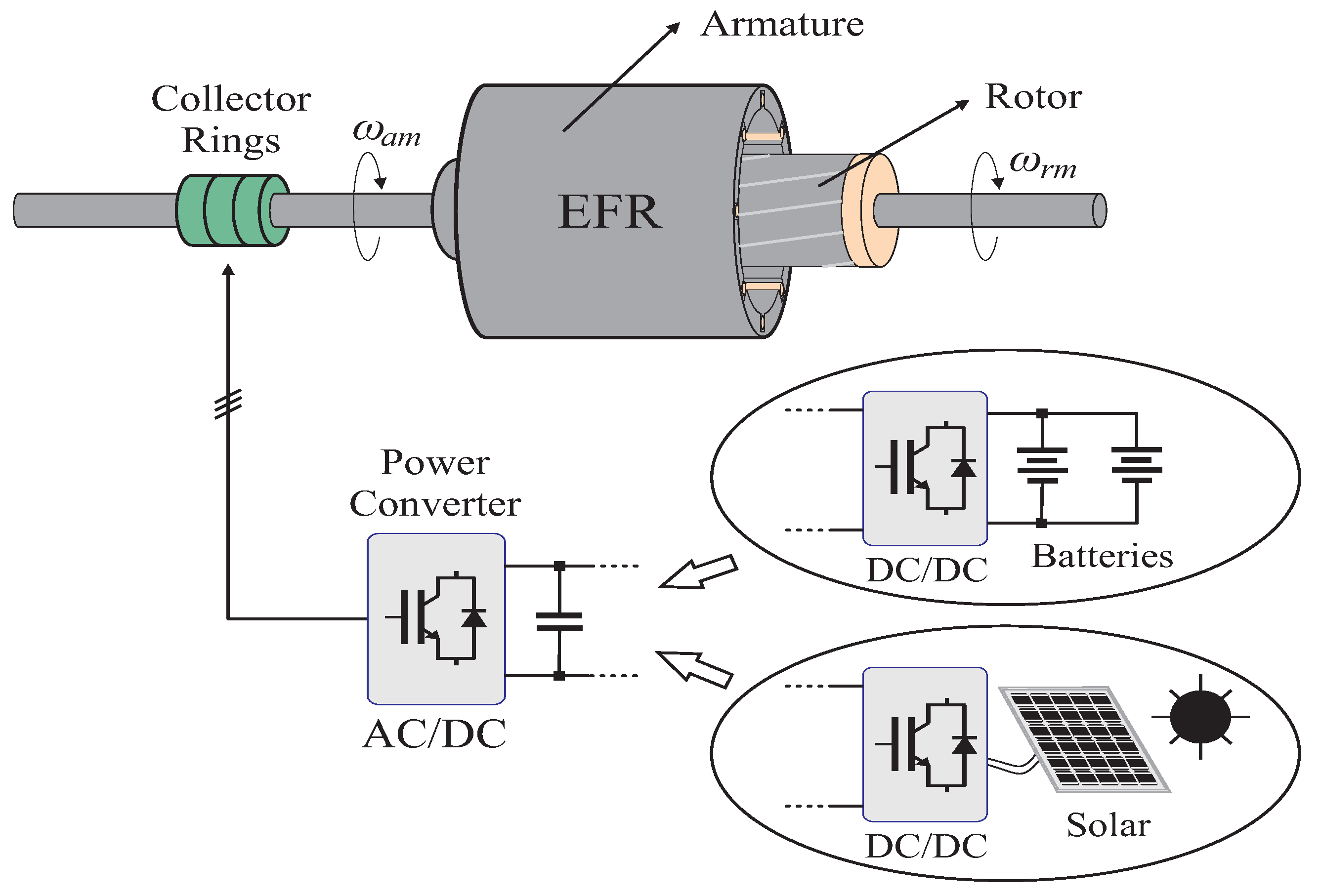
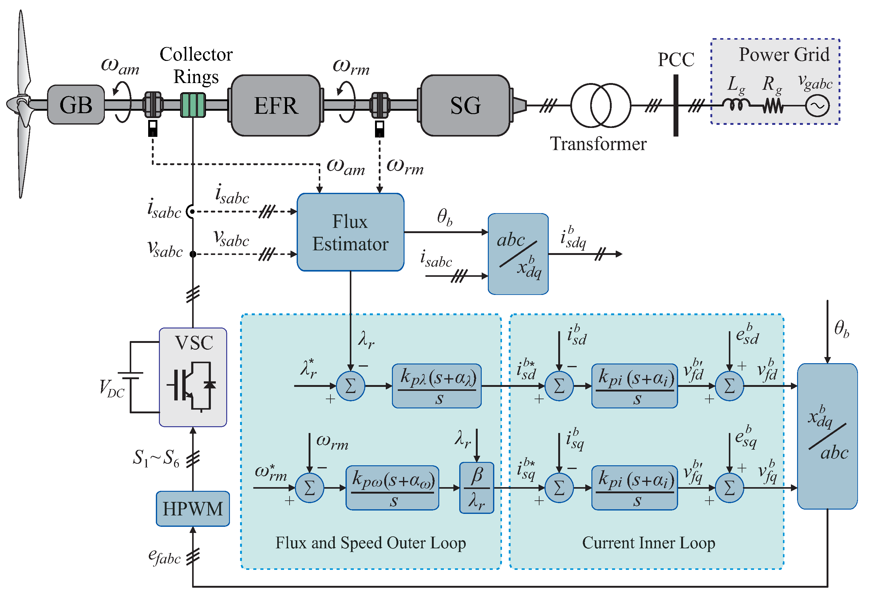
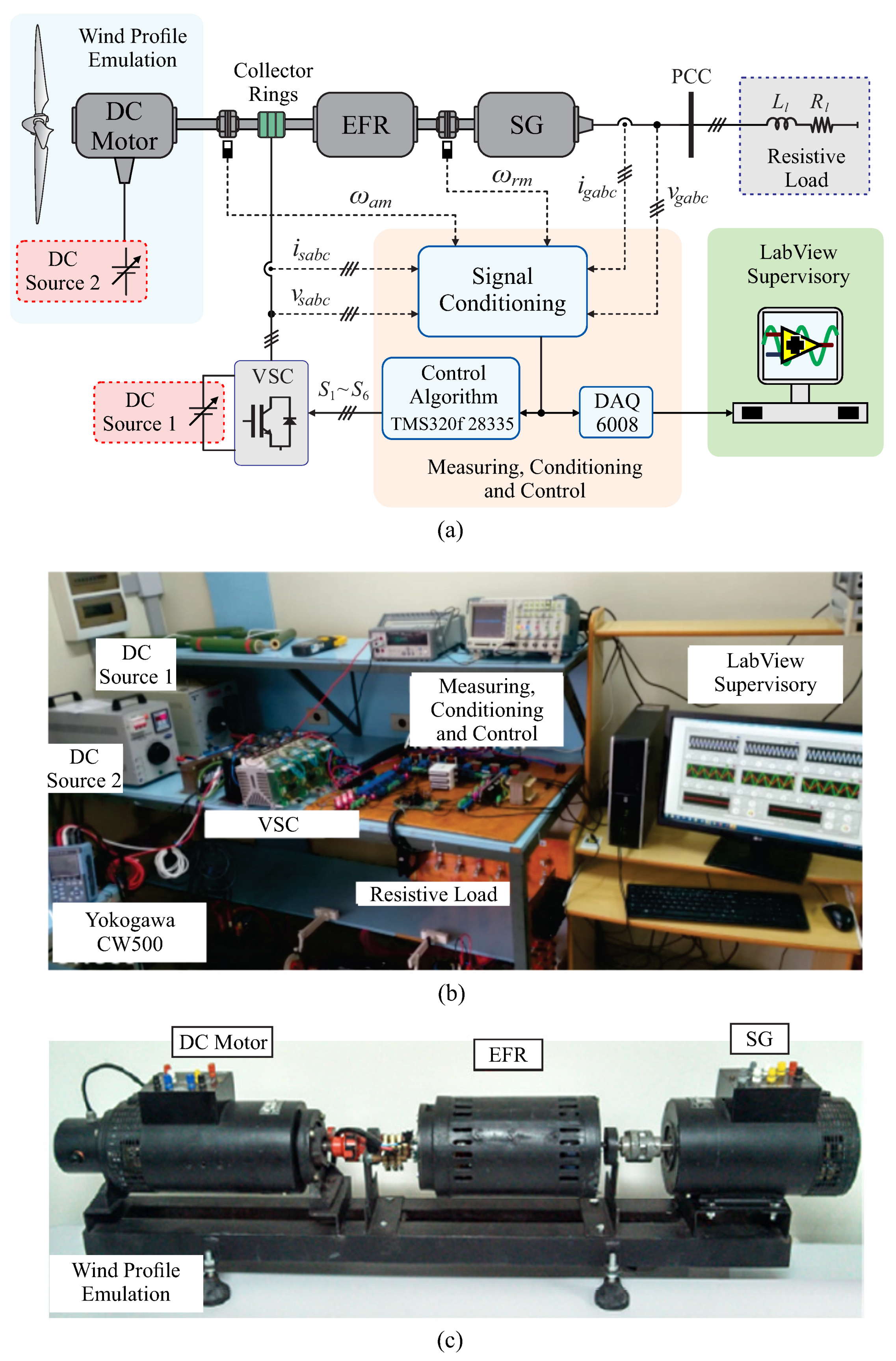
2. System Description and Control Strategy

Figure 2 shows the topology and control scheme of the wind systems employed in this study. A wind turbine is mechanically coupled to the EFR’s armature axis using a gearbox (GB), since its speed is significantly lower than the rotating field speed needed to generate voltage at the grid frequency. A three-phase voltage-source converter (VSC) is employed to regulate the EFR’s armature current and provide a desired angular speed to the synchronous generator (SG) rotor despite the variable angular speed of the wind turbine. Due to the rotational motion of the EFR’s armature axis, collector rings are employed to connect the VSC to the armature windings terminals. The primary source of the EFR-connected converter (i.e., photovoltaic system with energy storage) is emulated by a DC voltage source. The SG stator windings are connected to the point of common coupling (PCC) through a three-phase transformer to adjust the generated voltage values to the power grid voltages. An ideal three-phase voltage source represents the power grid interconnected to the PCC through an equivalent grid impedance composed of series-connected inductor $L_g$ and resistor $R_g$.

Figure 2. Topology of the wind system with EFR and its control strategy.

As shown in Figure 2, the rotor flux field orientation control strategy implemented in this work consists of an outer control loop that regulates the EFR’s rotor flux and speed in cascade with an inner control loop to the EFR’s armature currents. In this control strategy, the system’s dynamic performance is assessed by tuning standard PI controllers. The orthogonal transformations from the $abc$ natural reference frame to the $dq$ field-oriented reference frame employ the phase-angle ${\theta }_b$ provided by a flux estimator, which also determines the EFR rotor flux instantaneous value for feedback in the flux loop. In this work, the reference value ${\omega }_{rm}^{*}$ can be determined according to the maximum power-point tracking (MPPT) operation of the wind turbine as discussed in [14]. The flux controller output determines the reference value $i_{sd}^{*}$ for d-axis armature current control, while the reference value $i_{sq}^{*}$ used in q-axis armature current control is adjusted by the speed controller output. The reference voltages $e_{fabc}$ determined by the inner loop is applied via the hybrid pulse width modulation (HPWM) technique [17], which determines the drive signals of power converter $S_1\sim S_6$.

3. EFR Slip and Dynamic Modeling

3.1. EFR Slip

As mentioned earlier, the EFR device consists of an induction machine with a squirrel-cage rotor and a rotating armature. In this case, the armature windings current produces a rotating field with an absolute angular speed ${\omega }_{sm}$ in mechanical radians per second given by:

$${\omega }_{sm}={\omega }_{am}+\frac{2}{P_{efr}}{\omega }_i,$$

(1)

where ${\omega }_{am}$ and ${\omega }_i$ represent the EFR’s armature angular speed imposed by the wind turbine and the angular frequency of the current in the EFR’s armature windings, respectively. The $P_{efr}$ term represents the EFR poles number. Thus, when the rotor is rotating with a constant speed ${\omega }_{rm}$ in mechanical radians per second, the relative speed per unit or slip between the rotor and the armature rotating field is defined as:

$$s_{efr}=\frac{{\omega }_{sm}-{\omega }_{rm}}{{\omega }_{sm}}=\frac{{\omega }_{am}+\frac{2}{P_{efr}}{\omega }_i-{\omega }_{rm}}{{\omega }_{am}+\frac{2}{P_{efr}}{\omega }_i}.$$

(2)

On the other hand, the induced voltages in the rotor windings due to the armature rotating field have an angular frequency equal to the slip speed in mechanical radians per second given by:

$$s_{efr}{\omega }_{sm}=s_{efr}\left({\omega }_{am}+\frac{2}{P_{efr}}{\omega }_i\right).$$

(3)

Since the rotor windings are short-circuited, the induced voltages will cause currents to flow in the rotor circuit with an amplitude proportional to the induced voltage amplitude and rotor-windings impedance at the slip frequency. Similar to armature currents, rotor currents will establish their rotating field with speed $s_{efr}{\omega }_{sm}$ relative to the rotor. Since the rotor itself is rotating with speed ${\omega }_{rm}$, the absolute speed of the rotor rotating field is defined as:

$${\omega }_{rm}+s{\omega }_{sm}={\omega }_{rm}+\left(\frac{{\omega }_{sm}-{\omega }_{rm}}{{\omega }_{sm}}\right){\omega }_{sm}={\omega }_{sm}.$$

(4)

According to (4), the rotating fields related to the EFR’s armature and rotor rotate with the same absolute speed, which is similar to conventional induction machines.

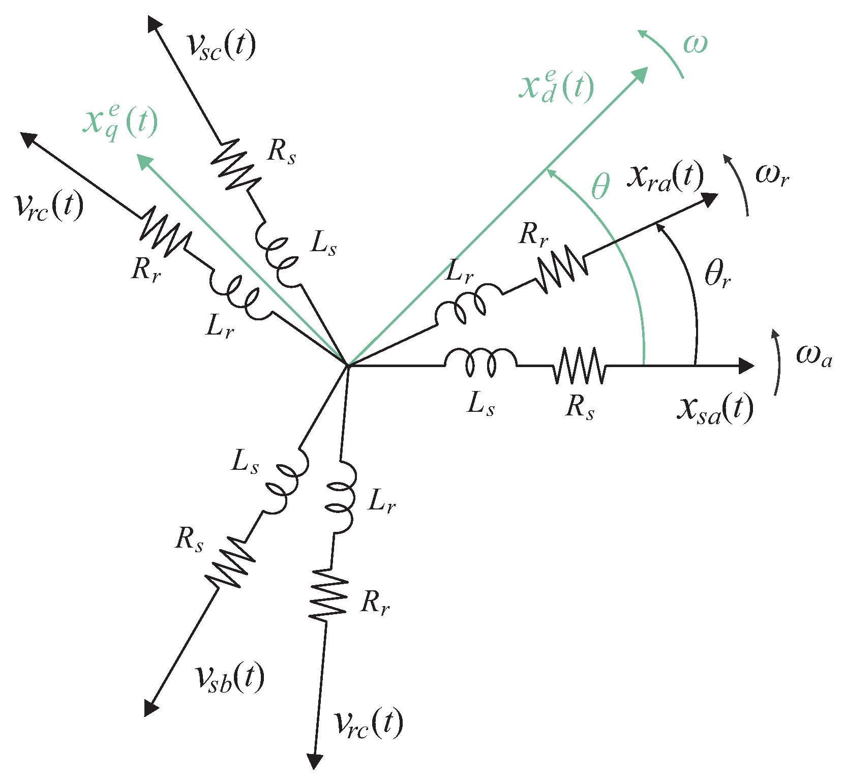
3.2. EFR Dynamic Modeling

Figure 3 shows the armature and rotor $abc$ variables in a natural reference frame and $dq$ variables in an arbitrary reference frame. $L_s$ and $L_r$ represent the self-inductances of the armature and rotor windings, respectively, which also have intrinsic resistances equal to $R_s$ and $R_r$.

Figure 3. Relationship between $abc$ and $dq$ variables.

According to Figure 3, $\theta$ represents the angular difference between the d-axis of the arbitrary reference frame and the a-axis of the armature windings, which is expressed as:

$$\theta ={\int }_0^t\left(\omega -{\omega }_a\right)dt,$$

(5)

where $\omega$ represents the rotation speed of the arbitrary d-axis, while ${\omega }_a$ represents the armature rotating speed in electrical radians per second.

On the other hand, ${\theta }_r$ is the angular difference between the a-axes of the armature and rotor windings, which is given by:

$${\theta }_r={\int }_0^t\left({\omega }_r-{\omega }_a\right)dt,$$

(6)

in which ${\omega }_r$ represents the rotor’s rotational speed in electrical radians per second. The $\theta$ and ${\theta }_r$ angles described in (5) and (6) are used to obtain the armature and rotor $dq$ variables.

Considering the EFR device a symmetrical induction machine, without magnetic saturation and with flux sinusoidal distribution, and then applying Kirchhoff’s voltage law to the three-phase circuit composed by the armature and rotor windings, it is possible to obtain its characteristic equations given by:

$${\overrightarrow{v}}_s^e=R_s{\overrightarrow{i}}_s^e+\frac{d{\overrightarrow{\lambda }}_s^e}{dt}+j\left(\omega -{\omega }_a\right){\overrightarrow{\lambda }}_s^e,$$

(7)

$$0=R_r{\overrightarrow{i}}_s^e+\frac{d{\overrightarrow{\lambda }}_r^e}{dt}+j\left(\omega -{\omega }_r\right){\overrightarrow{\lambda }}_r^e,$$

(8)

in which

$${\overrightarrow{\lambda }}_s^e=\left(L_s-L_{sm}\right){\overrightarrow{i}}_s^e+\frac{3}{2}{L}_{sr}{\overrightarrow{i}}_r^e,$$

(9)

$${\overrightarrow{\lambda }}_r^e=\left(L_r-L_{rm}\right){\overrightarrow{i}}_r^e+\frac{3}{2}{L}_{sr}{\overrightarrow{i}}_s^e,$$

(10)

represent the armature and rotor $dq$ flux linkages, respectively. The superscript e denotes the arbitrary $dq$ reference frame, while any variable $\overrightarrow{x}$ in these equations represents vectors expressed as:

$$\overrightarrow{x}=\frac{1}{\sqrt{2}}\left(x_d+j{x}_q\right).$$

(11)

The $L_{sm}$ and $L_{rm}$ terms represent the mutual inductance between two windings in the armature and the mutual inductance between two windings in the rotor, respectively, while $L_{sr}$ is mutual inductance between the stator and rotor windings. The electromagnetic conjugate of the EFR device can be computed as:

$$T_{em}=\frac{3P{L}_{sr}}{2}\left({\overrightarrow{i}}_r^e\times {\overrightarrow{i}}_s^e\right),$$

(12)

where the × operator represents the vector product between ${\overrightarrow{i}}_r^e$ and ${\overrightarrow{i}}_s^e$ current vectors.

The mechanical motion related to the EFR’s armature can be described by the swing equation given by:

$$T_{am}-T_{em}=J_a\frac{d{\omega }_{am}}{dt}+f_{am}{\omega }_{am},$$

(13)

in which $J_a$ is the total inertia of the wind turbine coupled to the rotating armature on the high-speed side of the gearbox and $f_{am}$ is the armature friction factor. The swing equation for the EFR rotor’s mechanical motion is given by:

$$T_{em}-T_{rm}=J_r\frac{d{\omega }_{rm}}{dt}+f_{rm}{\omega }_{rm},$$

(14)

where $J_r$ is the sum of the inertia of the EFR rotor with the SG rotor, and $f_{rm}$ is the rotor friction factor. The $T_{am}$ term represents the wind turbine mechanical conjugate at the high-speed side of the gearbox, while $T_{rm}$ represents the mechanical conjugate applied to the EFR rotor.

The referential frame for the $dq$ quantities in (7)–(12) is chosen according to the control technique implemented. For the rotor-flux-field-orientation method employed in this work, the arbitrary d-axis is aligned with the rotor-flux-vector axis, which results in decoupling between the flux and conjugate loops [18,19]. Thus, considering the rotor-flux-field-orientation reference frame, it is possible to obtain the transfer functions which will be used in the design and performance analysis of the system controllers.

3.2.1. Armature Current Model

The mathematical model employed to evaluate the dynamic behavior of EFR’s armature current can be obtained from (7)–(10), which results in the equations:

$$v_{sd}^e=R_{sr}{i}_{sd}^e+\sigma \frac{d{i}_{sd}^e}{dt}+e_{sd}^e,$$

(15)

$$v_{sq}^e=R_{sr}{i}_{sq}^e+\sigma \frac{d{i}_{sq}^e}{dt}+e_{sq}^e,$$

(16)

in which

$$e_{sd}^e=-\left(\omega -{\omega }_a\right)\sigma i_{sq}^e-\left({\omega }_r-{\omega }_a\right)\left(\frac{1.5L_{sr}}{L_r-L_{rm}}\right){\lambda }_{rq}^e-\frac{1.5L_{sr}{R}_r}{{\left(L_r-L_{rm}\right)}^2}{\lambda }_{rd}^e.$$

(17)

$$e_{sq}^e\left(t\right)=\left(\omega -{\omega }_a\right)\sigma i_{sd}^e\left(t\right)+\left({\omega }_r-{\omega }_a\right)\left(\frac{1.5L_{sr}}{L_r-L_{rm}}\right){\lambda }_{rd}^e\left(t\right)-\frac{1.5L_{sr}{R}_r}{{\left(L_r-L_{rm}\right)}^2}{\lambda }_{rq}^e\left(t\right),$$

(18)

represents disturbances to be compensated for at the current-controller output as illustrated in Figure 2. The $\sigma$ and $R_{sr}$ terms are constants given by:

$$R_{sr}=R_s+R_r{\left(\frac{1.5L_{sr}}{L_r-L_{rm}}\right)}^2,$$

(19)

$$\sigma =L_s-L_{sm}-\frac{2.25L_{sr}^2}{L_r-L_{rm}}.$$

(20)

Assuming the rotor-flux-field-orientation reference frame defined by ${\lambda }_{rd}^b={\lambda }_r$, ${\lambda }_{rq}^b=0$ and $\omega ={\omega }_b$ [18], (15) and (16) can be rewritten as:

$$v_{sd}^b=R_{sr}{i}_{sd}^b+\sigma \frac{d{i}_{sd}^b}{dt}+e_{sd}^b,$$

(21)

$$v_{sq}^b=R_{sr}{i}_{sq}^b+\sigma \frac{d{i}_{sq}^b}{dt}+e_{sq}^b,$$

(22)

in which

$$e_{sd}^b=-\left({\omega }_b-{\omega }_a\right)\sigma i_{sq}^b-\frac{1.5L_{sr}{R}_r}{{\left(L_r-L_{rm}\right)}^2}{\lambda }_r,$$

(23)

$$e_{sq}^b=\left({\omega }_b-{\omega }_a\right)\sigma i_{sd}^b+\left({\omega }_r-{\omega }_a\right)\left(\frac{1.5L_{sr}}{L_r-L_{rm}}\right){\lambda }_r.$$

(24)

The superscript b denotes the rotor-flux-field-orientation reference frame. Assuming $v_{sd}^{b^{\prime }}=v_{sd}^b-e_{sd}^b$ and $v_{sq}^{b^{\prime }}=v_{sq}^b-e_{sq}^b$, and then applying Laplace transformation in (21) and (22), it is possible to obtain a transfer function defined as:

$$G_i\left(s\right)=\frac{I_{sdq}^b\left(s\right)}{V_{sdq}^{b^{\prime }}\left(s\right)}=\frac{1}{\sigma s+R_{sr}}.$$

(25)

The transfer function given in (25) describes the dynamic relationship between the armature current and voltage in the rotor-flux-field-orientation reference frame.

3.2.2. Rotor Flux Model

Similarly, the model employed to evaluate the dynamic behavior of EFR’s rotor flux can also be obtained from (7)–(10), which results in the expression given by:

$$\frac{1.5L_{sr}}{{\tau }_r}{i}_{sd}^e=\frac{1}{{\tau }_r}{\lambda }_{rd}^e+\frac{d{\lambda }_{rd}^e}{dt}-\left(\omega -{\omega }_r\right){\lambda }_{rq}^e,$$

(26)

in which

$${\tau }_r=\frac{L_r-L_{rm}}{R_r}.$$

(27)

Assuming the rotor-flux-field-orientation reference frame, i.e., ${\lambda }_{rd}^b={\lambda }_r$, ${\lambda }_{rq}^b=0$ and $\omega ={\omega }_b$, (26) can be rewritten as:

$$\frac{1.5L_{sr}}{{\tau }_r}{i}_{sd}^b=\frac{1}{{\tau }_r}{\lambda }_r+\frac{d{\lambda }_r}{dt}.$$

(28)

Applying Laplace transformation in (28), it is possible to obtain the transfer function, defined as:

$$G_{{\lambda }_r}\left(s\right)=\frac{{\Lambda }_r\left(s\right)}{I_{sd}^b\left(s\right)}=\frac{1.5L_{sr}}{{\tau }_{r}s+1},$$

(29)

which correlates the d-axis armature current with the rotor flux.

3.2.3. Rotor Speed Model

From (10) and (12), the electromagnetic conjugate can be expressed as follows:

$$T_{em}=P_{efr}\frac{1.5L_{sr}}{L_r-L_{rm}}\left({\lambda }_{rd}^e{i}_{sq}^e-{\lambda }_{rq}^e{i}_{sd}^e\right),$$

(30)

in which adopting the rotor-flux-field-orientation reference frame results in the following expression:

$$\begin{array}{c}{T}_{em}=P_{efr}\frac{1.5L_{sr}}{L_r-L_{rm}}{\lambda }_r{i}_{sq}^b=\frac{1}{\beta }{\lambda }_r{i}_{sq}^b,\hfill \end{array}$$

(31)

in which

$$\beta =\frac{\left(L_r-L_{rm}\right)}{1.5P_{efr}{L}_{sr}}.$$

(32)

Since the d-axis armature current is directly related to the rotor flux and the q-axis armature current is directly related to the electromagnetic conjugate as expressed in (28) and (31), respectively, it is possible to obtain decoupling between the flux and conjugate control loops of the EFR device.

From (14), it is possible to obtain a dynamic relationship between the electromagnetic conjugate and the rotor speed. Thus, substituting (31) in (14), and assuming the mechanical conjugate $T_{rm}$ as a disturbance to the control action, results in the following expression:

$$\frac{{\lambda }_r}{\beta }{i}_{sq}^b=J_r\frac{d{\omega }_{rm}}{dt}+f_{rm}{\omega }_{rm}.$$

(33)

Considering rotor flux magnitude constant, i.e., ${\lambda }_r\approx {\lambda }_{rn}$, and then applying the Laplace transformation in (33), it is possible obtain the following transfer function:

$$G_{{\omega }_r}\left(s\right)=\frac{{\Omega }_{rm}\left(s\right)}{I_{sq}^b\left(s\right)}=\frac{{\lambda }_{rn}}{\beta \left(J_{r}s+f_{rm}\right)},$$

(34)

in which ${\lambda }_{rn}$ represents the EFR’s rated rotor flux.

The model given in (34) describes the dynamic relationship between rotor speed and q-axis armature current, which in turn is directly related to the electromagnetic conjugate.

4. EFR’s Dynamic Analysis

The dynamic analysis implements the current, flux and speed models obtained in the previous section in order to obtain the dynamic behavior of the EFR device under parametric variations. This analysis employs the parameters listed in Table 1.

Table 1. EFR’s parameters.

	Parameter	Value
EFR device	Poles number ($P_{efr}$)	2
	Armature inductance ($L_s$)	242 mH
	Rotor inductance ($L_r$)	242 mH
	Armature resistance ($R_s$)	$5.795 \Omega$
	Rotor resistance ($R_r$)	$5.795 \Omega$
	Armature mutual inductance ($L_{sm}$)	121 mH
	Rotor mutual inductance ($L_{rm}$)	121 mH
	Armature-to-rotor inductance ($L_{sr}$)	265 mH
	Rotor inertia moment ($J_r$)	$0.02$ kg·m2
	Rotor friction factor ($f_{rm}$)	$0.003$ N·m/rad·s−1

4.1. Transient Response Analysis

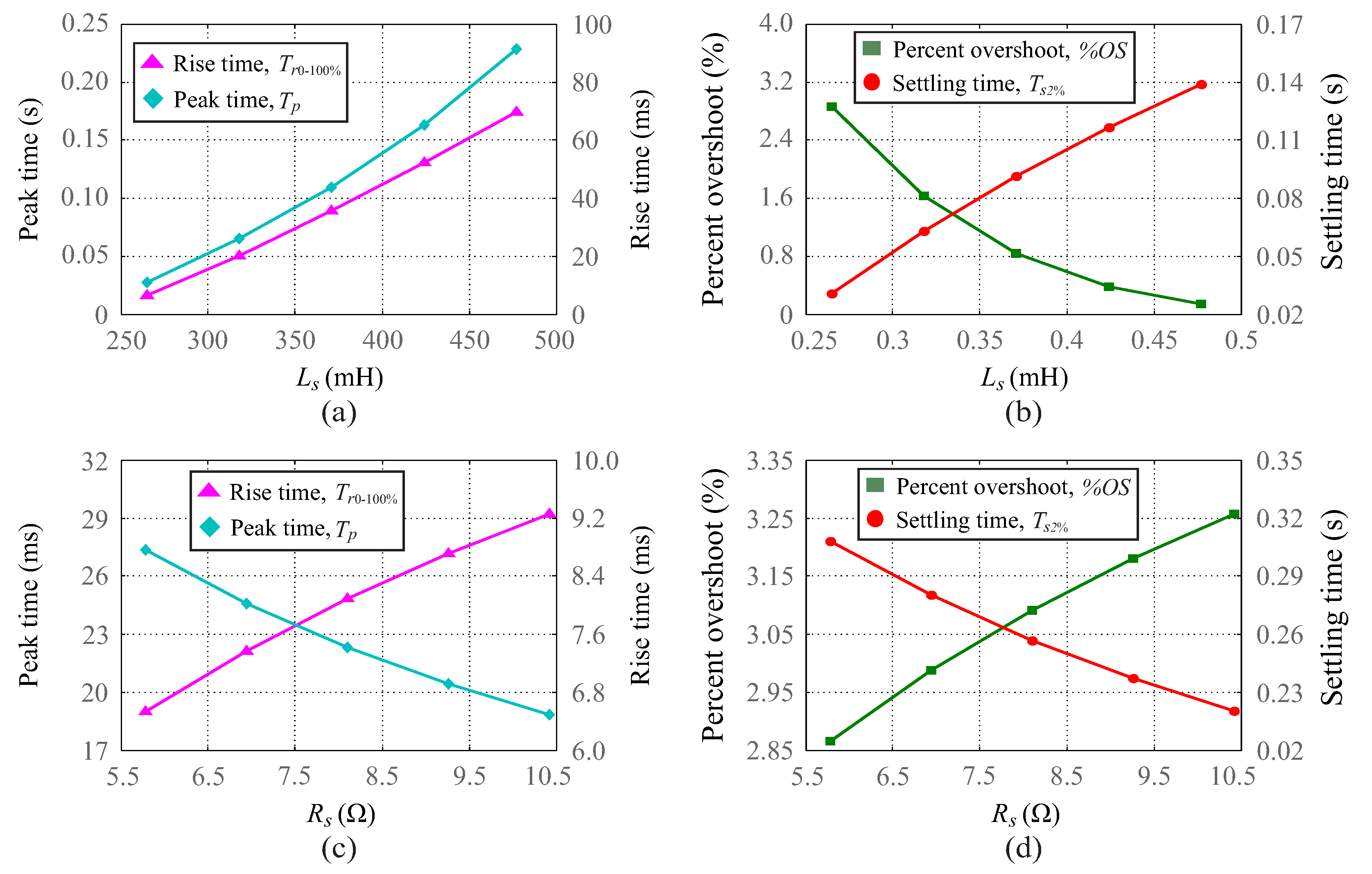
4.1.1. Current Transient Response

Since the transfer function given in (25) is a first-order system, the armature current transient response can be evaluated by specifying settling time ($T_{s2\%}$), defined as [20]:

$$T_{s2\%}=\frac{4}{a}=\frac{4\sigma }{R_{sr}},$$

(35)

where $a=R_{sr}/\sigma$ represents the open-loop system pole. According to (35), the settling time value depends on the armature and rotor windings impedance of the EFR.

Figure 4 shows the settling time assuming variations in the inductance and resistance of the EFR armature. In this case, armature inductance and resistance were increased with an increment rate of 20% around their values defined in Table 1. According to Figure 4a, when $L_s$ armature inductance increases from 260 to 480 mH, the settling time increases from 15 to 95 ms, approximately, which represents a degradation to armature current transient performance. On the other hand, according to Figure 4b, when $R_s$ armature resistance increases from $5.6$ to $10.4 \Omega$, the settling time decreases from 140 to 35 ms, approximately, which may represent an improvement on the transient performance. Therefore, armature current transient behavior is influenced by EFR’s parameters.

Figure 4. Settling time for variations in the (a) $L_s$ armature inductance (b) $R_s$ armature resistance.

4.1.2. Flux Transient Response

According to the rotor flux field orientation method, the rotor flux loop is nested to the d-axis armature current loop. Thus, from (25) and (29), it is possible to obtain a direct relationship between rotor flux and d-axis armature voltage expressed by the following transfer functions:

$$G_{\lambda i}\left(s\right)=G_{{\lambda }_r}\left(s\right)G_i\left(s\right)=\frac{{\Lambda }_r\left(s\right)}{V_{sd}^{b^{\prime }}\left(s\right)}=\frac{\frac{1.5L_{sr}}{{\tau }_r\sigma }}{s^2+\left(\frac{{\tau }_r{R}_{sr}+\sigma }{{\tau }_r\sigma }\right)s+\frac{R_{sr}}{{\tau }_r\sigma }}.$$

(36)

The model described by (36) represents a second-order system in which pole locations vary as a function of the armature and rotor impedance parameters of the EFR. Thus, by matching the dynamic model $G_{\lambda i}\left(s\right)$ to the typical second-order transfer function, natural frequency (${\omega }_{\lambda i}$) and the damping ratio (${\xi }_{\lambda i}$) related to this model can be calculated as follows:

$${\omega }_{\lambda i}=\sqrt{\frac{R_{sr}}{{\tau }_r\sigma }},$$

(37)

$${\xi }_{\lambda i}=\frac{{\tau }_r{R}_{sr}+\sigma }{2\sqrt{{\tau }_r\sigma R_{sr}}}.$$

(38)

In this case, the system parameters’ influence on EFR rotor flux transient response can be evaluated by specifications defined as rise time ($T_{r0-100\%}$), peak time ($T_p$), percent overshoot (%$OS$) and settling time ($T_{s2\%}$). Their values are computed by the following expressions [20]:

$$\begin{array}{cc}{T}_{r0-100\%}\hfill & =\frac{\pi -co{s}^{-1}\left({\xi }_{\lambda i}\right)}{{\omega }_{\lambda i}\sqrt{1-{\xi }_{\lambda i}^2}}\hfill \\ & =2{\tau }_r\sigma \left[\frac{\pi -co{s}^{-1}\left(\frac{{\tau }_r{R}_{sr}+\sigma }{2\sqrt{{\tau }_r\sigma R_{sr}}}\right)}{\sqrt{\left(\sigma -{\tau }_r{R}_{sr}\right)\left({\tau }_r{R}_{sr}-\sigma \right)}}\right],\hfill \end{array}$$

(39)

$$T_p=\frac{\pi }{{\omega }_{\lambda i}\sqrt{1-{\xi }_{\lambda i}^2}}=\frac{2\pi {\tau }_r\sigma }{\sqrt{\left(\sigma -{\tau }_r{R}_{sr}\right)\left({\tau }_r{R}_{sr}-\sigma \right)}},$$

(40)

$$\begin{array}{cc}\%OS\hfill & =e^{-\left({\xi }_{\lambda i}\pi /\sqrt{1-{\xi }_{\lambda i}^2}\right)}\times 100\hfill \\ & =e^{-\left[\frac{\left({\tau }_r{R}_{sr}+\sigma \right)\pi }{\sqrt{\left(\sigma -{\tau }_r{R}_{sr}\right)\left({\tau }_r{R}_{sr}-\sigma \right)}}\right]}\times 100,\hfill \end{array}$$

(41)

$$T_{s2\%}=\frac{4}{{\xi }_{\lambda i}{\omega }_{\lambda i}}=\frac{8{\tau }_r\sigma }{{\tau }_r{R}_{sr}+\sigma }.$$

(42)

According to (39)–(42), similar to the case of the current model, the transient response specification values for the flux model also depend on the impedance of the EFR windings. Figure 5 shows the rise time, peak time, percent overshoot and settling time for different armature inductance and resistance values of the EFR. According to Figure 5a,b, when $L_s$ armature inductance increases from 260 to 480 mH, the rise time, peak time and settling time increase, approximately, from 10 to 90 ms, from $0.025$ to $0.225$ s and from $0.03$ to $0.14$ s, respectively, which can represent a degradation in transient performance. On the other hand, percent overshoot decreases from 3% to $0.2$%, approximately, which may represent an improvement in rotor flux transient performance. According to Figure 5c,d, when $R_s$ armature resistance increases from $5.6$ to $10.4 \Omega$, the peak time and settling time decrease, approximately, from 27 to 18 ms and from $0.31$ to $0.22$ s, respectively, which may represent an improvement in rotor flux transient performance. On the other hand, the percent overshoot and rise time increase from $2.9$% to $3.25$% and from $6.5$ to $9.2$ ms, respectively, which can represent a degradation in transient performance. Therefore, rotor flux transient behavior can be greatly influenced by EFR parameters.

Figure 5. Flux transient response specifications for armature winding parameter variations. (a) Rise time and peak time for $L_s$ variations. (b) Percent overshoot and settling time for $L_s$ variations. (c) Rise time and peak time for $R_s$ variations (d) Percent overshoot and settling time for $R_s$ variations.

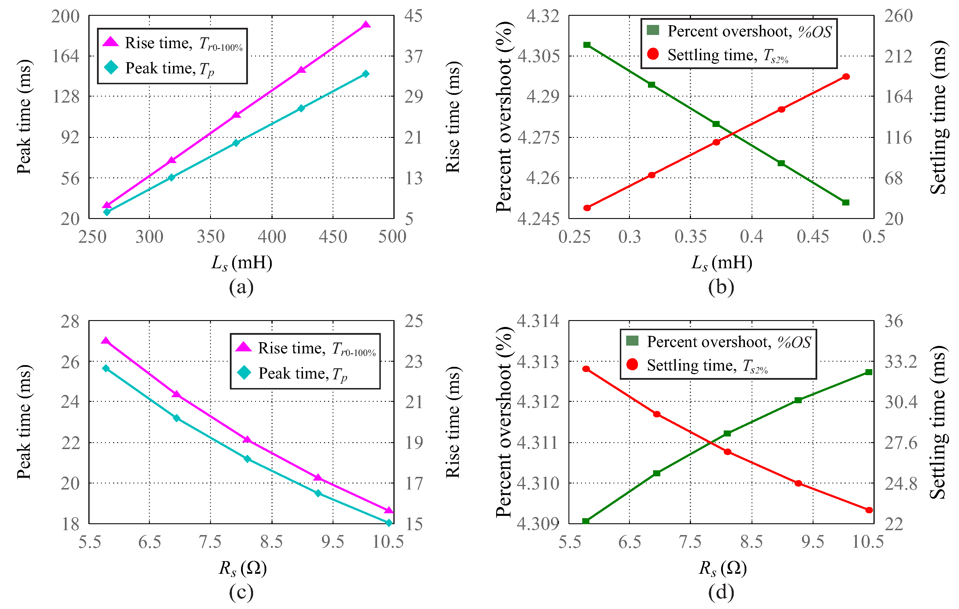
4.1.3. Speed Transient Response

By using a similar procedure, since the rotor speed loop is nested to the q-axis armature current loop, from (25) and (34) it is possible to obtain a transfer function that describes the direct relationship between rotor speed and q-axis armature voltage given by:

$$G_{\omega i}\left(s\right)=G_{{\omega }_r}\left(s\right)G_i\left(s\right)=\frac{{\Omega }_r\left(s\right)}{V_{sq}^{b^{\prime }}\left(s\right)}=\frac{\frac{{\lambda }_{rn}}{J_r\sigma \beta }}{s^2+\left(\frac{J_r{R}_{sr}+f_{rm}\sigma }{J_r\sigma }\right)s+\frac{f_{rm}{R}_{sr}}{J_r\sigma }},$$

(43)

which results in a natural frequency (${\omega }_{\omega i}$) and damping ratio (${\xi }_{\omega i}$) related to this model given by:

$${\omega }_{\omega i}=\sqrt{\frac{f_{rm}{R}_{sr}}{J_r\sigma }},$$

(44)

$${\xi }_{\omega i}=\frac{J_r{R}_{sr}+f_{rm}\sigma }{2\sqrt{J_r\sigma f_{rm}{R}_{sr}}}.$$

(45)

In this case, the transient response specifications of the EFR’s rotor speed can be computed as follows:

$$\begin{array}{cc}{T}_{r0-100\%}\hfill & =\frac{\pi -co{s}^{-1}\left({\xi }_{\omega i}\right)}{{\omega }_{\omega i}\sqrt{1-{\xi }_{\omega i}^2}}\hfill \\ & =2J_r\sigma \left[\frac{\pi -co{s}^{-1}\left(\frac{J_r{R}_{sr}+f_{rm}\sigma }{2\sqrt{J_r\sigma f_{rm}{R}_{sr}}}\right)}{\sqrt{\left(f_{rm}\sigma -J_r{R}_{sr}\right)\left(J_r{R}_{sr}-f_{rm}\sigma \right)}}\right],\hfill \end{array}$$

(46)

$$T_p=\frac{\pi }{{\omega }_{\omega i}\sqrt{1-{\xi }_{\omega i}^2}}=\frac{2\pi J_r\sigma }{\sqrt{\left(f_{rm}\sigma -J_r{R}_{sr}\right)\left(J_r{R}_{sr}-f_{rm}\sigma \right)}},$$

(47)

$$\begin{array}{cc}\%OS\hfill & =e^{-\left({\xi }_{\omega i}\pi /\sqrt{1-{\xi }_{\omega i}^2}\right)}\times 100\hfill \\ & =e^{-\left[\frac{\left(J_r{R}_{sr}+f_{rm}\sigma \right)\pi }{\sqrt{\left(f_{rm}\sigma -J_r{R}_{sr}\right)\left(J_r{R}_{sr}-f_{rm}\sigma \right)}}\right]}\times 100,\hfill \end{array}$$

(48)

$$T_{s2\%}=\frac{4}{{\xi }_{\omega i}{\omega }_{\omega i}}=\frac{8J_r\sigma }{J_r{R}_{sr}+f_{rm}\sigma }.$$

(49)

According to (46)–(49), the transient response specifications for the rotor speed depend on the EFR windings impedance parameters as well as on its parameters of inertia moments and friction factors. Figure 6 shows the behavior of these specifications assuming variations in the inductance and resistance values of the EFR armature. According to Figure 6a,b, when $L_s$ increases from 260 to 480 mH, the rise time, peak time and settling time increase, approximately, from 8 to 44 ms, from 25 to 145 ms and from 30 to 195 ms, respectively, while the percent overshoot decreases from $4.31$% to $4.25$%, approximately. On the other hand, according to Figure 6c,d, when $R_s$ increases from $5.6$ to $10.4 \Omega$, the rise time, peak time and settling time decrease from 24 to 16 ms, from 26 to 18 ms and from 33 to 23 ms, respectively, while the percent overshoot increases from $4.309$% to $4.313$%, approximately. Therefore, lower values for the $L_s/R_s$ ratio result in higher percent overshoot; however, their values were little affected by variations in the armature parameters. On the other hand, the values of the other transient specifications can be greatly influenced by these parameters.

Figure 6. Speed transient response specifications for armature winding parameter variations. (a) Rise time and peak time for $L_s$ variations. (b) Percent overshoot and settling time for $L_s$ variations. (c) Rise time and peak time for $R_s$ variations. (d) Percent overshoot and settling time for $R_s$ variations.

4.2. Steady-State Response Analysis

The steady-state response analysis for models describing the EFR device can be performed by evaluating error specifications for unity feedback systems. For a stable closed-loop system, these specifications can be obtained by the final value theorem [20].

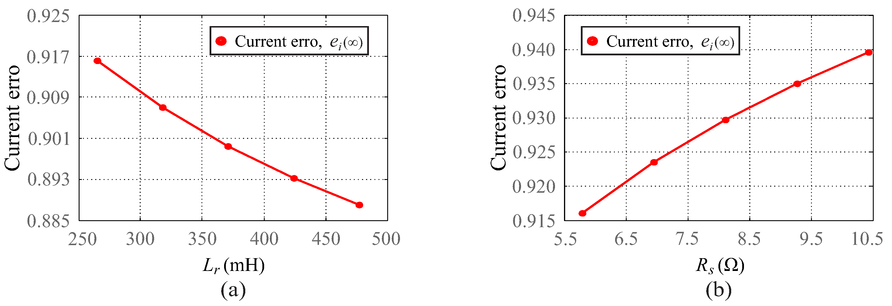
4.2.1. Current Steady-State Response

Considering the model described in (25) and assuming a step input, the steady-state error values for armature current can be defined as:

$$e_i(\infty )=\frac{1}{{\displaystyle 1+\underset{s\to 0}{lim}{G}_i\left(s\right)}}=\frac{R_{sr}}{R_{sr}+1},$$

(50)

where the ${\displaystyle \underset{s\to 0}{lim}{G}_i\left(s\right)}$ term represents static gains computed as:

$${\displaystyle \underset{s\to 0}{lim}{G}_i\left(s\right)=\frac{1}{R_{sr}}.}$$

(51)

According to (50), the steady-state error value of current does not depend on the armature inductance, since it depends only on the parameter $R_{sr}$ described in (19). Figure 7 shows the current steady-state error values for different $L_r$ and $R_s$ parameter values. According to Figure 7a, the error value decreases from $0.916$ to $0.888$ approximately, when $L_r$ increases from 260 to 480 mH. On the other hand, for variations to $R_s$ between $5.6$ to $10.4 \Omega$, the error value increases from $0.916$ to $0.94$, as shown in Figure 7b. Therefore, variations in rotor inductance and armature resistance can modify the armature current steady-state response.

Figure 7. Armature current error values for (a) $L_r$ variations and (b) $R_s$ variations.

4.2.2. Flux and Speed Steady-State Response

The flux and speed steady-state response can be evaluated using the models described in (29) and (34). Thus, assuming these systems have unitary feedback and step inputs, their steady-state error values are defined as:

$$e_{\lambda i}(\infty )=\frac{1}{{\displaystyle 1+\underset{s\to 0}{lim}{G}_{\lambda i}\left(s\right)}}=\frac{R_{sr}}{R_{sr}+1.5L_{sr}},$$

(52)

$$e_{\omega i}(\infty )=\frac{1}{{\displaystyle 1+\underset{s\to 0}{lim}{G}_{\omega i}\left(s\right)}}=\frac{f_{rm}{R}_{sr}\beta }{f_{rm}{R}_{sr}\beta +{\lambda }_{rn}},$$

(53)

in which

$$\begin{array}{c}{\displaystyle \underset{s\to 0}{lim}{G}_{\lambda i}\left(s\right)=\frac{1.5L_{sr}}{R_{sr}},}\hfill \end{array}$$

(54)

$$\begin{array}{c}{\displaystyle \underset{s\to 0}{lim}{G}_{\omega i}\left(s\right)=\frac{{\lambda }_{rn}}{f_{rm}{R}_{sr}\beta }.}\hfill \end{array}$$

(55)

Figure 8 shows the flux and speed steady-state error values for variations of $L_r$ and $R_s$. According to Figure 8a, for variations of $L_r$ between 260 to 480 mH, the flux error value decreases from $0.968$ to $0.956$, while the speed error value increases from $0.014$ to $0.016$, approximately. For variations of $R_s$ between $5.6$ to $10.4 \Omega$, the flux and speed error values increase from $0.968$ to $0.977$ and $0.014$ to $0.02$, respectively, as shown in Figure 8b. Therefore, similar to the current error, variations in rotor inductance and armature resistance can also modify the steady-state response of the rotor flux and speed.

Figure 8. Flux and speed error values for (a) $L_r$ variations and (b) $R_s$ variations.

5. EFR Controller Design

In this section, the EFR controllers are designed by using the RLM and the parameters described in Table 1.

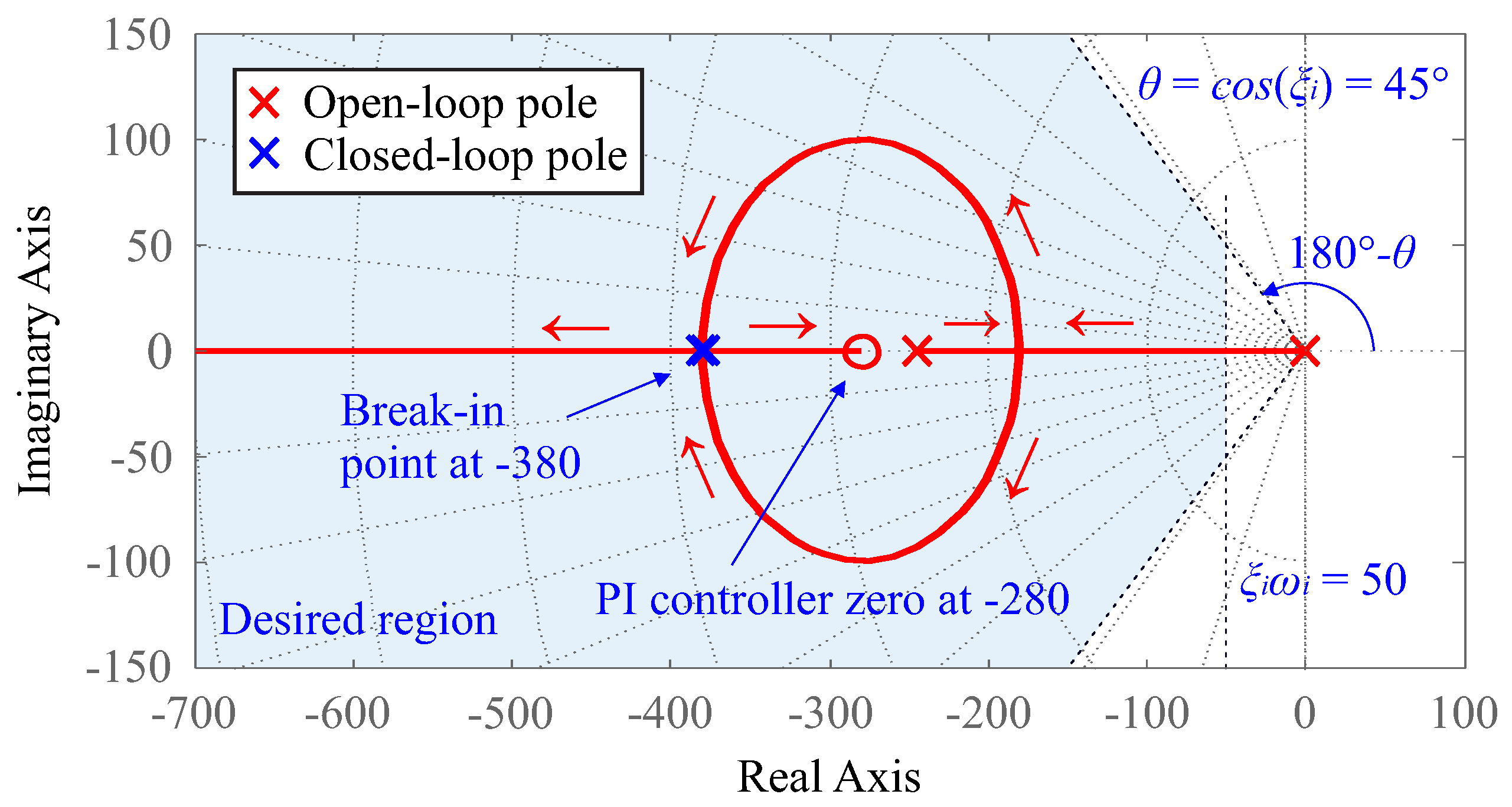
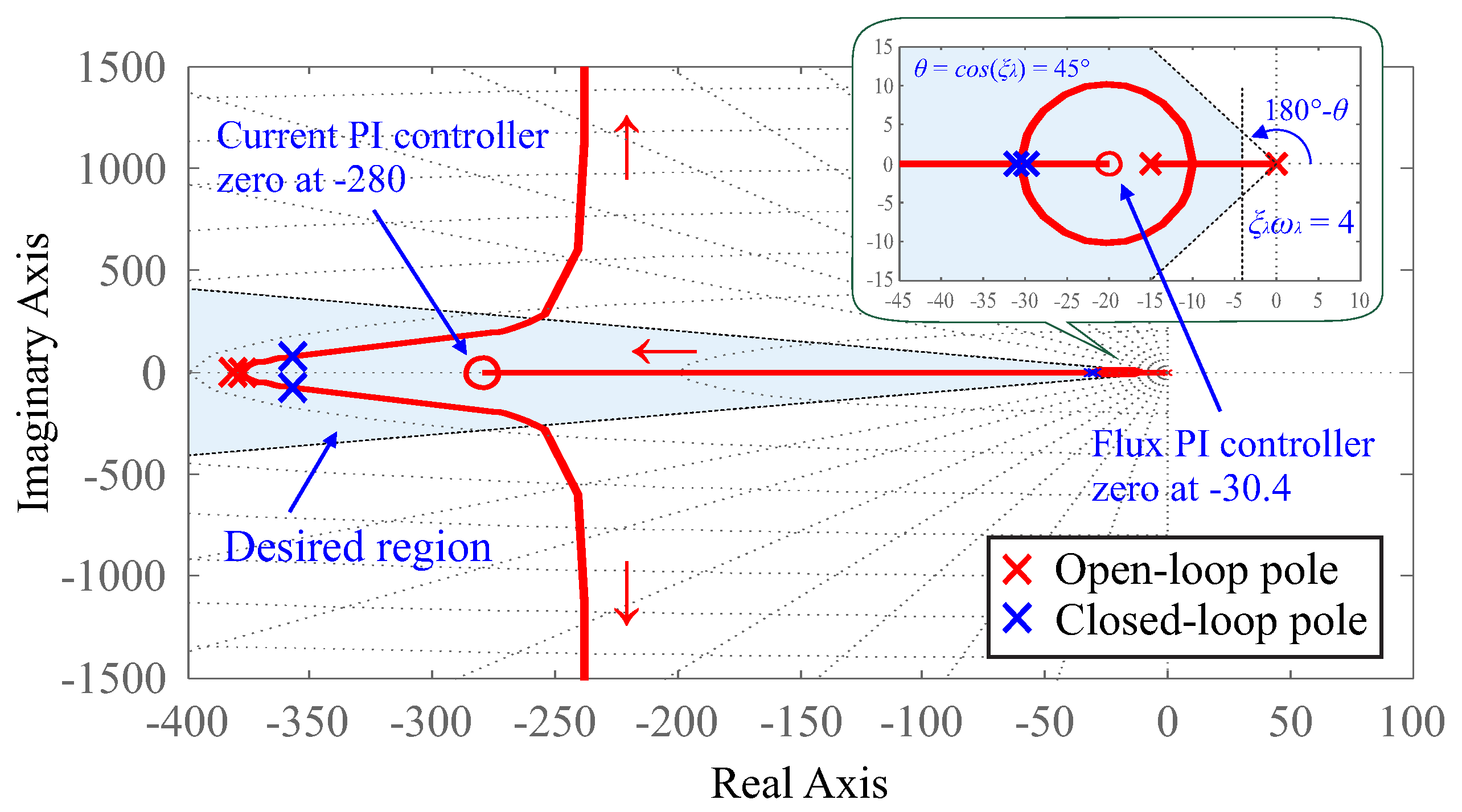
5.1. Current Controller Design

The control strategy employs standard PI controllers for regulating the $dq$ components of the EFR armature current (see Figure 2), whose transfer function given by (25) describes its dynamic behavior. Thus, the EFR current control has an open-loop transfer function described as:

$$H_i\left(s\right)=k_{pi}{T}_i\left(s\right)=\frac{k_{pi}\left(s+{\alpha }_i\right)}{s\left(\sigma s+R_{sr}\right)},$$

(56)

where $k_{pi}$ and ${\alpha }_i$ represent the current PI controller gains.

Since the EFR controllers compose a multi-loop control scheme, the design requirements for the inner control loop are chosen so as not to affect the dynamic performance of the outer control loop [21]. Based on this idea, a percent overshoot (%OS) less than or equal to $5\%$ and a settling time ($T_{s2\%}$) less than or equal to $0.08$ s are used in the design of the current PI controllers. Based on these performance requirements, the minimum value of the natural frequency (${\omega }_i$) and damping ratio (${\xi }_i$) for the closed-loop current control are calculated as follows [20]:

$$\begin{array}{c}{\xi }_i⩾\frac{-ln\left(\%OS/100\right)}{\sqrt{{\pi }^2+l{n}^2\left(\%OS/100\right)}}=\frac{-ln\left(0.05\right)}{\sqrt{{\pi }^2+l{n}^2\left(0.05\right)}}\approx 0.7,\hfill \end{array}$$

(57)

$${\omega }_i⩾\frac{4}{{\xi }_i{T}_{s2\%}}=\frac{4}{0.7\times 0.08}\approx 71.43\mathrm{rad}/\mathrm{s},$$

(58)

and correspond to the desired region for the closed-loop poles illustrated in Figure 9.

Figure 9. Root locus for current control loop.

According to the RLM, the controller zero can be chosen to allow all poles of the closed-loop system to be allocated within the desired region. In this case, this is achieved by setting ${\alpha }_i=280$, which results in the controller zero shown in Figure 9. Then, the $k_{pi}$ gain can be calculated by the module restriction given by the following expression [20]:

$$k_{pi}=\frac{1}{|T_i\left(s_d\right)|}.$$

(59)

The $s_d$ term represents the desired closed-loop pole. In this case, its is allocated in the break-in point on the real axis, which results in $s_d=-380$. Therefore, substituting the value of $s_d$ in (59) results in a controller gain computed as $k_{pi}=22.965$. Figure 9 shows the root locus for the $H_i\left(s\right)$ open-loop system. The closed-loop system has two real and equal poles corresponding to $s_d$, which results in a transient response without percent overshoot.

5.2. Flux Controller Design

The flux control loop is in cascade with the d-axis armature current control loop as shown in Figure 2. Therefore, considering the dynamic model described in (29) and inner current controller dynamics, it is possible to obtain the open-loop transfer function for flux control as follows:

$$\begin{array}{cc}{H}_{\lambda }\left(s\right)\hfill & =k_{p\lambda }{T}_{\lambda }\left(s\right)\hfill \\ & =\frac{1.5L_{sr}{k}_{pi}{k}_{p\lambda }\left(s+{\alpha }_i\right)\left(s+{\alpha }_{\lambda }\right)}{s\left({\tau }_{r}s+1\right)\left(\sigma s^2+\left(R_{sr}+k_{pi}\right)s+k_{pi}{\alpha }_i\right)},\hfill \end{array}$$

(60)

in which $k_{p\lambda }$ and ${\alpha }_{\lambda }$ represent the flux controller gains.

For guaranteeing the proper performance of the multi-loop scheme composed of the flux controller and the d-axis current controller, the design requirements can be chosen so that the control action of the flux outer loop is slower than that of the current inner loop [21]. Thus, assuming $\%OS⩽5$% and $T_{s2\%}⩽1$ s, which results in ${\xi }_{\lambda }⩾0.7$ and ${\omega }_{\lambda }⩾5.714$ rad/s as design criteria, it is possible to obtain the desired region illustrated in Figure 10. In order to allocate all closed-loop poles within this desired region, the zero of the flux PI controller is chosen by setting ${\alpha }_{\lambda }=20$. The $k_{p\lambda }$ gain can be determined by:

$$k_{p\lambda }=\frac{1}{|T_{\lambda }\left(s_d\right)|}.$$

(61)

Figure 10. Root locus for flux control loop.

Therefore, assuming $s_d=-30.4$ results in a control gain computed as $k_{p\lambda }=7.845$. Figure 10 shows the root locus for the $H_{\lambda }\left(s\right)$ open-loop system. The closed-loop system has two real and equal dominant poles that correspond to the $s_d$ adopted and two complex non-dominant poles located furthest from the imaginary axis. In this case, the allocation of non-dominant poles depends on the design requirements adopted for the current inner controller.

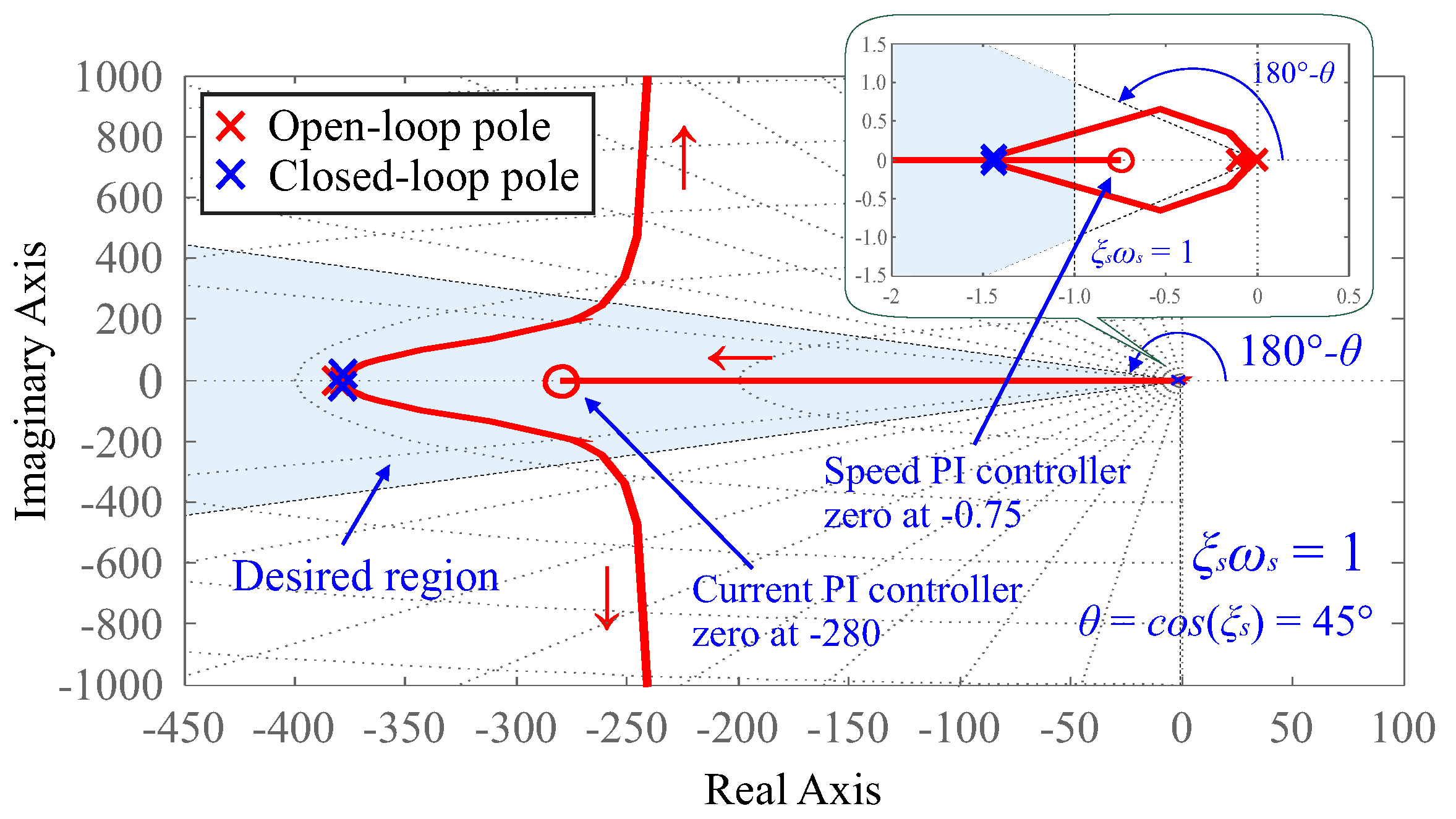
5.3. Speed Controller Design

According to Figure 2, the speed control loop is in cascade with the q-axis armature current control loop. Thus, considering the dynamic model given by (34) and closed-loop current control, it is possible to obtain an open-loop transfer function defined as:

$$\begin{array}{cc}{H}_{\omega }\left(s\right)\hfill & =k_{p\omega }{T}_{\omega }\left(s\right)\hfill \\ & =\frac{k_{p\omega }{k}_{pi}\left(s+{\alpha }_i\right)\left(s+{\alpha }_{\omega }\right)}{s\left(J_{r}s+f_{rm}\right)\left(\sigma s^2+\left(R_{sr}+k_{pi}\right)s+k_{pi}{\alpha }_i\right)},\hfill \end{array}$$

(62)

where $k_{p\omega }$ and ${\alpha }_{\omega }$ represent the speed controller gains.

In this case, the performance requirements applied to the speed controller are $\%OS⩽5$% and $T_{s2\%}⩽4$ s, which results in ${\xi }_s⩾0.7$ and ${\omega }_s⩾1.43$ rad/s. The desired region corresponding to these requirements is shown in Figure 11. Thus, assuming the same procedure employed in the design of flux and current controllers, the speed controller zero is defined by ${\alpha }_{\omega }=0.75$, while the $k_{p\lambda }$ gain can be computed by:

$$k_{p\omega }=\frac{1}{|T_{\omega }\left(s_d\right)|},$$

(63)

in which, assuming $s_d=-1.44$, the controller gain is calculated as $k_{p\omega }=0.0327$. Figure 11 presents the resulting root locus for the speed control loop. According to Figure 11, all closed-loop poles are located within the desired region. In this case, the closed-loop system has two real and equal non-dominant poles that correspond to the closed-loop poles of the current inner loop and are located further from the imaginary axis. In addition, the closed-loop system also has two real and equal dominant poles that are allocated closer to the origin and correspond to the desired pole $s_d$.

Figure 11. Root locus for speed control loop.

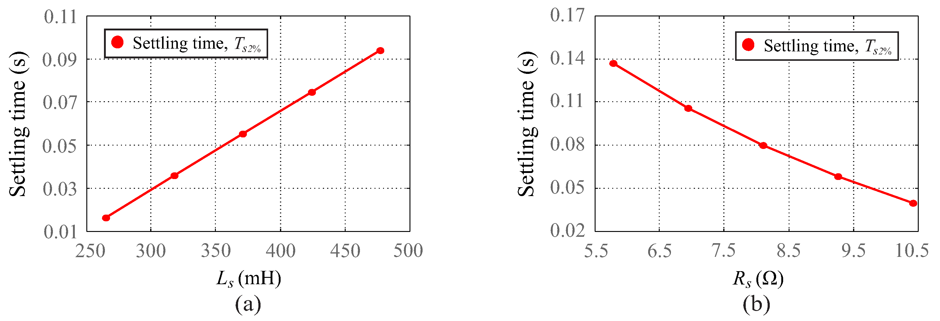
6. Closed-Loop Poles Sensitivity Analysis

In this section, a sensitivity analysis is performed in order to compare the dynamic performance of the system’s controllers assuming variations in the EFR parameters listed in Table 1. This analysis employs the control gains designed in the previous section and summarized in Table 2.

Table 2. Parameter design for system controllers.

	Parameter	Value
Current Controller	Proportional gain ($k_{pi}$)	$22.965$
	Gain (${\alpha }_i$)	280
Flux Controller	Proportional gain ($k_{p\lambda }$)	$7.845$
	Gain (${\alpha }_{\lambda }$)	20
Speed Controller	Proportional gain ($k_{p\omega }$)	$0.0327$
	Gain (${\alpha }_{\omega }$)	$0.75$

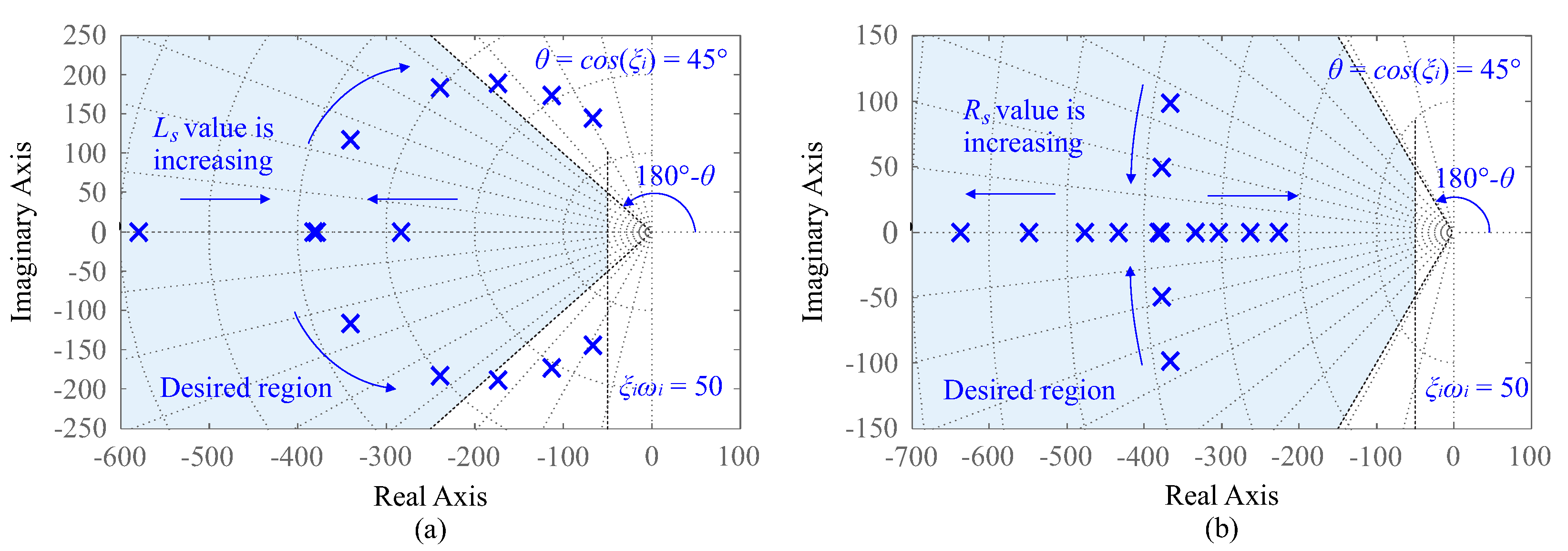
6.1. Current Inner Loop

From the dynamic model given in (56) and assuming systems with unitary feedback, it is possible to obtain the closed-loop transfer function for current control given by:

$$H_{icl}\left(s\right)=\frac{H_i\left(s\right)}{1+H_i\left(s\right)}=\frac{\frac{k_{pi}}{\sigma }\left(s+{\alpha }_i\right)}{s^2+\left(\frac{R_{sr}+k_{pi}}{\sigma }\right)s+\frac{k_{pi}{\alpha }_i}{\sigma }}.$$

(64)

According to (64), the closed-loop current control has two poles whose location depends on the EFR parameters. Figure 12 shows the closed-loop poles’ behavior when $L_s$ and $R_s$ parameters vary. According to Figure 12a, when $L_s$ is increasing, the closed-loop poles are closer to the imaginary axis, which corresponds to a decrease in the system stability margin. In addition, large variations in armature inductance can move the closed-loop poles outside the desired region, which results in degradation of the controller performance. The $R_s$ variation effect in the location of the closed-loop poles is presented in Figure 12b. While $R_s$ is increasing, the complex closed-loop poles are closer to the real axis, which can result in a more dampened transient response. Furthermore, during the variation of $R_s$, the closed-loop poles are allocated within the desired region, which demonstrates the low influence of this parameter on the performance of current controllers.

Figure 12. Closed-loop poles for current control when (a) $L_s$ varies and (b) $R_s$ varies.

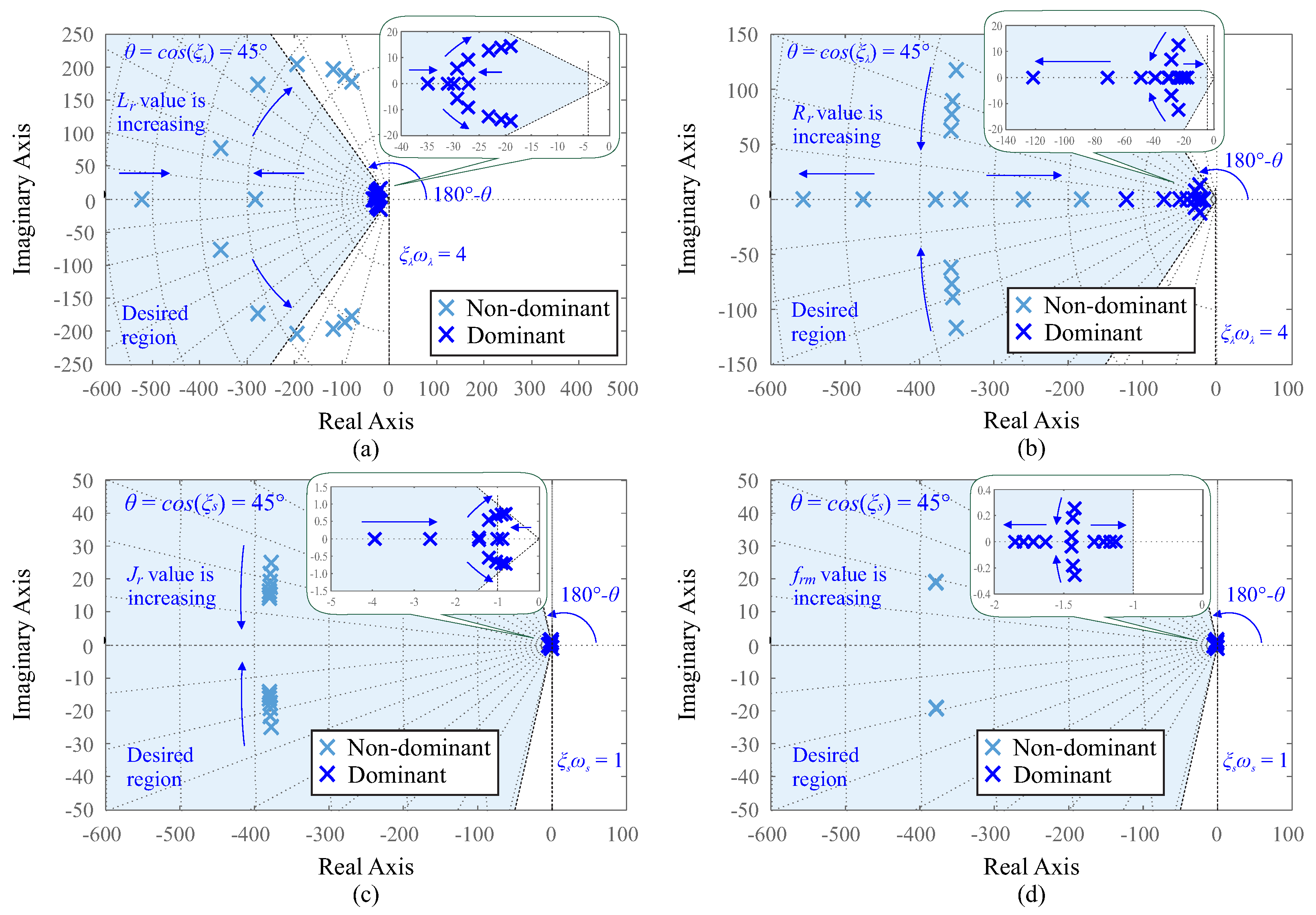
6.2. Flux and Speed Outer Loop

From (60), it is possible to obtain a closed-loop transfer function which describes the flux dynamic behavior, given by:

$$H_{\lambda cl}\left(s\right)=\frac{H_{\lambda }\left(s\right)}{1+H_{\lambda }\left(s\right)}=\frac{\frac{1,5L_{sr}{k}_{pi}{k}_{p\lambda }}{{\tau }_r\sigma }\left(s^2+\left({\alpha }_i+{\alpha }_{\lambda }\right)s+{\alpha }_i{\alpha }_{\lambda }\right)}{s^4+a_3{s}^3+a_2{s}^2+a_{1}s+a_0},$$

(65)

in which

$$a_3=\frac{{\tau }_r\left(R_{sr}+k_{pi}\right)+\sigma }{{\tau }_r\sigma },$$

(66)

$$a_2=\frac{k_{pi}\left(1.5L_{sr}{k}_{p\lambda }+{\tau }_r{\alpha }_i+1\right)+R_{sr}}{{\tau }_r\sigma },$$

(67)

$$a_1=\frac{1.5L_{sr}{k}_{pi}{k}_{p\lambda }\left({\alpha }_i+{\alpha }_{\lambda }\right)+k_{pi}{\alpha }_i}{{\tau }_r\sigma },$$

(68)

$$a_0=\frac{1.5L_{sr}{k}_{pi}{k}_{p\lambda }{\alpha }_i{\alpha }_{\lambda }}{{\tau }_r\sigma }.$$

(69)

According to (65), the closed-loop system has four poles whose localization depends on the EFR parameters. Figure 13a,b shows the effect of $L_r$ and $R_r$ parameter variation in the position of the closed-loop poles for flux control. According to Figure 13a, when $L_r$ is increasing, the non-dominant and dominant poles are closer to the imaginary axis, which corresponds to a decrease in the system stability margin. In addition, large variations in the rotor inductance move the closed-loop poles outside the desired region, which results in degradation of the desired dynamic response. On the other hand, according to Figure 13b, while $R_r$ is increasing, the non-dominant and dominant poles are closer to the real axis, which can result in a less oscillatory transient response. Furthermore, during variation of $R_r$, the closed-loop poles are allocated within the desired region, which demonstrates its low influence on flux controller performance.

Figure 13. Closed-loop poles for (a) flux control when $L_r$ varies, (b) flux control when $R_r$ varies, (c) speed control when $J_r$ varies and (d) speed control when $f_{rm}$ varies.

Similarly, considering the system described in (62), the closed-loop transfer function for speed control is given by:

$$H_{\omega cl}\left(s\right)=\frac{H_{\omega }\left(s\right)}{1+H_{\omega }\left(s\right)}=\frac{\frac{k_{pi}{k}_{p\omega }}{J_r\sigma }\left(s^2+\left({\alpha }_i+{\alpha }_{\omega }\right)s+{\alpha }_i{\alpha }_{\omega }\right)}{s^4+b_3{s}^3+b_2{s}^2+b_{1}s+b_0},$$

(70)

in which

$$b_3=\frac{J_r\left(R_{sr}+k_{pi}\right)+f_{rm}\sigma }{J_r\sigma },$$

(71)

$$b_2=\frac{k_{pi}\left(k_{p\omega }+J_r{\alpha }_i+f_{rm}\right)+f_{rm}{R}_{sr}}{J_r\sigma },$$

(72)

$$b_1=\frac{k_{pi}{k}_{p\omega }\left({\alpha }_i+{\alpha }_{\omega }\right)+f_{rm}{k}_{pi}{\alpha }_i}{J_r\sigma },$$

(73)

$$b_0=\frac{k_{pi}{k}_{p\omega }{\alpha }_i{\alpha }_{\omega }}{J_r\sigma }.$$

(74)

Figure 13c,d show the closed-loop pole behavior of the speed control during variations in $J_r$ and $f_{rm}$. According to Figure 13c, when $J_r$ is increasing, the non-dominant poles are closer to the real axis, while the dominant poles are place outside the desired region and closer to the imaginary axis, which can result in a more oscillatory transient response and a decrease in the system stability margin. On the other hand, according to Figure 13d, when $f_{rm}$ is increasing, the location of the non-dominant poles has negligible change, while the dominant poles are closer to the real axis, which can result in a more dampened transient response. However, the dominant poles are allocated within the desired region, which demonstrates the low influence of $f_{rm}$ parameter variation on the speed controller performance.

7. Simulation and Experimental Results

The EFR-based system parameters for the simulation and experimental study are shown in Table 1, Table 2 and Table 3. The wind turbine parameters used for the simulation and experimental assays were taken from [22]. However, the turbine blade radius and the rated wind speed were adjusted to match the rated turbine and EFR power ratings.

Table 3. EFR-based system’s parameters.

	Parameter	Value
Wind Turbine	Rated power	$1.5$ kW
	Blade radius	2 m
	Rated wind speed	8 m/s
	Air density	$1.225$ kg·m3
	Power coefficient	$0.411$
	Inertia moment ($J_a$)	$0.2$ kg·m2
	Friction factor ($f_{am}$)	$1.0$ N·m/rad·s−1
EFR and SG	Rated power	$1.5$ kW
	SG Poles number	4
	Rated voltage	380 $V_{rms}$
	Rated frequency	$2\pi 60$ rad/s
VSC	DC-Link voltage ($V_{DC}$)	900 V
	Switching frequency ($f_s$)	10 kHz

7.1. Simulation Results

To verify the effectiveness of the proposed performance analysis applied to the EFR-based system, the simulation of the system topology shown in Figure 2 has been carried out using the MATLAB/Simulink software.

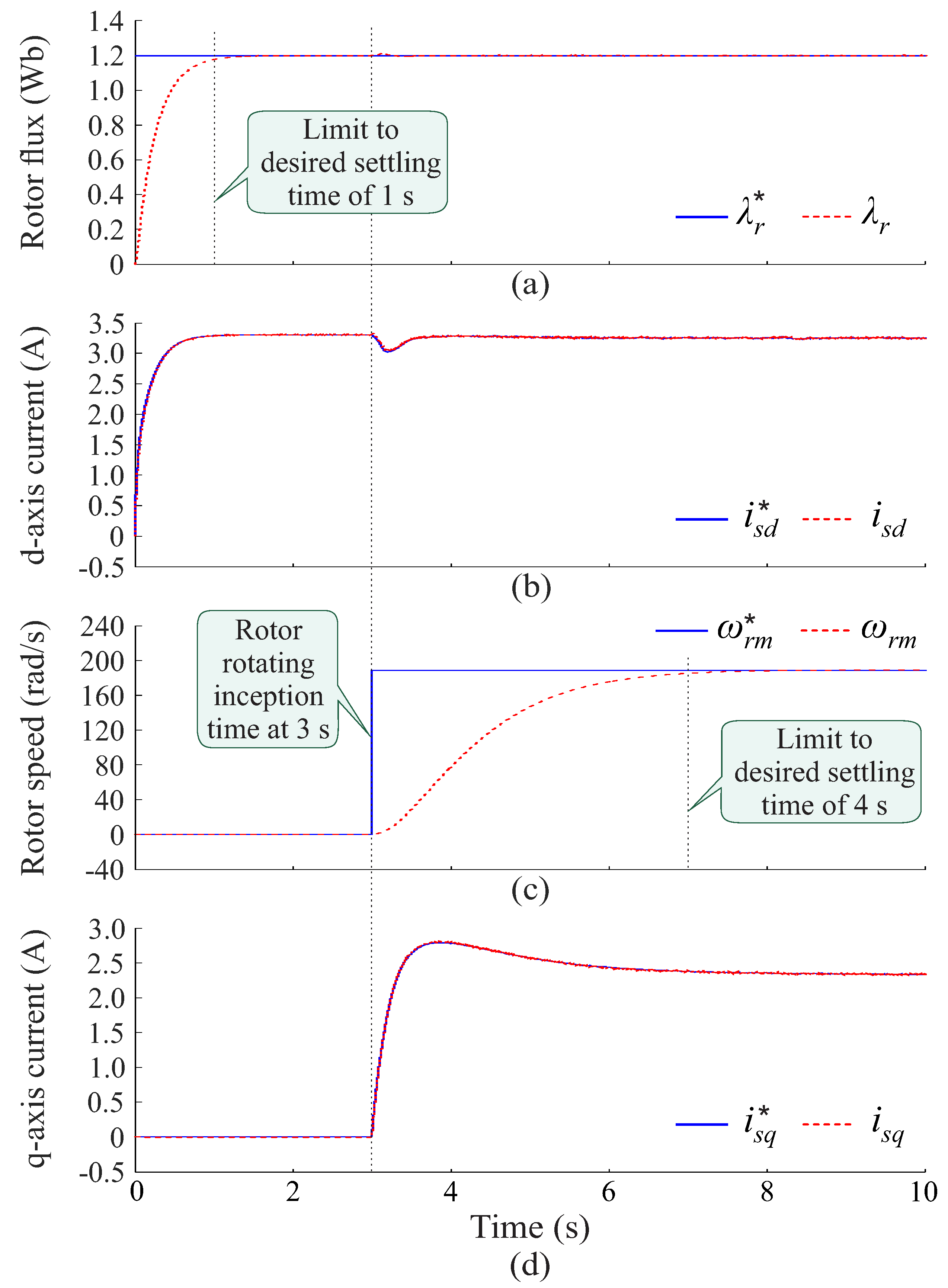
7.1.1. Performance Analysis of the EFR Controllers

Figure 14 shows the dynamic response of the EFR controllers. According to Figure 14a, when the reference signal for the rotor flux changes from 0 to $1.2$ Wb at 0 s, the instantaneous rotor flux tracks this reference value without steady-state error with settling time equal to $0.95$ s, approximately. Then, Figure 14b shows that quickly, in approximately $0.075$ s, the d-axis armature current reaches its reference value. Instantly at $t=3.0$ s, a step from 0 to $188.5$ rad/s is applied to the rotor-speed reference as depicted in Figure 14c. At this speed, as the synchronous generator has 4 poles, the voltage generated presents a frequency of 60 Hz. According to Figure 14c, the rotor speed reaches its reference value accurately in approximately $3.8$ s without percent overshoot. This transition results in the application of an electromagnetic torque to the rotor proportional to the reference value for the q-axis armature current shown in Figure 14d. In this case, similar to the d-axis armature current, the q-axis armature current quickly tracks its reference value. Therefore, in relation to the adopted design criteria, the dynamic performance of the EFR controllers is within the desired limits.

Figure 14. Dynamic responses from system’s controllers (a) rotor flux controller, (b) d-axis armature current controller, (c) rotor speed controller and (d) q-axis armature current controller.

Figure 15 shows the speed controller dynamic response assuming variations in the $J_r$ and $f_{rm}$ parameters around their nominal values listed in Table 1. According to Figure 15a, adopting a 40% lower value for $J_r$, the rise time is reduced, while the settling time and percent overshoot do not change. On the other hand, adopting an 80% higher value for $J_r$, the speed controller transient response presents a higher rise time, settling time and percent overshoot. Then, Figure 15b illustrates the speed controller dynamic performance considering similar variations in $f_{rm}$. In this case, the effect of the variation in $f_{rm}$ was small, since the controller transient responses were almost identical. Therefore, the speed controller dynamic performance assuming variation in $J_r$ and $f_{rm}$ is in accordance with the sensitivity analysis performed in the previous section.

Figure 15. Dynamic response of the speed controller to (a) $J_r$ variations and (b) $f_{rm}$ variations.

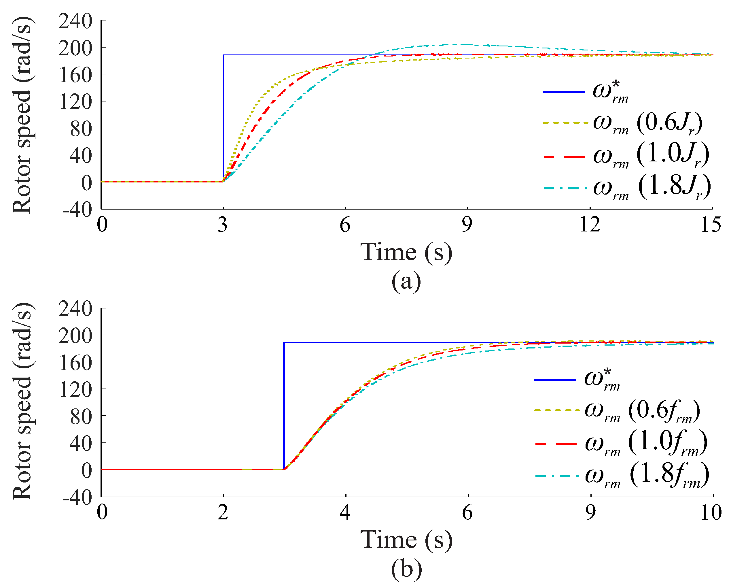
7.1.2. System Performance Analysis Assuming Variations in Armature Speed

Figure 16 shows the effect of armature speed variation on rotor speed dynamic behavior. In addition, the relationship between armature speed and angular frequency of the armature and rotor currents is also presented. According to Figure 16a, the variations in the mechanical speed of the EFR armature shown in Figure 16b result in small oscillations in rotor speed. However, these oscillations quickly converge to the reference value, so that rotor speed remains constant during system operation. As indicated in Figure 16b,c, a change in the mechanical speed of the EFR armature results in a proportional change in the frequency of the armature currents, so that the absolute angular speed of the armature rotating field given in (1) always remains constant. In this case, the frequency of the rotor currents, which corresponds to the slip speed described in (2), also remains constant during variations in the armature rotating speed, as shown in Figure 16d.

Figure 16. Relationship between mechanical speed and angular frequency in the EFR device: (a) EFR rotor speed, (b) EFR armature speed, (c) armature current frequency and (d) Rotor current frequency.

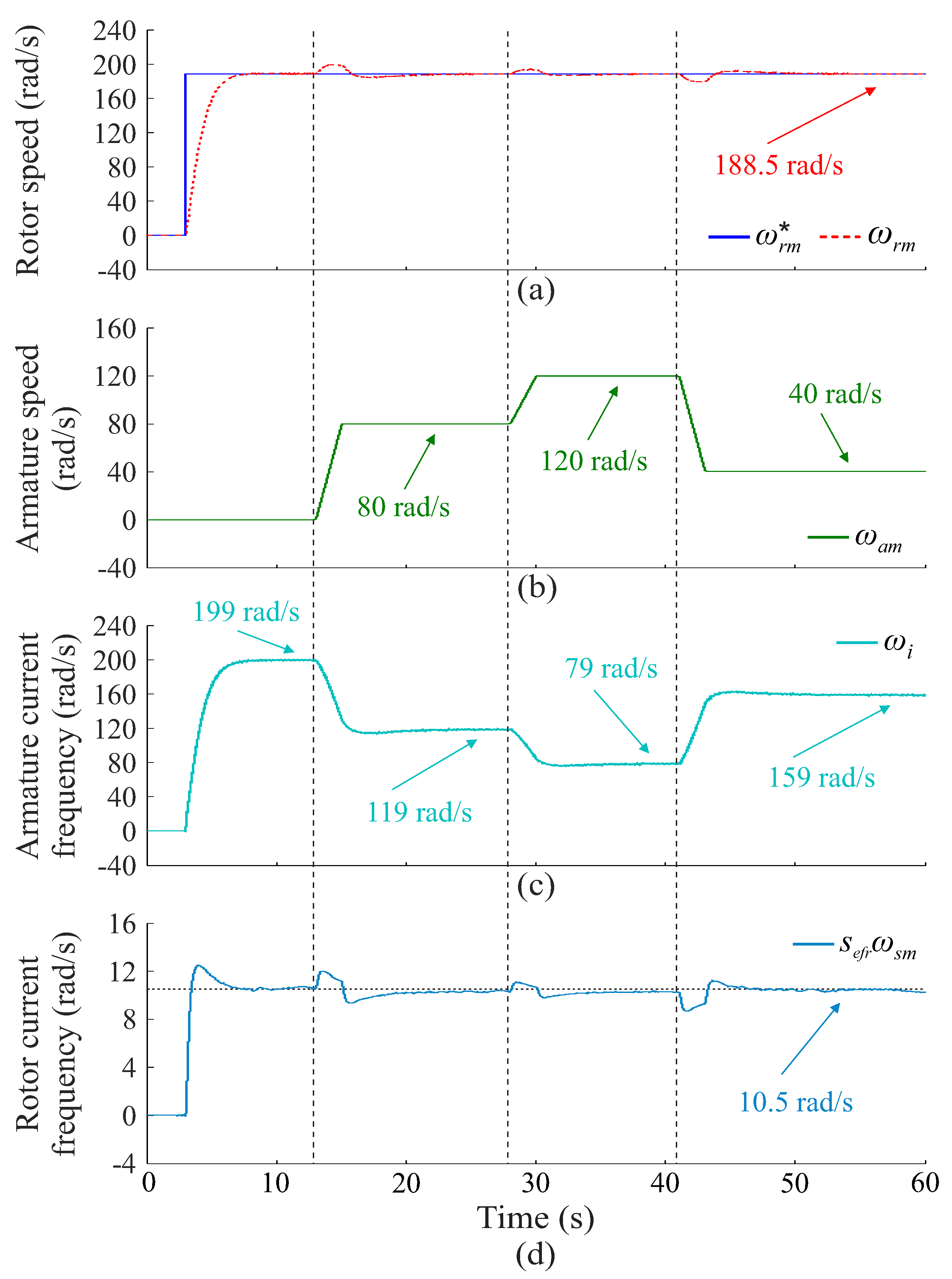
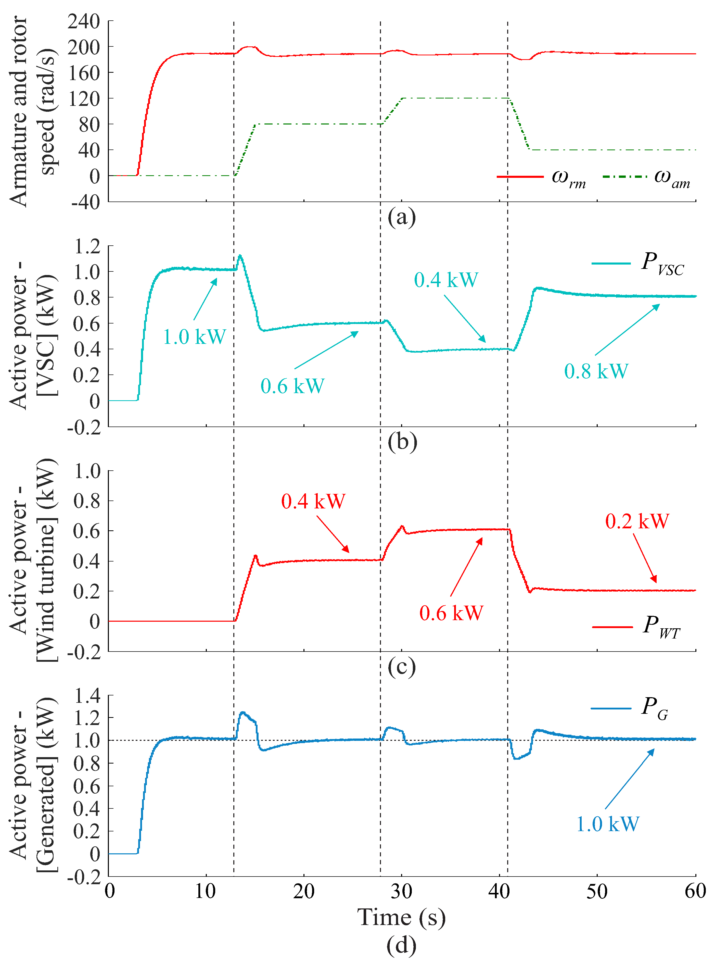
7.1.3. System Power-Sharing Analysis

Figure 17 shows power-sharing in the EFR-based system during armature speed variations. According to Figure 17a, in the interval from 3 to 13 s, the EFR rotor operates at a speed equal to $188.5$ rad/s, while the armature shaft is in repose. In this interval, the power supplied by the primary source of the VSC is equal to the generated power of 1 kW (100%), as shown in Figure 17b,d, while the power supplied by the wind turbine is equal to zero (0%) as shown in Figure 17c. In the interval of 13 to 28 s, the armature speed reaches 80 rad/s, which results in the reduction of the power supplied by the VSC to $0.6$ kW (60%) and in increasing the power supplied by the wind turbine to $0.4$ kW (40%), as shown in Figure 17b,c, respectively. When the armature speed reaches 120 rad/s, which occurs in the interval of 28 to 41 s, the power supplied by the VSC and the wind turbine are $0.4$ kW (40%) and $0.6$ kW (60%), respectively. Finally, for $t>41$ s, the armature speed decreases to 40 rad/s, which corresponds to a power supplied by the VSC of $0.8$ kW (80%) and a power supplied by the wind turbine of $0.2$ kW (20%). Based on these results, it is possible to share between the power supplied by the VSC and the wind turbine so that the power generated is always constant, as shown in Figure 17d. Therefore, the EFR-based system allows for implementation of a hybrid generation system with two energy sources providing the resulting power to the power grid or to an isolated load.

Figure 17. Power-sharing in the EFR-based system: (a) armature end rotor speed, (b) VSC active power, (c) wind turbine active power and (d) generated active power.

7.2. Experimental Results

To demonstrate the validity of the proposed performance analysis, experimental results were obtained using a laboratory setup to emulate the EFR-based system, as shown in Figure 18. In the experimental platform, a DC motor was used to emulate wind turbine behavior, as indicated in Figure 18c. Furthermore, the control algorithm was executed using a fast prototyping system DSP-TMS320f28335 with a sampling time of 100 $\mathsf{\mu }$s. The measurement of instantaneous voltage and current values was performed using hall-effect sensors LV20-P and LAH25-NP, respectively.

Figure 18. Experimental platform: (a) block diagram, (b) layout of laboratory equipment and (c) prototype machinery.

The experimental assays employed the same reference values for flux and speed control used in the simulation assays, which correspond to $1.2$ Wb and $188.5$ rad/s, respectively. Figure 19 shows the speed controller dynamic response. In addition, the generator a-phase armature voltage is also presented. According to Figure 19a, the rotor speed converges to the reference value without percent overshoot and with a transient response compatible with the design criteria adopted for the speed controller, as shown in Table 4. At $t=28$ s, the rotational movement of the EFR armature is started. In this case, the DC motor that emulates the wind turbine is driven in order to establish an armature rotation speed equal to 50 rad/s (Figure 19a), approximately. According to Figure 19b, the amplitude and frequency of the voltage delivered to the resistive load remains constant different armature speeds, which is desired during system operation.

Figure 19. Experimental results for performance analysis of the EFR-based system: (a) rotor and armature speed and (b) load voltage.

Table 4. Comparison between simulation and experimental results.

		Simulation	Experimental
	Design Criteria	Values Obtained	Values Obtained
Speed Controller	Settling time $T_{s2\%}⩽4$ s	$3.8$ s	4 s
	Percent overshoot $\%OS⩽5$%	0	0

8. Conclusions

This paper presented a performance analysis applied to an electromagnetic frequency regulator employed in distributed generation systems based on wind sources. Analyzes based on transient and steady-state response specifications indicated the influence of the variation of electromagnetic frequency regulator device parameters on its dynamic behavior. The paper also presented the design methodology of the system’s controllers and a sensitivity analysis of the closed-loop poles which were validated through simulation and experimental results. This work serves as a complement to the previous related works and contributes to the proper operation of the electromagnetic frequency regulator device in distributed generation systems, since the control strategy has a great influence on the system dynamic performance. In addition, the electromagnetic frequency regulator device also allows the implementation of a hybrid generation system with the integration of photovoltaic energy to supply the power converter. Future work is needed to evaluate the electromagnetic frequency regulator dynamic behavior operating with more robust control strategies in relation to parametric variations and perturbations.

References

- Akella, A.K.; Saini, R.P.; Sharma, M.P. Social, economical and environmental impacts of renewable energy systems. Renew. Energy 2009, 34, 390–396. [Google Scholar] [CrossRef]
- Duan, Y.; Harley, R.G. Present and future trends in wind turbine generator designs. IEEE Power Electron. Mach. Wind Appl. 2009, 1, 1–6. [Google Scholar]
- Global Wind Energy Council. Global Wind Report 2021. 2021. Available online: https://gwec.net/global-wind-report-2021/ (accessed on 4 May 2021).
- Alhmoud, L.; Wang, B. A review of the state-of-the-art in wind-energy reliability analysis. Renew. Sustain. Energy Rev. 2018, 81, 1643–1651. [Google Scholar] [CrossRef]
- Polinder, H.; Pijl, F.F.A.V.D.; Vilder, G.D.; Tavner, P.J. Comparison of direct-drive and geared generator concepts for wind turbines. IEEE Trans. Energy Convers. 2006, 21, 725–733. [Google Scholar] [CrossRef] [Green Version]
- Herbet, G.J.; Iniyan, S.; Sreevalsan, E.; Rajapandian, S. A review of wind energy technologies. Renew. Sustain. Energy Rev. 2007, 11, 1117–1145. [Google Scholar] [CrossRef]
- Thresher, R.; Robinson, M.; Veers, P. To capture the wind. IEEE Power Energy Mag. 2007, 5, 34–46. [Google Scholar] [CrossRef]
- Yaramasu, V.; Wu, B.; Sen, P.C.; Kouro, S.; Narimani, M. High-power wind energy conversion systems: State-of-the-art and emerging technologies. Proc. IEEE 2015, 103, 740–788. [Google Scholar] [CrossRef]
- Perez, J.M.P.; Marquez, F.P.G.; Tobias, A.; Papaelias, M. Wind turbine reliability analysis. Renew. Sustain. Energy Rev. 2013, 23, 463–472. [Google Scholar] [CrossRef]
- Mckenna, R.; Leye, P.O.V.D.; Fichtner, W. Key challenges and prospects for large wind turbines. Renew. Sustain. Energy Rev. 2016, 53, 1212–1221. [Google Scholar] [CrossRef]
- Vitor Silva, P.; Ferreira Pinheiro, R.; Ortiz Salazar, A.; do Santos Junior, L.P.; de Azevedo, C.C. A Proposal for a New Wind Turbine Topology Using an Electromagnetic Frequency Regulator. IEEE Lat. Am. Trans. 2015, 13, 989–997. [Google Scholar] [CrossRef]
- Silva, P.V.; Pinheiro, R.F.; Salazar, A.O.; Fernandes, J.D. Performance analysis of a new system for speed control in wind turbines. Renew. Energy Power Qual. J. 2015, 1, 455–460. [Google Scholar] [CrossRef]
- Silva, P.V.; Pinheiro, R.F.; Salazar, A.O.; Júnior, L.P.S.; Fernandes, J.D. A New System for Speed Control in Wind Turbines using the Electromagnetic Frequency Regulator. Eletrônica Potência 2015, 20, 254–262. [Google Scholar] [CrossRef] [Green Version]
- Ramos, T.; Júnior, M.M.; Pinheiro, R.; Medeiros, A. Slip Control of a Squirrel Cage Induction Generator Driven by an Electromagnetic Frequency Regulator to Achieve the Maximum Power Point Tracking. Energies 2019, 12, 2100. [Google Scholar] [CrossRef] [Green Version]
- Da Silva, J.C.L.; Ramos, T.; Júnior, M.F.M. Modeling and Harmonic Impact Mitigation of Grid-Connected SCIG Driven by an Electromagnetic Frequency Regulator. Energies 2021, 14, 4524. [Google Scholar] [CrossRef]
- Do Nascimento, T.F.; Nunes, E.A.F.; Salazar, A.O. Modeling and Controllers Design for an Electromagnetic Frequency Regulator Applied to Wind Systems. In Proceedings of the 2021 Brazilian Power Electronics Conference (COBEP), João Pessoa, Brazil, 7–10 November 2021; pp. 1–8. [Google Scholar]
- Blasko, V. Analysis of a hybrid PWM based on modified space-vector and triangle-comparison methods. IEEE Trans. Ind. Appl. 1997, 33, 756–764. [Google Scholar] [CrossRef]
- De Doncker, R.W.; Novotny, D.W. The universal field oriented controller. IEEE Trans. Ind. Appl. 1994, 30, 92–100. [Google Scholar] [CrossRef]
- Jacobina, C.B.; Lima, A.M.N. Estratégias de Controle Para Sistemas de Acionamento Com Máquina Assíncrona. SBA Controle Automação 1996, 7, 15–28. [Google Scholar]
- Nise, N.S. Control Systems Engineering, 6th ed.; John Wiley & Sons, Inc.: Hoboken, NJ, USA, 2011. [Google Scholar]
- Li, Y.W. Control and Resonance Damping of Voltage-Source and Current-Source Converters with LC Filters. IEEE Trans. Ind. Electron. 2009, 56, 1511–1521. [Google Scholar]
- Kim, K.; Van, T.L.; Lee, D.; Song, S.; Kim, E. Maximum Output Power Tracking Control in Variable-Speed Wind Turbine Systems Considering Rotor Inertial Power. IEEE Trans. Ind. Electron. 2013, 60, 3207–3217. [Google Scholar] [CrossRef]
Publisher’s Note: MDPI stays neutral with regard to jurisdictional claims in published maps and institutional affiliations. |
© 2022 by the authors. Licensee MDPI, Basel, Switzerland. This article is an open access article distributed under the terms and conditions of the Creative Commons Attribution (CC BY) license (https://creativecommons.org/licenses/by/4.0/).