
Optimization of Well Control during Gas Flooding Using the Deep-LSTM-Based Proxy Model: A Case Study in the Baoshaceng Reservoir, Tarim, China

 ,
,
Abstract
:1. Introduction
2. Materials and Methods
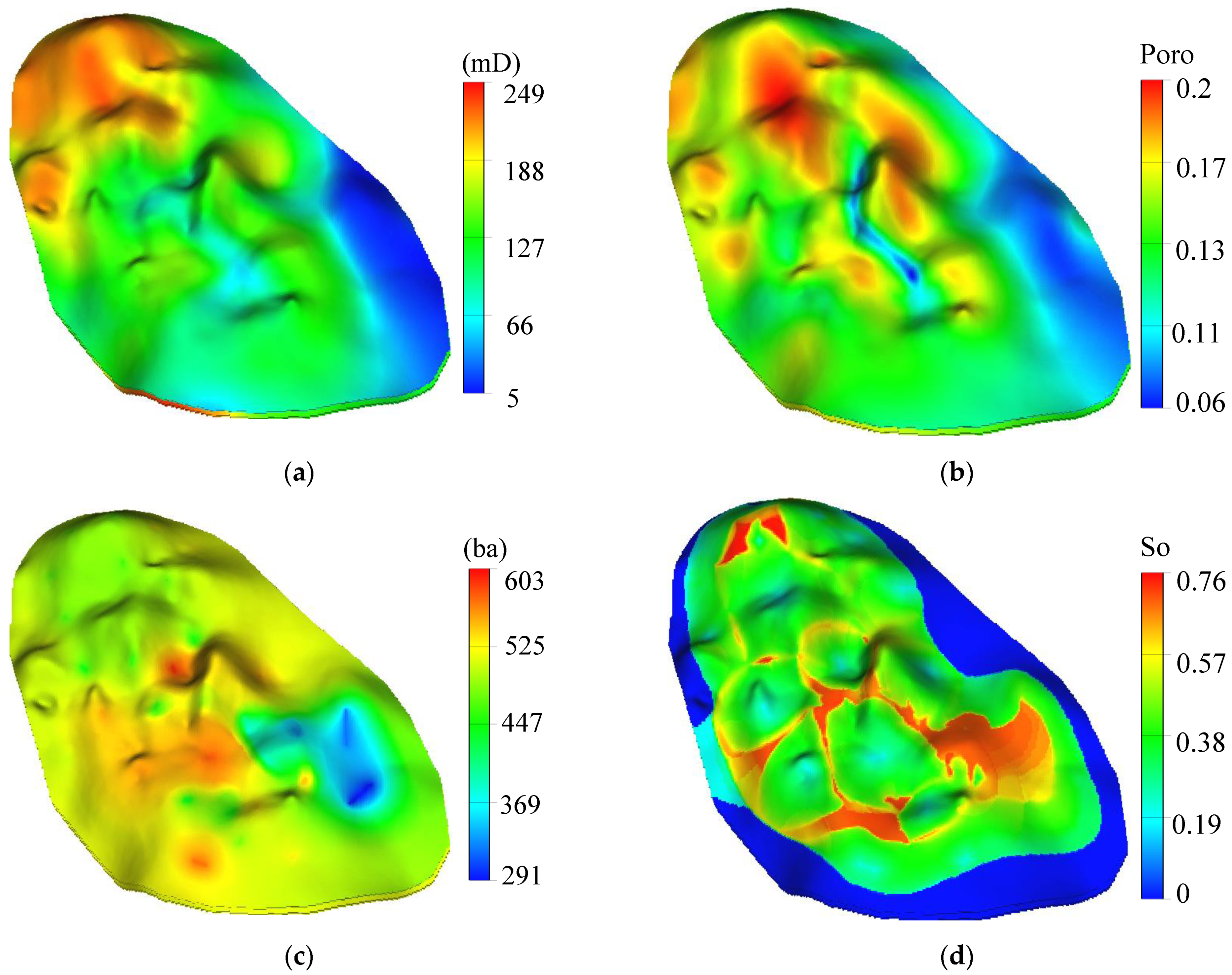
2.1. Background of the Baoshaceng Reservoir
2.2. Sample Construction
2.3. Development of the Deep-LSTM Proxy Model
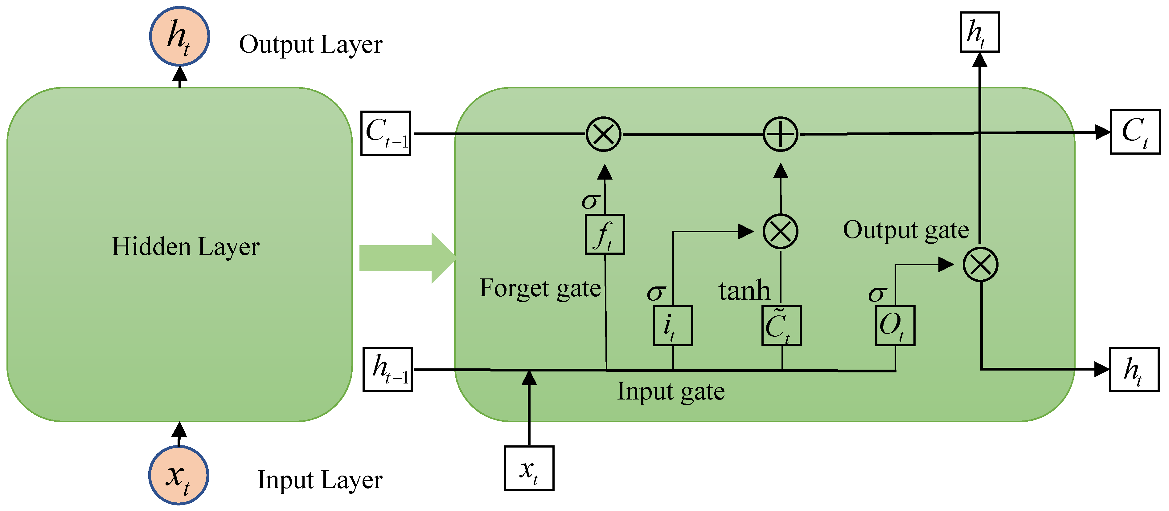
2.3.1. Basics of the Deep-LSTM
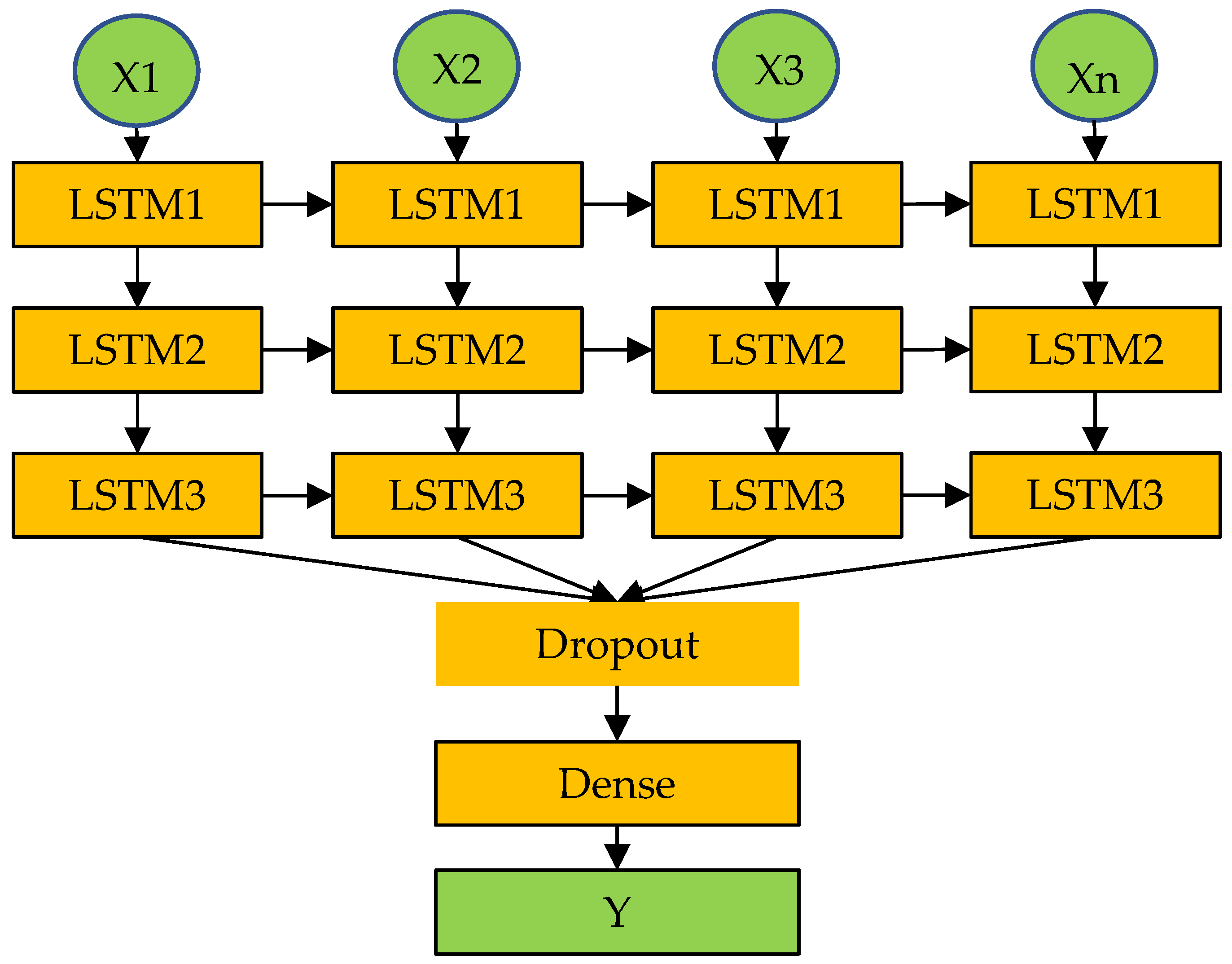
2.3.2. Construction of the Deep-LSTM Proxy Model
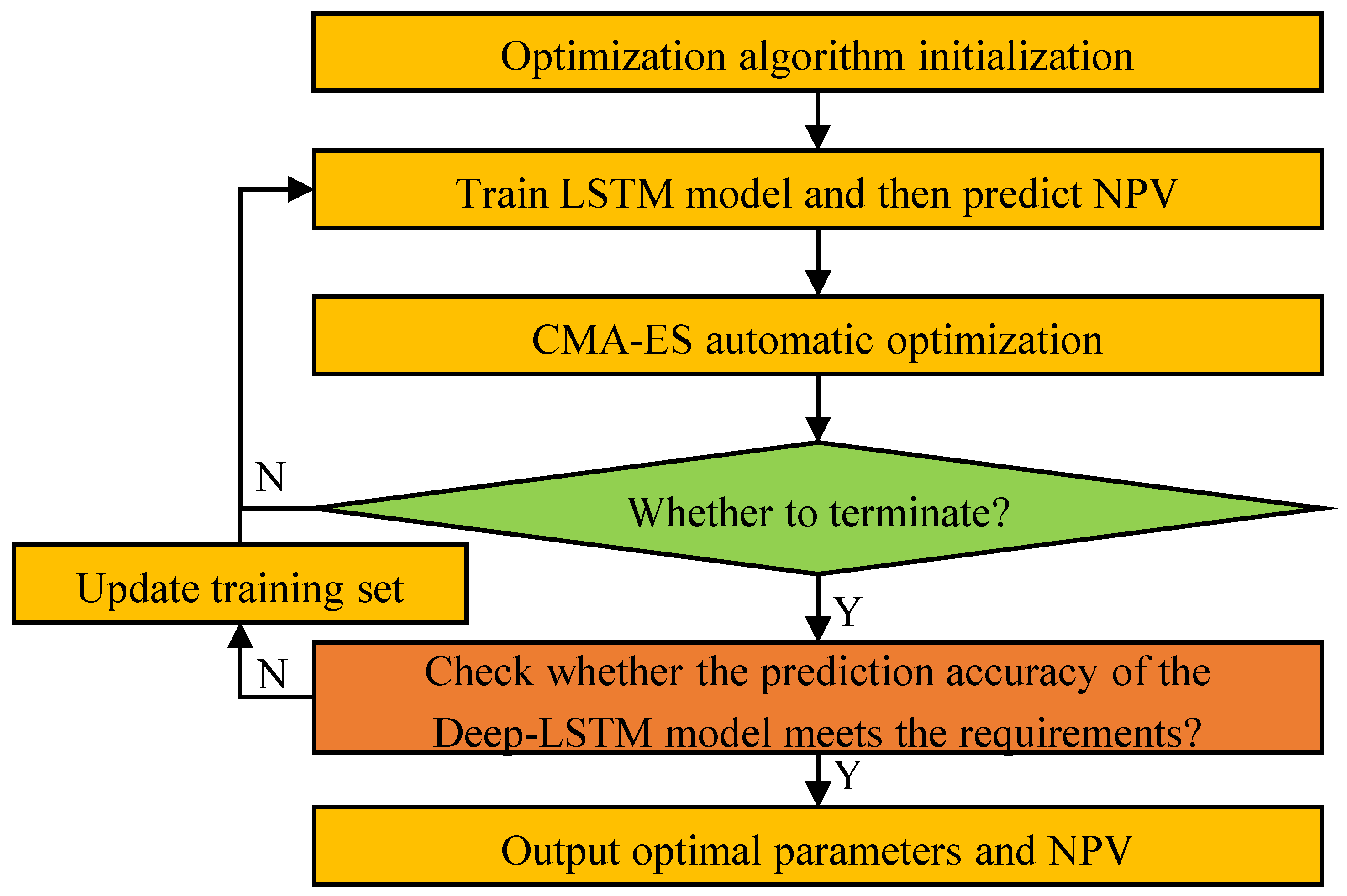
2.4. Optimization of the Well Control Parameters for Gas Flooding
- Step 1: Initialize the optimization algorithm and the optimization variables;
- Step 2: Train the Deep-LSTM model and then predict NPV;
- Step 3: Automatic optimization of CMA-ES algorithm;
- Step 4: Determine whether the termination condition is reached;
- Step 5: If the prediction accuracy of the Deep-LSTM model meets the requirements, output optimal well control parameters and NPV; otherwise, repeat from Step 2 to Step 4 (e.g., update the training set, retrain the model, restart the optimization algorithm).
3. Results and Discussion
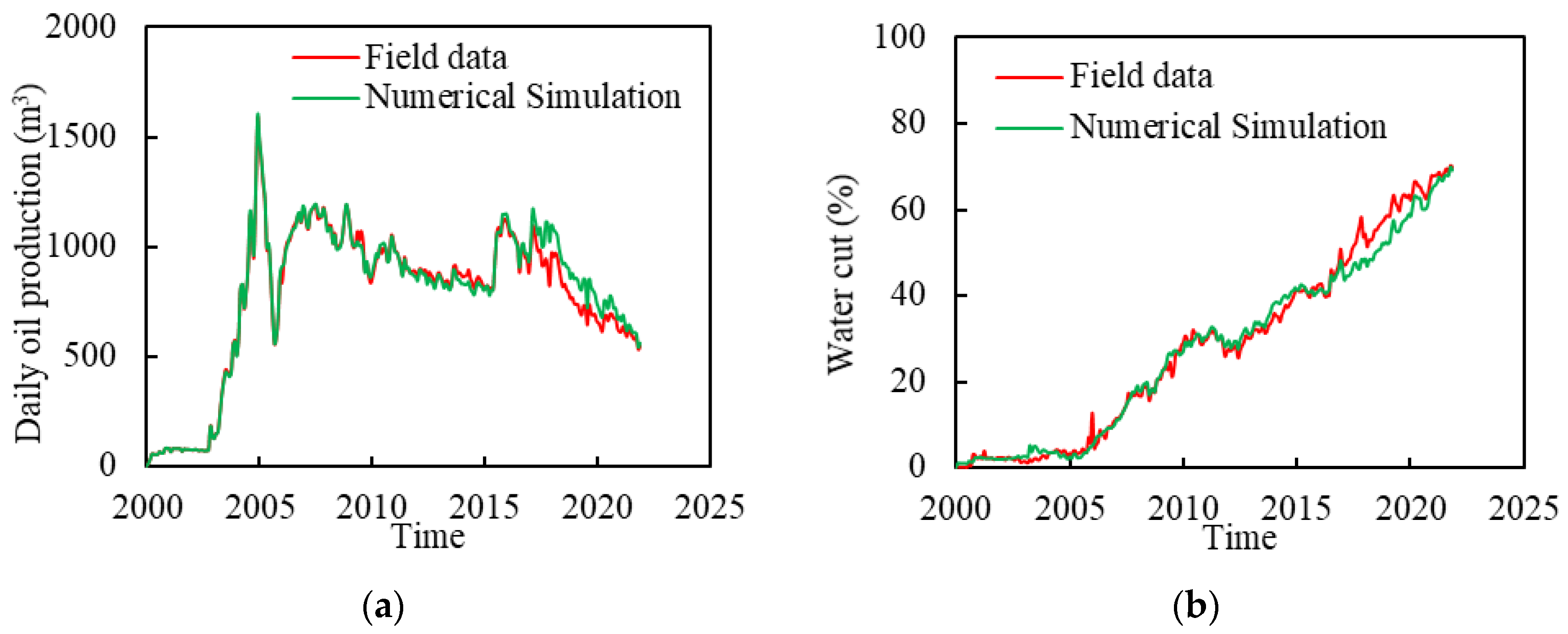
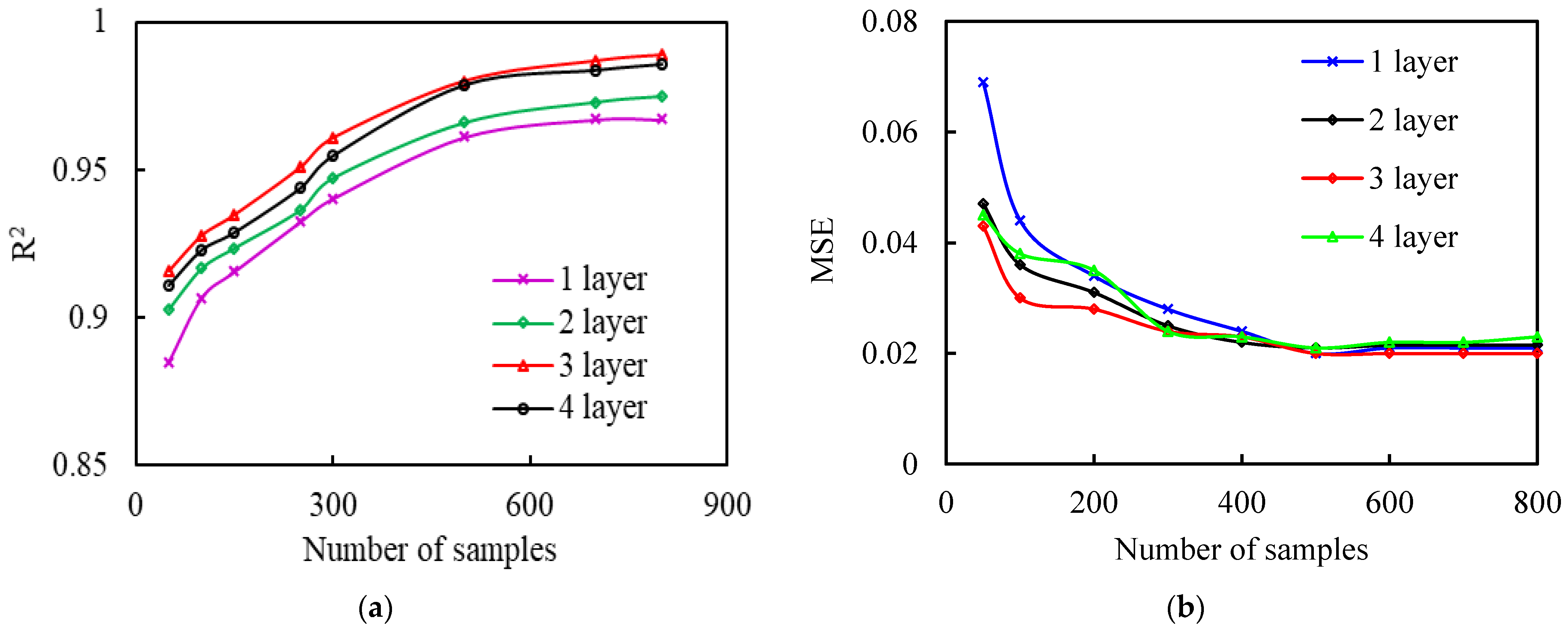
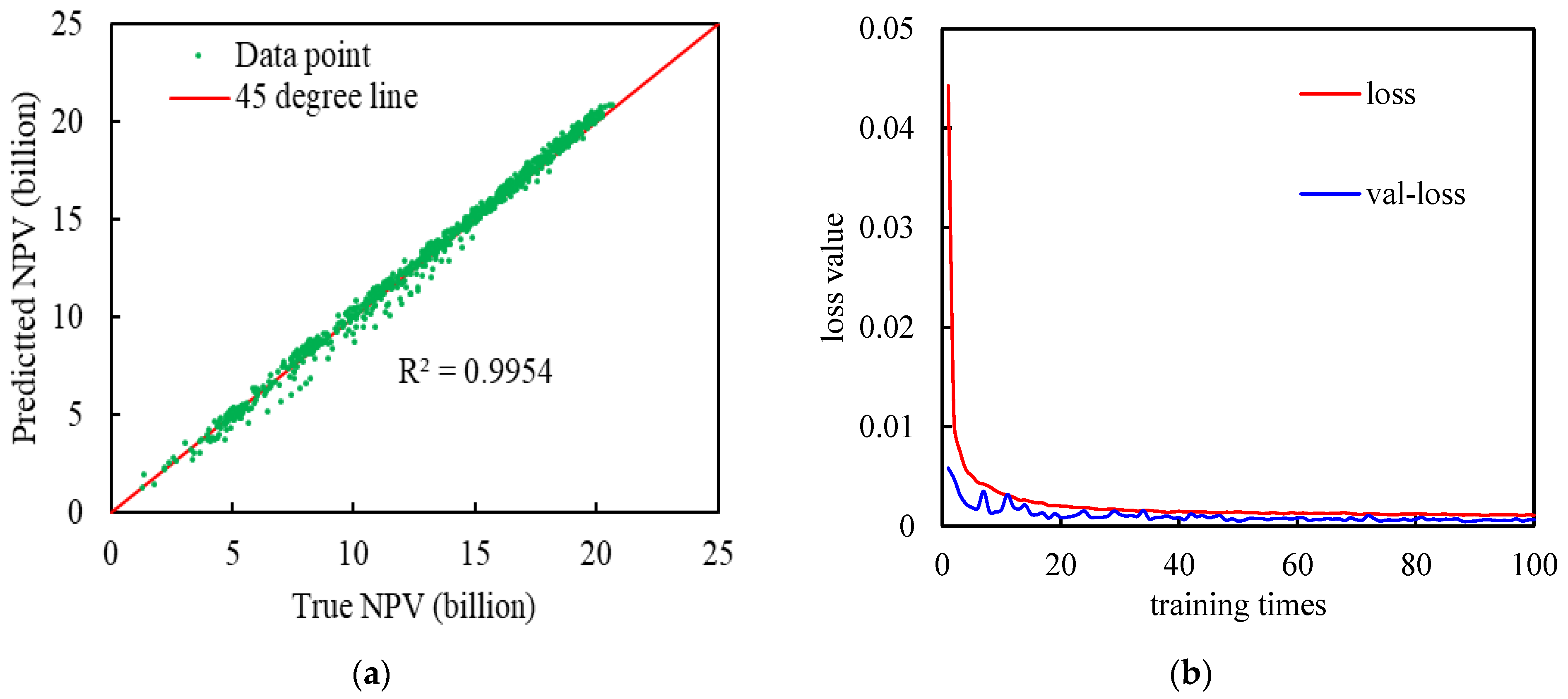
3.1. Development of the Proxy Model
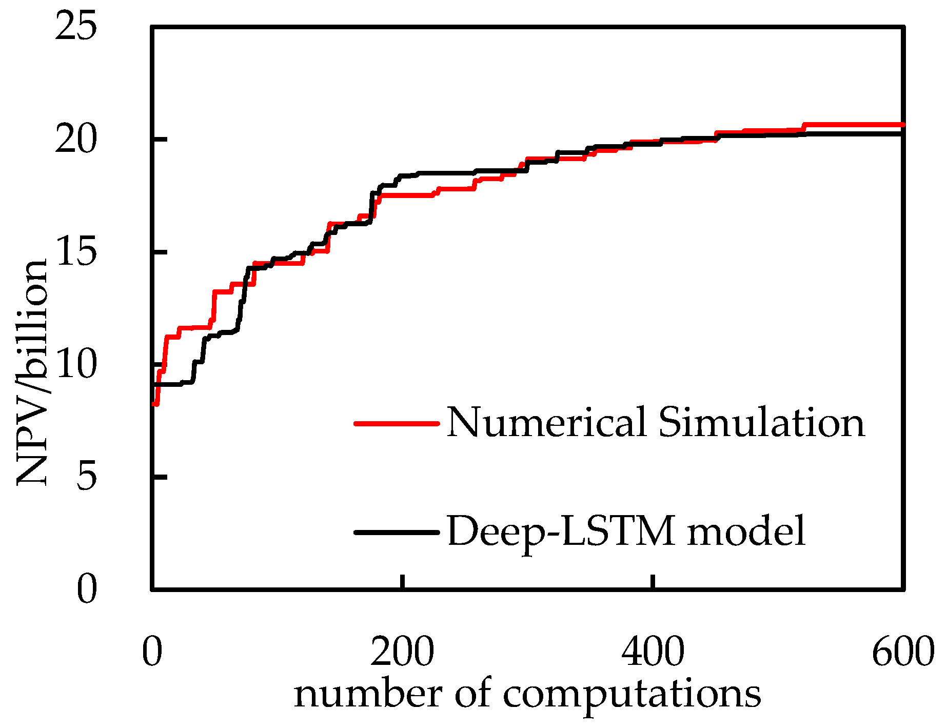
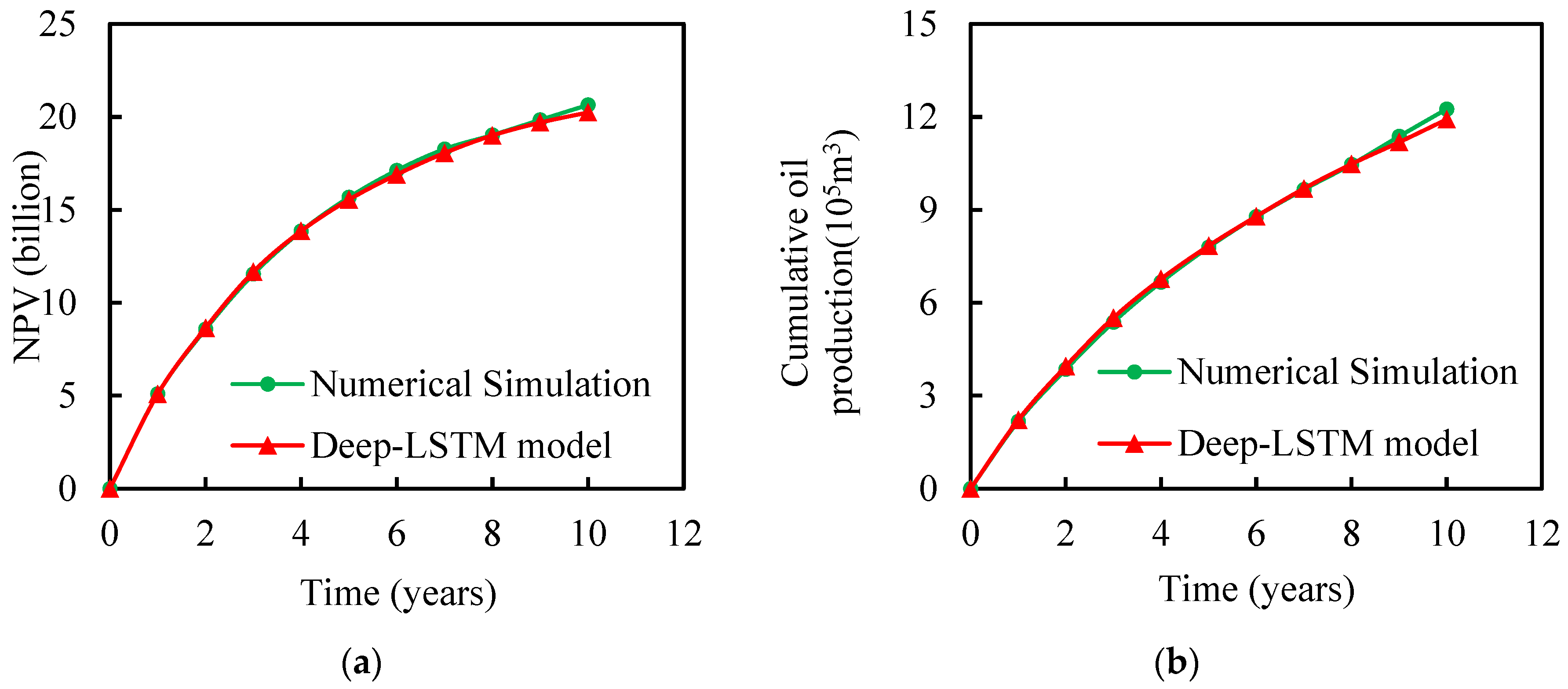
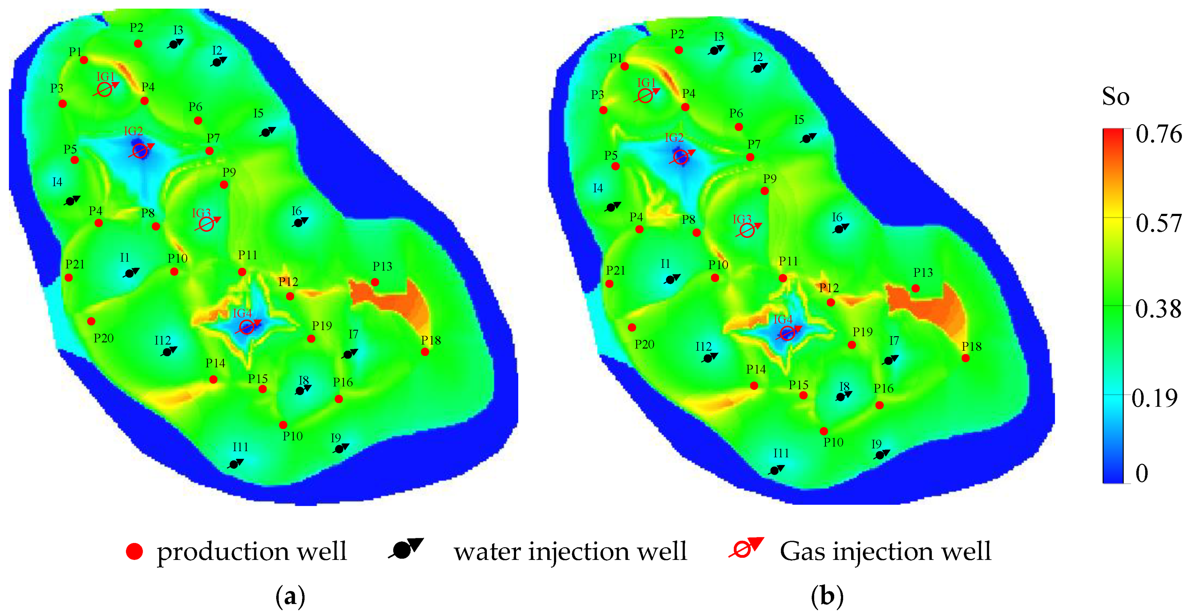
3.2. Optimization of the Well Control Parameters
4. Conclusions
Author Contributions
Funding
Institutional Review Board Statement
Informed Consent Statement
Data Availability Statement
Conflicts of Interest
References
- Sheng, J.J. Enhanced oil recovery in shale reservoirs by gas injection. J. Nat. Gas Sci. Eng. 2015, 22, 252–259. [Google Scholar] [CrossRef] [Green Version]
- Qi, Z.; Liu, T.; Xi, C.; Zhang, Y.; Shen, D.; Mu, H.; Dong, H.; Zheng, A.; Yu, K.; Li, X. Status Quo of a CO2-Assisted Steam-Flooding Pilot Test in China. Geofluids 2021, 2021, 9968497. [Google Scholar] [CrossRef]
- Li, X.; Wang, S.; Yuan, B.; Chen, S. Optimal Design and Uncertainty Assessment of CO2 WAG Operations: A Field Case Study. In Proceedings of the SPE Improved Oil Recovery Conference, Tulsa, OK, USA, 14–18 April 2018. [Google Scholar]
- Ghedan, S.G. Global laboratory experience of CO2-EOR flooding. In Proceedings of the SPE/EAGE Reservoir Characterization and Simulation Conference, Abu Dhabi, United Arab Emirates, 19–21 October 2009. [Google Scholar]
- Chen, B.; Reynolds, A.C. Ensemble-based optimization of the water-alternating-gas-injection process. SPE J. 2016, 21, 0786–0798. [Google Scholar] [CrossRef]
- Liu, S.; Agarwal, R.; Sun, B.; Wang, B.; Li, H.; Xu, J.; Fu, G. Numerical simulation and optimization of injection rates and wells placement for carbon dioxide enhanced gas recovery using a genetic algorithm. J. Clean. Prod. 2021, 280, 124512. [Google Scholar] [CrossRef]
- Chakra, N.C.; Song, K.-Y.; Gupta, M.M.; Saraf, D.N. An innovative neural forecast of cumulative oil production from a petroleum reservoir employing higher-order neural networks (HONNs). J. Pet. Sci. Eng. 2013, 106, 18–33. [Google Scholar] [CrossRef]
- Wang, S.; Chen, Z.; Chen, S. Applicability of deep neural networks on production forecasting in Bakken shale reservoirs. J. Pet. Sci. Eng. 2019, 179, 112–125. [Google Scholar] [CrossRef]
- Gu, J.; Liu, W.; Zhang, K.; Zhai, L.; Zhang, Y.; Chen, F. Reservoir production optimization based on surrograte model and differential evolution algorithm. J. Pet. Sci. Eng. 2021, 205, 108879. [Google Scholar] [CrossRef]
- Wang, S.; Qin, C.; Feng, Q.; Javadpour, F.; Rui, Z. A framework for predicting the production performance of unconventional resources using deep learning. Appl. Energy 2021, 295, 117016. [Google Scholar] [CrossRef]
- Hui, G.; Chen, S.; He, Y.; Wang, H.; Gu, F. Machine learning-based production forecast for shale gas in unconventional reservoirs via integration of geological and operational factors. J. Nat. Gas Sci. Eng. 2021, 94, 104045. [Google Scholar] [CrossRef]
- Huang, R.; Wei, C.; Wang, B.; Yang, J.; Xu, X.; Wu, S.; Huang, S. Well performance prediction based on Long Short-Term Memory (LSTM) neural network. J. Pet. Sci. Eng. 2022, 208, 109686. [Google Scholar] [CrossRef]
- Javadi, A.; Moslemizadeh, A.; Moluki, V.S.; Fathianpour, N.; Mohammadzadeh, O.; Zendehboudi, S. A Combination of Artificial Neural Network and Genetic Algorithm to Optimize Gas Injection: A Case Study for EOR Applications. J. Mol. Liq. 2021, 339, 116654. [Google Scholar] [CrossRef]
- Shields, M.D.; Zhang, J. The generalization of Latin hypercube sampling. Reliab. Eng. Syst. Saf. 2016, 148, 96–108. [Google Scholar] [CrossRef] [Green Version]
- Zhang, K.; Wang, Z.; Chen, G.; Zhang, L.; Yang, Y.; Yao, C.; Wang, J.; Yao, J. Training effective deep reinforcement learning agents for real-time life-cycle production optimization. J. Pet. Sci. Eng. 2022, 208, 109766. [Google Scholar] [CrossRef]
- Kim, J.; Lee, K.; Choe, J. Efficient and robust optimization for well patterns using a PSO algorithm with a CNN-based proxy model. J. Pet. Sci. Eng. 2021, 207, 109088. [Google Scholar] [CrossRef]
- Zaac, D.; Kang, Z.B.; Jian, H.; Dwac, D.; Ypac, D. Accelerating reservoir production optimization by combining reservoir engineering method with particle swarm optimization algorithm. J. Pet. Sci. Eng. 2022, 208, 109692. [Google Scholar]
- Bhanja, S.; Das, A. Impact of Data Normalization on Deep Neural Network for Time Series Forecasting. arXiv 2018, arXiv:1812.05519. [Google Scholar]
- Alom, M.Z.; Taha, T.M.; Yakopcic, C.; Westberg, S.; Sidike, P.; Nasrin, M.S.; Hasan, M.; Van Essen, B.C.; Awwal, A.A.; Asari, V.K. A state-of-the-art survey on deep learning theory and architectures. Electronics 2019, 8, 292. [Google Scholar] [CrossRef] [Green Version]
- Sherwani, F.; Ibrahim, B.; Asad, M.M. Hybridized classification algorithms for data classification applications: A review. Egypt. Inform. J. 2021, 22, 185–192. [Google Scholar] [CrossRef]
- DiPietro, R.; Hager, G.D. Deep learning: RNNs and LSTM. In Handbook of Medical Image Computing and Computer Assisted Intervention; Elsevier: Amsterdam, The Netherlands, 2020; pp. 503–519. [Google Scholar]
- Sagheer, A.; Kotb, M. Time series forecasting of petroleum production using deep LSTM recurrent networks. Neurocomputing 2019, 323, 203–213. [Google Scholar] [CrossRef]
- Bao, R.; He, Z.; Zhang, Z. Application of lightning spatio-temporal localization method based on deep LSTM and interpolation. Measurement 2022, 189, 110549. [Google Scholar] [CrossRef]
- Jais, I.K.M.; Ismail, A.R.; Nisa, S.Q. Adam optimization algorithm for wide and deep neural network. Knowl. Eng. Data Sci. 2019, 2, 41–46. [Google Scholar] [CrossRef]
- Nguyen, L.C.; Nguyen-Xuan, H. Deep learning for computational structural optimization. ISA Trans. 2020, 103, 177–191. [Google Scholar] [CrossRef] [PubMed]
- Liu, X.; Wu, J.; Chen, S. A Context-Based Meta-Reinforcement Learning Approach to Efficient Hyperparameter Optimization. Neurocomputing 2022, 478, 89–103. [Google Scholar] [CrossRef]
- Wu, J.; Chen, X.-Y.; Zhang, H.; Xiong, L.-D.; Lei, H.; Deng, S.-H. Hyperparameter optimization for machine learning models based on Bayesian optimization. J. Electron. Sci. Technol. 2019, 17, 26–40. [Google Scholar]
- Snoek, J.; Larochelle, H.; Adams, R.P. Practical bayesian optimization of machine learning algorithms. Adv. Neural Inf. Processing Syst. 2012, 28. Available online: https://arxiv.org/abs/1206.2944 (accessed on 1 February 2022).
- Eggensperger, K.; Feurer, M.; Hutter, F.; Bergstra, J.; Snoek, J.; Hoos, H.; Leyton-Brown, K. Towards an empirical foundation for assessing bayesian optimization of hyperparameters. In Proceedings of the NIPS workshop on Bayesian Optimization in Theory and Practice, Lake Tahoe, NV, USA, 10 December 2013. [Google Scholar]
- Victoria, A.H.; Maragatham, G. Automatic tuning of hyperparameters using Bayesian optimization. Evol. Syst. 2021, 12, 217–223. [Google Scholar] [CrossRef]
- Rios, L.M.; Sahinidis, N.V. Derivative-free optimization: A review of algorithms and comparison of software implementations. J. Glob. Optim. 2013, 56, 1247–1293. [Google Scholar] [CrossRef] [Green Version]
- Hansen, N.; Müller, S.D.; Koumoutsakos, P. Reducing the time complexity of the derandomized evolution strategy with covariance matrix adaptation (CMA-ES). Evol. Comput. 2003, 11, 1–18. [Google Scholar] [CrossRef]
- KUANG, L.; He, L.; Yili, R.; Kai, L.; Mingyu, S.; Jian, S.; Xin, L. Application and development trend of artificial intelligence in petroleum exploration and development. Pet. Explor. Dev. 2021, 48, 1–14. [Google Scholar] [CrossRef]

| Parameters | Lower Sampling Limit | Upper Sampling Limit |
|---|---|---|
| Gas injection timing (days) | 0 | 120 |
| Gas injection rate (m3/d) | 0 | 120,000 |
| Total gas injection (108 m3) | 0 | 4 |
| Water injection rate (m3/d) | 0 | 150 |
| Liquid production rate (m3/d) | 0 | 150 |
| Parameters | Value |
|---|---|
| Gas injection cost (RMB/m3) | 1.3 |
| Water injection cost (RMB/m3) | 30 |
| Water treatment cost (RMB/m3) | 10 |
| Oil sale price (RMB/m3) | 2800 |
| Gas sale price (RMB/m3) | 0.9 |
| Annual discount rate | 10 |
| Parameter | Type |
|---|---|
| RAM | 16G |
| GPU | NVIDIA GTX 1060 |
| CPU | Intel i7 10875H@2.30 GHz |
| Computer system | Windows10 |
| Deep learning environment | TensorFlow |
| Parameters | Range | Optimal Parameters |
|---|---|---|
| Learning rate | 0.0001~0.1 | 0.001 |
| Batch size | 20~100 | 32 |
| The number of neurons in the first layer | 10~200 | 24 |
| The number of neurons in the second layer | 10~200 | 48 |
| The number of neurons in the third layer | 10~200 | 60 |
| Loss function value(Dropout) | 0.05~0.5 | 0.2 |
| Epoch | 10~200 | 100 |
| Constraint Type | Constraint Variables | Constraint Expression |
|---|---|---|
| Inequality Boundary Condition Constraints | Gas injection timing | |
| Gas injection rate | ||
| Total gas injection | ||
| Liquid production rate | ||
| Water injection speed |
| Method | MSE | R2 |
|---|---|---|
| Deep-LSTM | 0.018 | 0.9954 |
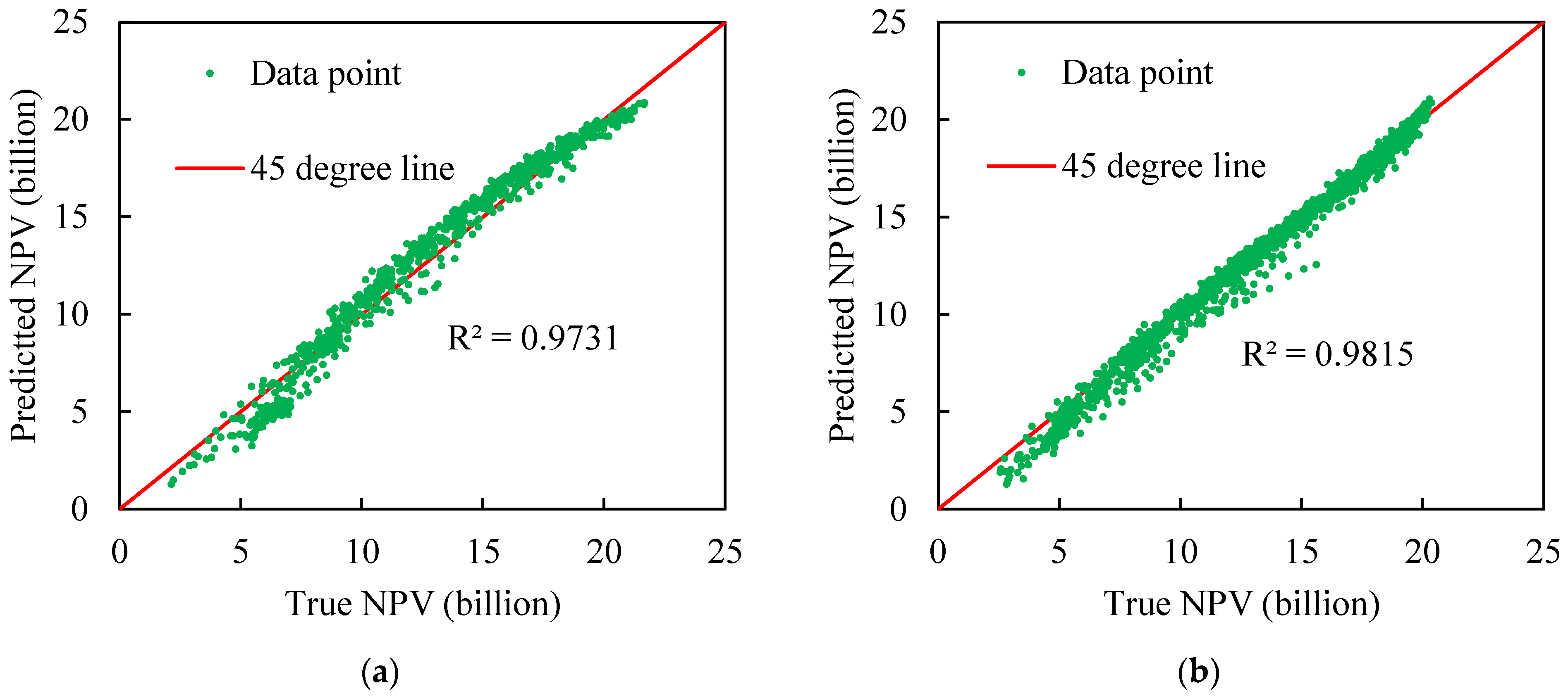
| FCNN | 0.059 | 0.9815 |
| XGBoost | 0.081 | 0.9731 |
| Optimization Parameters | Optimization Variables | Numerical Simulation | Deep-LSTM Model |
|---|---|---|---|
| gas injection start time (days) | It1 | 3365 | 3482 |
| It2 | 1 | 1 | |
| It3 | 3495 | 3330 | |
| It4 | 1111 | 954 | |
| gas injection rate (m3/d) | Ivg1 | 51,681.95 | 63,797.47 |
| Ivg2 | 114,304.78 | 115,261.37 | |
| Ivg3 | 95,569.58 | 88,207.42 | |
| Ivg4 | 87,742.34 | 89,058.18 | |
| gas injection volume (m3) | Icg1 | 368,426.22 | 236,419.96 |
| Icg2 | 193,615,238.47 | 144,773,030.62 | |
| Icg3 | 65,753,357.66 | 42,146,090.84 | |
| Icg4 | 55,483,180.47 | 57,906,751.61 |
| Water Injection Rate (m3/d) | Ivw1 | Ivw2 | Ivw3 | Ivw4 | Ivw5 | Ivw6 |
|---|---|---|---|---|---|---|
| Numerical simulation | 150.00 | 138.61 | 150.00 | 148.44 | 145.96 | 124.09 |
| Deep-LSTM model | 150.00 | 134.56 | 148.20 | 149.18 | 150.00 | 125.27 |
| Water Injection Rate (m3/d) | Ivw7 | Ivw8 | Ivw9 | Ivw10 | Ivw11 | Ivw12 |
| Numerical simulation | 100.54 | 65.26 | 56.00 | 98.66 | 140.36 | 142.38 |
| Deep-LSTM model | 136.31 | 77.60 | 65.32 | 91.25 | 146.33 | 1355.60 |
| Production Well Rate (m3/d) | P1 | P2 | P3 | P4 | P5 | P6 | P7 | P8 | P9 | P10 | P11 |
|---|---|---|---|---|---|---|---|---|---|---|---|
| Numerical simulation | 149 | 122.3 | 142 | 150.1 | 83.5 | 150.1 | 150.1 | 124.1 | 150.1 | 149.7 | 85.5 |
| Deep-LSTM model | 142.5 | 139 | 130.1 | 139 | 77 | 150.1 | 143.7 | 119 | 143.3 | 135 | 88.2 |
| Production Well Rate (m3/d) | P12 | P13 | P14 | P15 | P16 | P17 | P18 | P19 | P20 | P21 | |
| Numerical simulation | 108.1 | 98 | 91.6 | 132.8 | 73.9 | 142.6 | 69.1 | 1 | 57.9 | 120.2 | |
| Deep-LSTM model | 100.1 | 109.7 | 82.5 | 142.0 | 66.1 | 145 | 70 | 1 | 59 | 128.8 |
| Methods | NPV (Billion) | Cumulative Oil (105 m3) | CPU Time |
|---|---|---|---|
| Numerical simulation | 20.65 | 12.25 | 345.38 h |
| Deep-LSTM | 20.24 | 11.92 | 5 h 42 min |
| Error (%) | 2.1 | 2.7 | / |
Publisher’s Note: MDPI stays neutral with regard to jurisdictional claims in published maps and institutional affiliations. |
© 2022 by the authors. Licensee MDPI, Basel, Switzerland. This article is an open access article distributed under the terms and conditions of the Creative Commons Attribution (CC BY) license (https://creativecommons.org/licenses/by/4.0/).
Share and Cite
Feng, Q.; Wu, K.; Zhang, J.; Wang, S.; Zhang, X.; Zhou, D.; Zhao, A. Optimization of Well Control during Gas Flooding Using the Deep-LSTM-Based Proxy Model: A Case Study in the Baoshaceng Reservoir, Tarim, China. Energies 2022, 15, 2398. https://doi.org/10.3390/en15072398
Feng Q, Wu K, Zhang J, Wang S, Zhang X, Zhou D, Zhao A. Optimization of Well Control during Gas Flooding Using the Deep-LSTM-Based Proxy Model: A Case Study in the Baoshaceng Reservoir, Tarim, China. Energies. 2022; 15(7):2398. https://doi.org/10.3390/en15072398
Chicago/Turabian StyleFeng, Qihong, Kuankuan Wu, Jiyuan Zhang, Sen Wang, Xianmin Zhang, Daiyu Zhou, and An Zhao. 2022. "Optimization of Well Control during Gas Flooding Using the Deep-LSTM-Based Proxy Model: A Case Study in the Baoshaceng Reservoir, Tarim, China" Energies 15, no. 7: 2398. https://doi.org/10.3390/en15072398
APA StyleFeng, Q., Wu, K., Zhang, J., Wang, S., Zhang, X., Zhou, D., & Zhao, A. (2022). Optimization of Well Control during Gas Flooding Using the Deep-LSTM-Based Proxy Model: A Case Study in the Baoshaceng Reservoir, Tarim, China. Energies, 15(7), 2398. https://doi.org/10.3390/en15072398