Detailed Assessment of Modulation Strategies for Hexverter–Based Modular Multilevel Converters

Abstract

Modular multilevel converters are playing a key role in the present and future development of topologies for medium–to–high–power applications. Among this category of power converters, there is a direct AC–AC modular multilevel converter called “Hexverter”, which is well suited to connect three–phase AC systems operating at different frequencies. This topology is the subject of study in this manuscript. The complete Hexverter system is composed of an Hexverter power converter and several control layers, namely, a “virtual $V_{\mathrm{C}}^2$ controller”, a branch current controller in a two–frequency $dq$ reference frame, a modulator, and a voltage balancing algorithm. The paper presents a thorough description and analysis of the entire Hexverter system, providing research contributions in three key aspects: (i) modeling and control in a unified two–frequency $dq$ framework; (ii) developing a “virtual $V_{\mathrm{C}}^2$ controller” to dynamically account for Hexverter’s active power losses allowing to achieve active power balance on the fly; and (iii) a comparative evaluation of modulation strategies (nearest level control and phase disposition–sinusoidal pulse width modulation). To this end, a detailed switched simulation was implemented in the PSCAD/EMTDC software platform. The proposed “virtual $V_{\mathrm{C}}^2$ controller” is evaluated through the measurement of its settling time and calculation of active power losses. Each modulation technique is assessed through total harmonic distortion and frequency spectrum of the synthesized three–phase voltages and currents. The results obtained suggest that the control scheme is able to properly regulate the Hexverter system under both modulation strategies. Furthermore, the “virtual $V_{\mathrm{C}}^2$ controller” is able to accurately determine the active power loss, which allows the assessment of the efficiency of the modulation strategies. The nearest level control technique yielded superior efficiency.

1. Introduction

Modular multilevel converters (MMCs) have been during the last years, and will continue to be in the near future, a trending research topic. To better process the electrical power, MMCs can be used where two or three level power converters are used today. This is essentially due to multiple advantages, such as, (i) inherent fault tolerance, sometimes called redundancy: a faulty module can be bypassed without affecting the converter operation; (ii) application in medium and high power levels; (iii) the high scalability: the maximum/minimum voltage can be easily modified by increasing/reducing the number of power modules; (iv) better quality of output power; and (v) comparatively low switching frequency. Conversely, a drawback of these topologies is that proportional to the number of levels, complex challenges appear in the development process of a controller system. Among the multilevel topologies available in the literature, there is one multilevel topology suitable to connect two different three–phase AC systems, in particular when these AC systems run at two different frequencies. It is called Hexverter, and it was firstly introduced in 2010 [1]. Since then, a number of control approaches, including its current control in the so–called $\alpha ,\beta ,0$ frame was reported in [2,3,4,5]. Moreover, an improved Hexverter topology with magnetically coupled branch inductors was investigated in [6]. Furthermore, a full branch energy adjustment concept was investigated in [7]. This proposal was assessed in detail controlling an electrical machine running at low frequencies [8]. In addition, a different strategy to control branch energy balance between branches was reported in [9]. A Hexverter–based power flow controller was studied in [10]. Regarding the matrix converter, it is categorized as a direct AC–AC modular multilevel converter featuring nine multilevel branches. It is more suitable for low–speed, high–power applications. However, this converter has an inherent issue when this device performs close to the grid frequency [11]. Since the Hexverter requires only six multilevel branches when functioning, a matrix converter was put to work as a Hexverter considering defective conditions in [12]. In order to manage the task of transferring power from source to load, all kinds of power multilevel converters share a common need, that is, n number of submodules (SMs) to be connected at any given time must be accurately calculated. At the same time, the power quality injected to a load must be compliant with international standards including, but not limited to, the IEEE 519 [13] and IEC61000–3–2 [14]. Despite the fact that some modulation techniques, such as nearest level control (NLC) and phase disposition–sinusoidal pulse width modulation (PD–SPWM), have been implemented and investigated for some multilevel topologies, there is still room to investigate and present a detailed assessment of modulation strategies when these are implemented for the direct AC–AC modular multilevel topology called, in short, “Hexverter”. Expanding the research results presented in [15], and based on the discussion above, the main contributions of this paper are as follows:

• Hexverter modeling and control in a unified two–frequency $dq$ framework;
• The proposal and evaluation of a “virtual $V_{\mathrm{C}}^2$ controller” to dynamically account for Hexverter’s active power losses, allowing one to achieve active power balance on the fly;
• Detailed assessment of modulation strategies through total harmonic distortion of synthesized voltages and currents.

This manuscript is organized as follows. The Hexverter principle of operation is presented in Section 2. The modeling and control approach in a unified two–frequency $dq$ framework is described in depth in Section 3. Modulation strategies NLC and PD–SPWM are thoroughly described in Section 4. The proposed “virtual $V_{\mathrm{C}}^2$ controller” is presented and derived in Section 5. The integration of the Hexverter–based system is shown in Section 6. Simulation results of synthesized voltages, currents, and performance of the voltage balancing algorithms are discussed in Section 7. Similarly, the active power losses obtained by the “virtual $V_{\mathrm{C}}^2$ controller” are discussed in Section 8. In addition, a detailed assessment of spectrum and harmonic content of synthesized voltages and currents is thoroughly presented in Section 9. Finally, conclusions are summarized in Section 10.

2. Hexverter Topology

Typically, the Hexverter is the interphase to connect two different AC three–phase systems operating at two different frequencies, e.g., the supply three–phase grid and an electrical three–phase machine. Its topology is depicted in Figure 1. On the contrary to a back–to–back configuration of an AC–DC–AC modular multilevel power converter, the Hexverter has no central DC link. Furthermore, it features six identical branches forming an hexagonal ring. Since, this topology require the SMs to synthesize positive and negative voltage, each of these branches consist of n identical H–bridge (full–bridge) power modules series, connected with a branch inductor $L_{\mathrm{b}}$ and a branch resistor $R_{\mathrm{b}}$. Two phases of system {$\mathrm{abc}$} are connected by two branches to a single phase of system {123}. As depicted in Figure 1, all connected branches form a loop allowing a circular current $i_{\mathrm{cir}}$ to flow. This current is called circulating current flowing through all branches m, and it is determined by (1):

$$\begin{array}{cc}\hfill i_{\mathrm{cir}}& =\frac{1}{6}\sum _{m=1}^6{i}_{\mathrm{bm}}.\hfill \end{array}$$

(1)

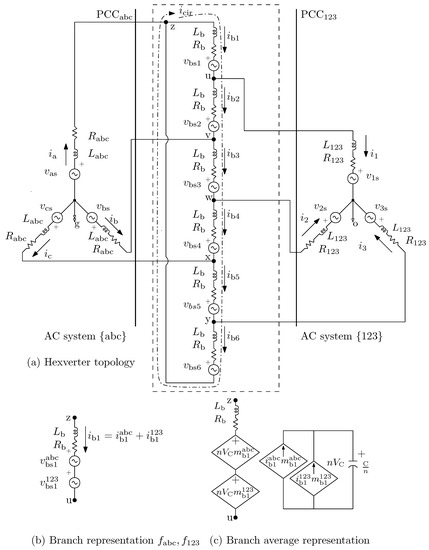
Figure 1. AC–AC Hexverter topology.

As depicted in Figure 1, the AC phase voltages of Hexverter are not referenced to ground, and the phase voltages of system $\left\{\mathrm{abc}\right\}$ are referenced to phase voltages of system $\left\{123\right\}$, and vice versa. In addition, a voltage difference $v_{\mathrm{og}}$ between both star–point potentials is set. In one hand, considering positive sequence for the supply and load of balanced AC three–phase systems, respectively, single phase voltages $\left\{\mathrm{a}\right\}$ and $\left\{1\right\}$ are fully described by (2)–(4):

$$\begin{array}{cc}\hfill v_{\mathrm{a}}& ={\widehat{v}}_{\mathrm{abc}}\cos \left({\omega }_{\mathrm{abc}}t\right),\hfill \end{array}$$

(2)

$$\begin{array}{cc}\hfill {\widehat{v}}_{123}& =p{\widehat{v}}_{\mathrm{abc}},\hfill \end{array}$$

(3)

$$\begin{array}{cc}\hfill v_1& ={\widehat{v}}_{123}\cos ({\omega }_{123}t+{\theta }_{v_{123-\mathrm{abc}}}).\hfill \end{array}$$

(4)

Voltages of system $\left\{123\right\}$ have a phase difference of ${\theta }_{v_{123-\mathrm{abc}}}$ at $t=0$ to system $\left\{\mathrm{abc}\right\}$ and p times its voltage magnitude. In the other hand, sinusoidal currents of phases $\left\{\mathrm{a}\right\}$ and $\left\{1\right\}$ are characterized by (5) and (6):

$$\begin{array}{cc}\hfill i_{\mathrm{a}}& ={\widehat{i}}_{\mathrm{abc}}\cos ({\omega }_{\mathrm{abc}}t-{\theta }_{i_{\mathrm{abc}}}),\hfill \end{array}$$

(5)

$$\begin{array}{cc}\hfill i_1& ={\widehat{i}}_{123}\cos ({\omega }_{123}t-{\theta }_{i_{123}}+{\theta }_{v_{123-\mathrm{abc}}}).\hfill \end{array}$$

(6)

Taking into account Equations (1)–(6), voltages and currents of branch ($m\in \{1,2,\dots ,6\}$) are characterized by (7) and (8):

$$\begin{array}{cc}\hfill v_{\mathrm{bs}m}& ={\widehat{v}}_{\mathrm{abc}}\cos \left({\omega }_{\mathrm{abc}}t-{\displaystyle \frac{m+1+2{(-1)}^m}{3}}\pi \right)\hfill \\ \hfill & +{\widehat{v}}_{123}\cos \left({\omega }_{123}t+{\theta }_{v_{123-\mathrm{abc}}}-{\displaystyle \frac{m-2{(-1)}^m}{3}}\pi \right)\hfill \\ \hfill & -v_{\mathrm{og}}{(-1)}^m,\hfill \end{array}$$

(7)

$$\begin{array}{cc}\hfill i_{\mathrm{b}m}& =\frac{{\widehat{i}}_{\mathrm{abc}}}{\sqrt{3}}\cos \left({\omega }_{\mathrm{abc}}t-{\theta }_{i_{\mathrm{abc}}}-{\displaystyle \frac{2m+2-{(-1)}^m}{6}}\pi \right)\hfill \\ \hfill & +\frac{{\widehat{i}}_{123}}{\sqrt{3}}\cos \left({\omega }_{123}t-{\theta }_{i_{123}}+{\theta }_{v_{123-\mathrm{abc}}}-\frac{2m+{(-1)}^m}{6}\pi \right)\hfill \\ \hfill & +i_{\mathrm{cir}}.\hfill \end{array}$$

(8)

3. Modeling and Control Approach in a Unified Two–Frequency $\mathit{d}\mathit{q}$ Framework

Recalling that by controlling the six branch voltages, $i_{\mathrm{cir}}$ can be adjusted either (i) into dynamic operation to accomplish a given energy adjustment in all branches or (ii) into steady state operation by minimizing $i_{\mathrm{cir}}$ to a minimum value [4]. Reference [3] reported that branch power transfer between adjacent branches ${\mathrm{P}}_{\mathrm{adj}}$ is function of the difference between reactive power of both AC three–phase systems. Two options to deal with this issue are listed below:

• (i) Using the “adjacent power” adjustment approach (9):

  $$\begin{array}{cc}\hfill {\mathrm{P}}_{\mathrm{adj}}& =I_{\mathrm{cir}}{V}_{\mathrm{og}},\hfill \\ \hfill {\mathrm{P}}_{\mathrm{adj}}& =\frac{\sqrt{3}}{18}\left({\mathrm{Q}}_{\mathrm{abc}}-{\mathrm{Q}}_{123}\right)\mathrm{or};\hfill \end{array}$$

  (9)
• (ii) Adjusting both reactive powers to the exact same value.

In this manuscript, both reactive power references are set equal to zero and the Hexverter–based system is operating in steady state.

3.1. Hexverter Frequency Components {$\mathrm{abc}$}

From the circuit depicted in Figure 1, considering the superposition principle, only frequency components of the AC three–phase system {$\mathrm{abc}$} are evaluated.

3.1.1. State–Space Equations {$\mathrm{abc}$} Side

Performing some mathematical derivations, the next two differential equations are obtained:

$$\begin{array}{cc}\hfill L_{\mathrm{b}}\frac{d}{dt}{i}_{\mathrm{b}135}^{\mathrm{abc}}& =v_{\mathrm{abc}}-R_{\mathrm{b}}{i}_{\mathrm{b}135}^{\mathrm{abc}}-n{V}_{\mathrm{C}}{m}_{\mathrm{b}135}^{\mathrm{abc}},\hfill \\ \hfill L_{\mathrm{b}}\frac{d}{dt}{i}_{\mathrm{b}246}^{\mathrm{abc}}& =-v_{\mathrm{bca}}-R_{\mathrm{b}}{i}_{\mathrm{b}246}^{\mathrm{abc}}-n{V}_{\mathrm{C}}{m}_{\mathrm{b}246}^{\mathrm{abc}}.\hfill \end{array}$$

(10)

Moreover, definition of the well–known cosine–based Park transformation matrix ${\mathbf{T}}_{\mathrm{xyz}}^{dq}$ is as follows:

$$\begin{array}{cc}\hfill {\mathbf{T}}_{\mathrm{xyz}}^{dq}& =\frac{2}{3}\left[\begin{array}{c}\begin{array}{ccc}\cos \left({\omega }_{\mathrm{xyz}}\right)\hfill & \cos ({\omega }_{\mathrm{xyz}}-\frac{2\pi }{3})\hfill & \cos ({\omega }_{\mathrm{xyz}}+\frac{2\pi }{3})\hfill \\ -\sin \left({\omega }_{\mathrm{xyz}}\right)\hfill & -\sin ({\omega }_{\mathrm{xyz}}-\frac{2\pi }{3})\hfill & -\sin ({\omega }_{\mathrm{xyz}}+\frac{2\pi }{3})\hfill \end{array}\end{array}\right].\hfill \end{array}$$

(11)

3.1.2. From Frequency Components {$\mathrm{abc}$} to $dq$ Transformation

Making use of ${\mathbf{T}}_{\mathrm{abc}}^{dq}$ and applying it to $i_{\mathrm{b}135}^{\mathrm{abc},dq}$ yields (12):

$$\begin{array}{cc}\hfill L_{\mathrm{b}}\frac{d}{dt}{i}_{\mathrm{b}135}^{\mathrm{abc}}& =-R_{\mathrm{b}}{i}_{\mathrm{b}135}^{\mathrm{abc}}-n{V}_{\mathrm{C}}{m}_{\mathrm{b}135}^{\mathrm{abc}}+v_{\mathrm{abc}},\hfill \\ \hfill L_{\mathrm{b}}{\mathbf{T}}_{\mathrm{abc}}^{dq}\frac{d}{dt}{i}_{\mathrm{b}135}^{\mathrm{abc}}& =-R_{\mathrm{b}}{\mathbf{T}}_{\mathrm{abc}}^{dq}{i}_{\mathrm{b}135}^{\mathrm{abc}}-n{V}_{\mathrm{C}}{\mathbf{T}}_{\mathrm{abc}}^{dq}{m}_{\mathrm{b}135}^{\mathrm{abc}}+{\mathbf{T}}_{\mathrm{abc}}^{dq}{v}_{\mathrm{abc}},\hfill \\ \hfill \frac{d}{dt}\left[\begin{array}{c}\begin{array}{c}\hfill i_{\mathrm{b}135}^{\mathrm{abc},d}\\ \hfill i_{\mathrm{b}135}^{\mathrm{abc},q}\end{array}\end{array}\right]& =\left[\begin{array}{c}\begin{array}{cc}\hfill -\frac{R_{\mathrm{b}}}{L_{\mathrm{b}}}& \hfill {\omega }_{\mathrm{abc}}\\ \hfill -{\omega }_{\mathrm{abc}}& \hfill -\frac{R_{\mathrm{b}}}{L_{\mathrm{b}}}\end{array}\end{array}\right]\left[\begin{array}{c}\begin{array}{c}\hfill i_{\mathrm{b}135}^{\mathrm{abc},d}\\ \hfill i_{\mathrm{b}135}^{\mathrm{abc},q}\end{array}\end{array}\right]-\frac{n{V}_{\mathrm{C}}}{L_{\mathrm{b}}}\left[\begin{array}{c}\begin{array}{c}\hfill m_{\mathrm{b}135}^{\mathrm{abc},d}\\ \hfill m_{\mathrm{b}135}^{\mathrm{abc},q}\end{array}\end{array}\right]+\frac{1}{L_{\mathrm{b}}}\left[\begin{array}{c}\begin{array}{c}\hfill v_{\mathrm{abc}}^d\\ \hfill v_{\mathrm{abc}}^q\end{array}\end{array}\right].\hfill \end{array}$$

(12)

Following similar steps, $i_{\mathrm{b}246}^{\mathrm{abc},dq}$ is determined by (13):

$$\begin{array}{cc}\hfill \frac{d}{dt}\left[\begin{array}{c}\begin{array}{c}\hfill i_{\mathrm{b}246}^{\mathrm{abc},d}\\ \hfill i_{\mathrm{b}246}^{\mathrm{abc},q}\end{array}\end{array}\right]& =\left[\begin{array}{c}\begin{array}{cc}\hfill -\frac{R_{\mathrm{b}}}{L_{\mathrm{b}}}& \hfill {\omega }_{\mathrm{abc}}\\ \hfill -{\omega }_{\mathrm{abc}}& \hfill -\frac{R_{\mathrm{b}}}{L_{\mathrm{b}}}\end{array}\end{array}\right]\left[\begin{array}{c}\begin{array}{c}\hfill i_{\mathrm{b}246}^{\mathrm{abc},d}\\ \hfill i_{\mathrm{b}246}^{\mathrm{abc},q}\end{array}\end{array}\right]-\frac{n{V}_{\mathrm{C}}}{L_{\mathrm{b}}}\left[\begin{array}{c}\begin{array}{c}\hfill m_{\mathrm{b}246}^{\mathrm{abc},d}\\ \hfill m_{\mathrm{b}246}^{\mathrm{abc},q}\end{array}\end{array}\right]-\frac{1}{L_{\mathrm{b}}}\left[\begin{array}{c}\begin{array}{c}\hfill v_{\mathrm{bca}}^d\\ \hfill v_{\mathrm{bca}}^q\end{array}\end{array}\right].\hfill \end{array}$$

(13)

3.2. Hexverter Frequency Components {123}

In this case, only frequency components of AC three–phase system {123} are considered.

3.2.1. State–Space Equations {123} Side

Next, by performing some mathematical manipulations, two differential equations are derived:

$$\begin{array}{cc}\hfill L_{\mathrm{b}}\frac{d}{dt}{i}_{\mathrm{b}135}^{123}& =-v_{123}-R_{\mathrm{b}}{i}_{\mathrm{b}135}^{123}-n{V}_{\mathrm{C}}{m}_{\mathrm{b}135}^{123},\hfill \\ \hfill L_{\mathrm{b}}\frac{d}{dt}{i}_{\mathrm{b}246}^{123}& =v_{123}-R_{\mathrm{b}}{i}_{\mathrm{b}246}^{123}-n{V}_{\mathrm{C}}{m}_{\mathrm{b}246}^{123}.\hfill \end{array}$$

(14)

3.2.2. From Frequency Components {123} to $dq$ Transformation

Using the ${\mathbf{T}}_{123}^{dq}$ transformation matrix, $i_{\mathrm{b}135}^{123,dq}$ is derived as in (15):

$$\begin{array}{cc}\hfill \frac{d}{dt}\left[\begin{array}{c}\begin{array}{c}\hfill i_{\mathrm{b}135}^{123,d}\\ \hfill i_{\mathrm{b}135}^{123,q}\end{array}\end{array}\right]& =\left[\begin{array}{c}\begin{array}{cc}\hfill -\frac{R_{\mathrm{b}}}{L_{\mathrm{b}}}& \hfill {\omega }_{123}\\ \hfill -{\omega }_{123}& \hfill -\frac{R_{\mathrm{b}}}{L_{\mathrm{b}}}\end{array}\end{array}\right]\left[\begin{array}{c}\begin{array}{c}\hfill i_{\mathrm{b}135}^{123,d}\\ \hfill i_{\mathrm{b}135}^{123,q}\end{array}\end{array}\right]-\frac{n{V}_{\mathrm{C}}}{L_{\mathrm{b}}}\left[\begin{array}{c}\begin{array}{c}\hfill m_{\mathrm{b}135}^{123,d}\\ \hfill m_{\mathrm{b}135}^{123,q}\end{array}\end{array}\right]-\frac{1}{L_{\mathrm{b}}}\left[\begin{array}{c}\begin{array}{c}\hfill v_{123}^d\\ \hfill v_{123}^q\end{array}\end{array}\right].\hfill \end{array}$$

(15)

Correspondingly, $i_{\mathrm{b}246}^{123,dq}$ is determined by (16):

$$\begin{array}{cc}\hfill \frac{d}{dt}\left[\begin{array}{c}\begin{array}{c}\hfill i_{\mathrm{b}246}^{123,d}\\ \hfill i_{\mathrm{b}246}^{123,q}\end{array}\end{array}\right]& =\left[\begin{array}{c}\begin{array}{cc}\hfill -\frac{R_{\mathrm{b}}}{L_{\mathrm{b}}}& \hfill {\omega }_{123}\\ \hfill -{\omega }_{123}& \hfill -\frac{R_{\mathrm{b}}}{L_{\mathrm{b}}}\end{array}\end{array}\right]\left[\begin{array}{c}\begin{array}{c}\hfill i_{\mathrm{b}246}^{123,d}\\ \hfill i_{\mathrm{b}246}^{123,q}\end{array}\end{array}\right]-\frac{n{V}_{\mathrm{C}}}{L_{\mathrm{b}}}\left[\begin{array}{c}\begin{array}{c}\hfill m_{\mathrm{b}246}^{123,d}\\ \hfill m_{\mathrm{b}246}^{123,q}\end{array}\end{array}\right]+\frac{1}{L_{\mathrm{b}}}\left[\begin{array}{c}\begin{array}{c}\hfill v_{123}^d\\ \hfill v_{123}^q\end{array}\end{array}\right].\hfill \end{array}$$

(16)

3.3. Control Approach

From (12), the next differential equations are obtained:

$$\begin{array}{cc}\hfill \frac{d}{dt}{i}_{\mathrm{b}135}^{\mathrm{abc},d}& =-\frac{R_{\mathrm{b}}}{L_{\mathrm{b}}}{i}_{\mathrm{b}135}^{\mathrm{abc},d}+{\omega }_{\mathrm{abc}}{i}_{\mathrm{b}135}^{\mathrm{abc},q}-\frac{n{V}_{\mathrm{C}}}{L_{\mathrm{b}}}{m}_{\mathrm{b}135}^{\mathrm{abc},d}+\frac{1}{L_{\mathrm{b}}}{v}_{\mathrm{abc}}^d,\hfill \end{array}$$

(17)

$$\begin{array}{cc}\hfill \frac{d}{dt}{i}_{\mathrm{b}135}^{\mathrm{abc},q}& =-{\omega }_{\mathrm{abc}}{i}_{\mathrm{b}135}^{\mathrm{abc},d}-\frac{R_{\mathrm{b}}}{L_{\mathrm{b}}}{i}_{\mathrm{b}135}^{\mathrm{abc},q}-\frac{n{V}_{\mathrm{C}}}{L_{\mathrm{b}}}{m}_{\mathrm{b}135}^{\mathrm{abc},q}+\frac{1}{L_{\mathrm{b}}}{v}_{\mathrm{abc}}^q,\hfill \end{array}$$

(18)

making use of a change of variable as follows:

$$\begin{array}{cc}\hfill m_{\mathrm{b}135}^{\mathrm{abc},d}& =\frac{1}{n{V}_{\mathrm{C}}}\left(-u_{135}^{\mathrm{abc},d}+L_{\mathrm{b}}{\omega }_{\mathrm{abc}}{i}_{\mathrm{b}135}^{\mathrm{abc},q}+v_{\mathrm{abc}}^d\right),\hfill \end{array}$$

(19)

$$\begin{array}{cc}\hfill m_{\mathrm{b}135}^{\mathrm{abc},q}& =\frac{1}{n{V}_{\mathrm{C}}}\left(-u_{135}^{\mathrm{abc},q}-L_{\mathrm{b}}{\omega }_{\mathrm{abc}}{i}_{\mathrm{b}135}^{\mathrm{abc},d}+v_{\mathrm{abc}}^q\right),\hfill \end{array}$$

(20)

two independent and decoupled equations are obtained, which stand for $dq$ components of branch currents {135} at frequency {abc}; those are described by (21):

$$\begin{array}{cc}\hfill \frac{d}{dt}{i}_{\mathrm{b}135}^{\mathrm{abc},d}& =-\frac{R_{\mathrm{b}}}{L_{\mathrm{b}}}{i}_{\mathrm{b}135}^{\mathrm{abc},d}+\frac{1}{L_{\mathrm{b}}}{u}_{135}^{\mathrm{abc},d},\hfill \\ \hfill \frac{d}{dt}{i}_{\mathrm{b}135}^{\mathrm{abc},q}& =-\frac{R_{\mathrm{b}}}{L_{\mathrm{b}}}{i}_{\mathrm{b}135}^{\mathrm{abc},q}+\frac{1}{L_{\mathrm{b}}}{u}_{135}^{\mathrm{abc},q}.\hfill \end{array}$$

(21)

Similar mathematical manipulations can be conducted with Equations (13), (15), and (16) in order to obtain decoupled equations to control branch currents {$i_{\mathrm{b}246}^{\mathrm{abc},d}$}, {$i_{\mathrm{b}246}^{\mathrm{abc},q}$}, {$i_{\mathrm{b}135}^{123,d}$}, {$i_{\mathrm{b}135}^{123,q}$}, {$i_{\mathrm{b}246}^{123,d}$}, and {$i_{\mathrm{b}246}^{123,q}$}. This set of equations is an equivalent and decoupled representation of the former set of differential equations that can be managed and transformed into the Laplace domain. Afterwards, by applying techniques from [16], a suitable control scheme in a unified two–frequency $dq$ framework for a Hexverter–based system is elaborated.

3.4. Branch Current Controllers

Variable $\mathbf{x}={[i_{\mathrm{b}135}^{\mathrm{abc},dq},i_{\mathrm{b}246}^{\mathrm{abc},dq},i_{\mathrm{b}135}^{123,dq},i_{\mathrm{b}246}^{123,dq}]}^{\prime }$ corresponds to a column vector that includes the state variables. From this, $i_{\mathrm{b}135}^{\mathrm{abc},dq}$ indicates $dq$ components of currents flowing through branches {135} at frequency {abc}. The same notation applies for the rest of the state variables. Each branch current controller outputs a three–phase modulating signal labeled as $m_{\mathrm{b}135}^{\mathrm{abc}}$, $m_{\mathrm{b}246}^{\mathrm{abc}}$, $m_{\mathrm{b}135}^{123}$, and $m_{\mathrm{b}246}^{123}$. These signals are then de–multiplexed and recombined as follows: $m_{\mathrm{b}1}=m_{\mathrm{b}1}^{\mathrm{abc}}+m_{\mathrm{b}1}^{123}, m_{\mathrm{b}2}=m_{\mathrm{b}2}^{\mathrm{abc}}+m_{\mathrm{b}2}^{123}, \dots , m_{\mathrm{b}6}=m_{\mathrm{b}6}^{\mathrm{abc}}+m_{\mathrm{b}6}^{123}$. Afterwards, these signals are augmented by the reference branch voltage $n{V}_{\mathrm{C}}^{*}$, generating reference branch voltages $v_{\mathrm{bs}m}^{*}$, which are suitable inputs for the modulator. A general schematic of a single branch current controller is depicted in Figure 2. From it, {$\mathrm{xyz}$} stands for frequency {$\mathrm{abc}$} or {123}, respectively. Figure 2 shows two main subsystems marked as “power–to–current” and “branch current control”. As depicted, the branch current’s error is driven to zero through a decoupled PI compensator. For instance, if {$\mathrm{xyz}$} is replaced by {$\mathrm{abc}$}, then the schematic agrees with the state variable [$i_{\mathrm{b}135}^{\mathrm{abc},dq}$], and as a consequence, the modulation index $m_{\mathrm{b}135}^{\mathrm{abc}}$ is the output of the subsystem “branch current control”. Analogous diagrams of branch current controllers corresponding to state variables $i_{\mathrm{b}246}^{\mathrm{abc},dq}$, $i_{\mathrm{b}135}^{123,dq}$, and $i_{\mathrm{b}246}^{123,dq}$ can be elaborated [17].

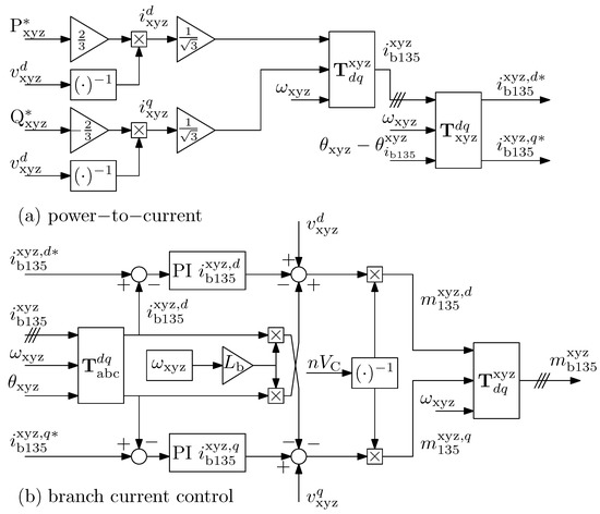
Figure 2. Block diagrams of current control to determine $m_{\mathrm{b}135}^{\mathrm{xyz}}$.

4. Modulation Strategies

This section is devoted to describe in depth two modulation techniques that will further be assessed when implemented into the Hexverter–based system.

4.1. Nearest Level Control

Some of the features that make NLC an attractive option to modulate a modular multilevel converter are its (i) comparatively low switching frequency, (ii) it is simple to implement, and (iii) it is remarkably suitable for a power converter that require a large number of levels [18,19,20]. Notice the objective of NLC is to determine “how many” SMs per branch $n_m$ are going to be connected/bypassed at any given time. A detailed diagram depicting the implementation of NLC is shown in Figure 3. First, branch reference voltage $v_{\mathrm{bs}m}^{*}$, containing two frequency components ($f_{\mathrm{abc}},f_{123}$), is the input. Right after, it is divided by a SM reference voltage $V_{\mathrm{C}}^{*}$ and rounded. Then, variable $n_m$ indicating the number of SMs to be inserted/bypass for each branch m is obtained. In the end, in regard to positive or negative values of $n_m$, variables $n_{\mathrm{up}m}$ and $n_{\mathrm{down}m}$ are calculated.

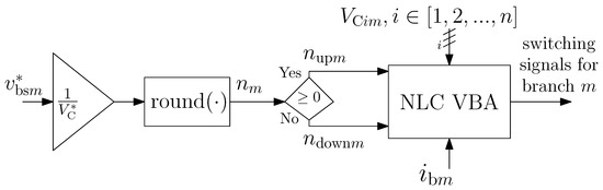
Figure 3. General flowchart of NLC modulation technique.

Recalling, each full–bridge submodule contains a capacitor that is set to a reference voltage denoted as $V_{\mathrm{C}}^{*}$. Since each submodule will switch to synthesize AC voltage on its terminals, voltage variations of $V_{\mathrm{C}}$ will occur. Therefore, with the objective to minimize $V_{\mathrm{C}}$ fluctuations of each submodule, a voltage–balancing algorithm (VBA) utilized by NLC is shown in Figure 4. The sorting process is performed by the use of the merge–sort algorithm, which is an efficient, general–purpose and comparison–based sorting algorithm. It was proposed in 1945 by John von Neumann [21]. As illustrated, the inputs are (i) the number of SMs $n_{\mathrm{up}m}$, (ii) measurements of capacitors’ voltage comprising each branch $V_{\mathrm{C}im}$, and (iii) measurements of currents flowing through each branch $i_{\mathrm{b}m}$. Thus, “which” of the submodules required to be inserted/bypassed for each Hexverter branch when synthesizing positive semi–cycles can be determined.

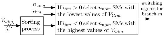
Figure 4. NLC VBA flowchart.

When variable $n_{\mathrm{up}m}$ is substituted by $n_{\mathrm{down}m}$ in Figure 4,“which” of the SMs required to be connected/bypassed for each Hexverter branch are known. The performance evaluation of NLC VBA is discussed in Section 7.1.

4.2. Phase Disposition–Sinusoidal Pulse Width Modulation

PD–SPWM is an extended version of the standard pulse width modulation strategy. In this case, n number of triangular waveforms [$v_k$ = carriers] are employed, shown in Figure 5. Each carrier has an amplitude of $|v_k|=-1+\frac{2k-1}{n}$, where $k\in \{1,2,\dots ,n\}$. As it can be seen, each carrier features a symmetrical offset with respect to the horizontal zero–axis. These carriers, when compared to a provided sinusoidal reference $\pm v_{\mathrm{bs}m}^{*}$, are employed to specifically compute the number of series connected H–bridge SMs to be connected/bypassed at any given time. Variable $n_{\mathrm{up}m}$ stores values when $+v_{\mathrm{bs}m}^{*}$ is used, whereas variable $n_{\mathrm{down}m}$ stores values when $-v_{\mathrm{bs}m}^{*}$ is utilized. A flowchart describing the process to determine $n_{\mathrm{up}m}$ is shown in Figure 6.

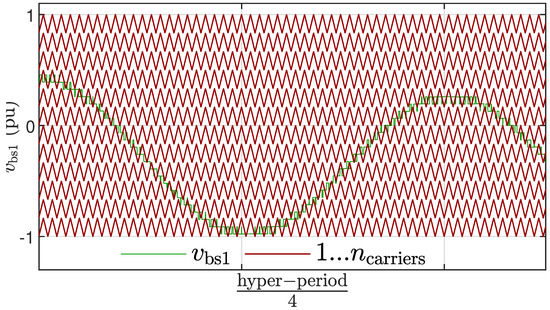
Figure 5. Twelfth PD–SPWM carriers and synthesized voltage.

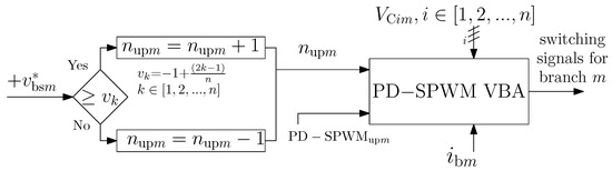
Figure 6. General flowchart of PD–SPWM modulation technique.

The next step is to determine “which” of the SMs will be connected at any given time; to this end, a PD–SPWM VBA is implemented. It is depicted in Figure 7. The sorting process is performed by the use of the merge–sort algorithm. As shown, the inputs are (i) the number of SMs $n_{\mathrm{up}m}$, (ii) the measurements of capacitors’ voltage of each branch $V_{\mathrm{C}im}$, (iii) the measurements of currents flowing through each branch $i_{\mathrm{b}m}$, and (iv) the trigger signals of each branch $\mathrm{PD}-{\mathrm{SPWM}}_{\mathrm{up}m}$. The internal process of the PD–SPWM VBA is illustrated in Figure 7, where the output is a set of switching signals for each SM comprising any of the Hexverter’ branches.

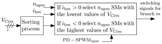
Figure 7. PD–SPWM VBA flowchart.

If variable $+v_{\mathrm{bs}m}^{*}$ is replaced by $-v_{\mathrm{bs}m}^{*}$ in Figure 6, variable $n_{\mathrm{down}m}$ and trigger signals $\mathrm{PD}-{\mathrm{SPWM}}_{\mathrm{down}m}$ are calculated. Additionally, by plugging those in Figure 7, instead of $n_{\mathrm{up}m}$ and $\mathrm{PD}-{\mathrm{SPWM}}_{\mathrm{up}m}$, switching signals for each submodule forming a Hexverter branch m are obtained. The performance assessment of PD–SPWM VBA is presented in Section 7.2.

Each carrier features a switching frequency of $f_{\mathrm{sw}}$ = 5 kHz. However, on average, each SM will switch at $\frac{f_{\mathrm{sw}}}{n}$ = 334 Hz per hyper–period. Be aware that a hyper–period is defined as ${\mathrm{T}}_h$ = 1/$\gcd (f_{\mathrm{abc}},f_{123})$.

5. Proposed “Virtual ${\mathit{V}}_{\mathbf{C}}^{\mathbf{2}}$ Controller”

In order for the Hexverter–based system to perform properly, active and reactive power references ($P_{\mathrm{abc}}^{*}$, $Q_{\mathrm{abc}}^{*}$, $P_{123}^{*}$, and $Q_{123}^{*}$) must be provided. However, as depicted in Figure 10, active power reference $P_{123}^{*}$ is dependent of the Hexverter’s active power losses ($\Delta P$). In general, $\Delta P$ is composed of (i) energy variations in the elements storing energy ($P_{\mathrm{C}}$ and $P_{\mathrm{L}}$), (ii) active power losses due to the switching ($P_{\mathrm{sw}}$) and conduction ($P_{\mathrm{cond}}$) of semiconductors, and (iii) active power losses due to parasitic effects of the Hexverter’ elements which are typically modeled as resistors dissipating power ($P_{\mathrm{R}}$). In this research, an approach to determine active power losses “$\Delta P$” is studied and proposed. The main objectives are (i) to achieve active power balance on the fly of the Hexverter–based system and (ii) to keep the submodules’ capacitor voltage as close as possible to the given reference, so that almost all the incoming power can be transferred into the load. As shown earlier in this document, the Hexverter topology does not feature a real DC link between the connection of two AC three–phase systems; however, a “virtual DC link” can be modeled by calculating an average DC voltage per submodule of each Hexverter’ branch. The DC voltage provided as the reference $V_{\mathrm{C}}^{*}$, which in turn is the initial voltage over each full–bridge submodule before starting the operation of the Hexverter system, can be calculated as follows:

$$\begin{array}{c}\hfill V_{\mathrm{C}}^{*}=\frac{{\widehat{v}}_{\mathrm{abc}}+{\widehat{v}}_{123}}{n}.\end{array}$$

(22)

Considering only elements storing energy inside the Hexverter system and ideal behavior of the power converter ($P_{\mathrm{sw}}=0$ ) and ($P_{\mathrm{cond}}=0$), a general figure of the Hexverter system is shown in Figure 8. By the use of Poynting’s theorem, Equation (23) is derived:

$$\begin{array}{c}\hfill P_{\mathrm{abc}}=\underset{\Delta P}{\underbrace{\sum _{m=1}^6\sum _{i=1}^n\frac{d}{dt}\frac{1}{2}C{V}_{{\mathrm{C}}_{im}}^2+\sum _{i=1}^m\frac{d}{dt}\frac{1}{2}{L}_{\mathrm{b}}{i}_{\mathrm{b}m}^2+(P_{\mathrm{sw}}=0)+(P_{\mathrm{cond}}=0)+P_{\mathrm{R}}}}+P_{123}.\end{array}$$

(23)

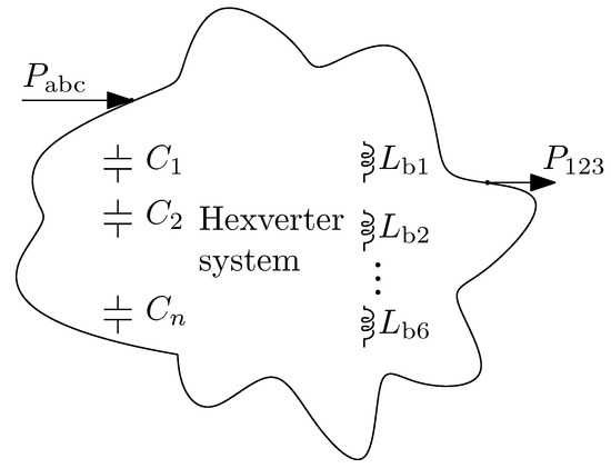
Figure 8. Elements storing energy in the Hexverter system.

Since the energy stored over the branch inductors is relatively low in comparison to the energy stored in the capacitors of each submodule, and the active power dissipated by the $P_{\mathrm{R}}$ term will add a DC offset, the active power losses “$\Delta P$” can be estimated by considering the rate of change in the energy stored in the capacitors only. In other words, Equation (23) becomes:

$$\begin{array}{c}\hfill P_{\mathrm{abc}}=\underset{\Delta P}{\underbrace{\sum _{m=1}^6\sum _{i=1}^n\frac{d}{dt}\frac{1}{2}C{V}_{{\mathrm{C}}_{im}}^2}}+P_{123}.\end{array}$$

(24)

Specifically, an approximation to determine “$\Delta P$” is described by:

$$\begin{array}{cc}\hfill \Delta P& =\frac{1}{2}C\sum _{m=1}^6\sum _{i=1}^n\frac{d}{dt}{V}_{{\mathrm{C}}_{im}}^2.\hfill \end{array}$$

(25)

In this work, this fact is used in order to compute the Hexverter’s active power losses “$\Delta P$”. Furthermore, this will achieve an active power balance of the Hexverter–based system on the fly. A general scheme of the so–called “virtual $V_{\mathrm{C}}^2$ controller” is shown in Figure 9.

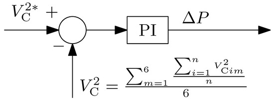
Figure 9. Virtual $V_{\mathrm{C}}^2$ controller block diagram.

To validate the performance of the proposed “Virtual $V_{\mathrm{C}}^2$ controller” under different scenarios, Test Case I and Test Case II are developed. In Test Case I, the Hexverter–based system is considered to function keeping ideal behavior, in the sense that $P_{\mathrm{sw}}$ and $P_{\mathrm{cond}}$ are both equal to zero. By contrast, in Test Case II, a more realistic scenario of the Hexverter–based system is assessed when $P_{\mathrm{sw}}^{\mathrm{T}}$ and $P_{\mathrm{cond}}^{\mathrm{T}}$ of the IGBT’s and $P_{\mathrm{cond}}^{\mathrm{D}}$ of diodes are taken into account. As described earlier, the calculation of $\Delta P$ is a necessary condition to compute the active power ($P_{123}^{*}$) reference value for the {123} side. Once $P_{123}^{*}$ and $Q_{123}^{*}$ are entered into the “power–to–current” subsystem depicted in Figure 2a, the correct reference values for branch currents $i_{\mathrm{b}135}^{123,dq*}$ and $i_{\mathrm{b}246}^{123,dq*}$ are obtained.

6. Hexverter–Based System Integration

A general schematic of the Hexverter–based system is portrayed in Figure 10. It shows the integration of the subsystems’ “virtual $V_{\mathrm{C}}^2$ controller” Figure 9; the branch current controllers in a unified $dq$ framework in Figure 2a,b; modulator Figure 3; voltage balancing algorithm Figure 4l and the Hexverter system shown above in Figure 1. Initially, the active and reactive power references of the {abc} side ($P_{\mathrm{abc}}^{*}$ and $Q_{\mathrm{abc}}^{*}$) are necessary operational inputs to the “power–to–current” subsystem depicted in Figure 2a, which, in turn, output reference values of branch currents $i_{\mathrm{b}135}^{\mathrm{abc},dq*}$ and $i_{\mathrm{b}246}^{\mathrm{abc},dq*}$, respectively. Then, $\Delta P$ obtained from the “virtual $V_{\mathrm{C}}^2$ controller” is subtracted to $P_{\mathrm{abc}}^{*}$ to determine active power reference $P_{123}^{*}$. Based on operational conditions reactive power reference ($Q_{123}^{*}$) is set. These power references are fed into the “power–to–current” subsystem depicted in Figure 2a, outputting reference values of branch currents $i_{\mathrm{b}135}^{123,dq*}$ and $i_{\mathrm{b}246}^{123,dq*}$, respectively. Once ${\mathrm{x}}^{*}$ is complete, it is compared against proper measurements, and its error is fed into the branch current controller shown in Figure 2b. Modulation indices $m_{\mathrm{b}m}$, which are outputs of the branch current controllers, become inputs for a modulator, either NLC or PD–SPWM, see Figure 3 or Figure 6. According to the selected modulation strategy, the modulator outputs the number of submodules to be connected ($n_m$) at any given time. This is the input for the VBA that in turn generates switching signals for each power submodule comprising each Hexverter branch.

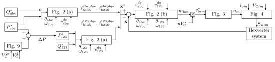
Figure 10. Hexverter-based system integration.

7. Simulation Results

Detailed simulations are implemented into the software platform PSCAD/EMTDC [22]. The objective is to verify the operation and performance of the Hexverter power converter under the application of modulations techniques NLC and PD–SPWM. The reader is referred to Table 1, where simulation parameters are listed. Meanwhile, an experimental prototype is being built in the author’s laboratory.

Table 1. Simulation parameters.

	Branch resistance	$R_b$	0.6 $\mathsf{\Omega }$
	Branch inductance	$L_{\mathrm{b}}$	10 mH
Hexverter	Number of SMs per branch	n	12
	Capacitance	C	20 mF
	Nominal SM voltage	$V_{\mathrm{C}}$	166.67 V
	Active power	${\mathrm{P}}_{\mathrm{abc}}$	15 kVA
	Reactive power	${\mathrm{Q}}_{\mathrm{abc}}$	0 kVar
	Voltage magnitude	$v_{\mathrm{abc}}$	1 kV
System {abc}	Frequency	$f_{\mathrm{abc}}$	50 Hz
	Resistance	$R_{\mathrm{abc}}$	1 $\mathsf{\Omega }$
	Inductance	$L_{\mathrm{abc}}$	10 mH
	Active power	${\mathrm{P}}_{123}$	from $V_{\mathrm{C}}^2$ control
	Reactive power	${\mathrm{Q}}_{123}$	0 kVar
	Voltage magnitude	$v_{123}$	1 kV
System {123}	Frequency	$f_{123}$	10 Hz
	Resistance	$R_{123}$	0.8 $\mathsf{\Omega }$
	Inductance	$L_{123}$	15 mH
	Voltage between neutrals	$v_{\mathrm{og}}$	0 V
	Circulating current	$i_{\mathrm{cir}}$	0 A

7.1. NLC Simulation Results

Recalling that both three–phase systems are labeled as {abc} or {123}, Figure 11 shows the top two sub–figures depicting waveforms corresponding to AC voltages $v_{\mathrm{abc}}$ and $v_{123}$. Comparing the provided simulation parameters, both AC voltages show good match in magnitude, frequency, and phase.

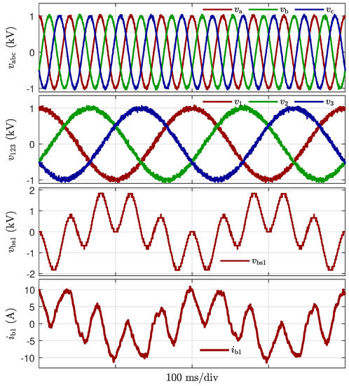
Figure 11. NLC: AC three–phase voltages $v_{\mathrm{abc}},v_{123}$, branch voltage $v_{\mathrm{bs}1}$, and branch current $i_{\mathrm{b}1}$.

In addition, at the bottom of Figure 11, two more waveforms are presented. In one hand, $v_{\mathrm{bs}1}$ corresponds to synthesized branch voltage utilizing NLC modulation technique. As observed, it features typical “discrete steps or levels”, indicating NLC has been precisely implemented. Moreover, a voltage magnitude nearly of 2 kV can be measured. On the other hand, $i_{\mathrm{b}1}$ depicts current that flows through branch one. A current magnitude close to 10 Amperes is shown. Furthermore, by carefully observing traces of voltage $v_{\mathrm{bs}1}$ and current $i_{\mathrm{b}1}$, it can be realized that they feature both frequency components ($f_{\mathrm{abc}},f_{123}$) of the connected AC three–phase systems. In summary, it can be mentioned that both $v_{\mathrm{bs}1}$ and $i_{\mathrm{b}1}$ are fully compliant to Equations (7) and (8). With regard to the performance of the so–called NLC VBA, Figure 12 illustrates n traces that correspond to measurements of controlled capacitor’s voltage. Based on the reported results, it can be stated that NLC VBA is controlling n voltages between a reasonable range of $V_{\mathrm{C}i1}=\pm 2.5\mathrm{V}$. This variation is approximately equal to 1.5% average error in comparison to $V_{\mathrm{C}}^{*}$. NLC VBA achieves a steady–state in about 200 ms.

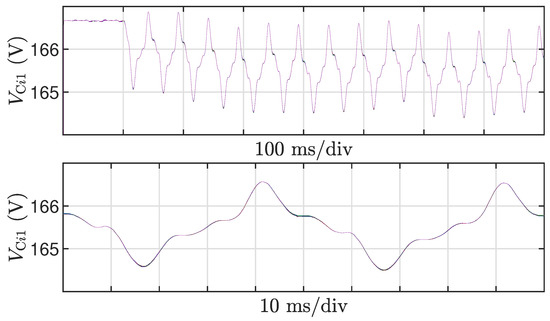
Figure 12. NLC VBA performance: (Top) zoom–out depicting transients at initial conditions; (Bottom) zoom–in at steady–state.

7.2. PD–SPWM Simulation Results

The top two sub–figures of Figure 13 depict waveforms corresponding to AC voltages $v_{\mathrm{abc}}$ and $v_{123}$, respectively. These are compliant with the provided simulation parameters due to the fact that a good match in magnitude, frequencies, and phase is observed. Moreover, the bottom two sub–figures depict waveforms of $v_{\mathrm{bs}1}$ and $i_{\mathrm{b}1}$, respectively. With respect to $v_{\mathrm{bs}1}$, it shows a peak voltage of approximately 2 kV. Its trace shows typical on and off switching over the “levels” indicating PD–SPWM has been adequately implemented into the simulation. Current flowing through branch one is shown by trace $i_{\mathrm{b}1}$. As expected, a peak value of about 10 Amperes can be measured. Consistent with Equations (7) and (8), $v_{\mathrm{bs}1}$ and $i_{\mathrm{b}1}$ contain both frequency components ($f_{\mathrm{abc}},f_{123}$) of the connected AC three-phase systems.

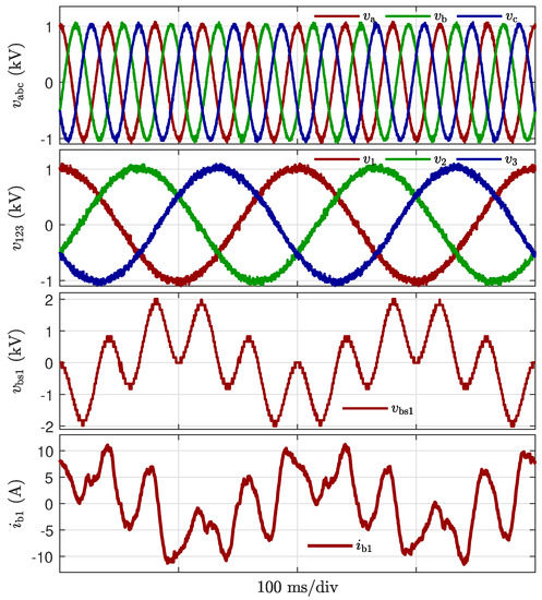
Figure 13. PD–SPWM: AC three–phase voltages $v_{\mathrm{abc}},v_{123}$, branch voltage $v_{\mathrm{bs}1}$, and branch current $i_{\mathrm{b}1}$.

Performance of PD–SPWM VBA is presented in Figure 14, where n number of controlled capacitors’ voltage waveforms are depicted. PD–SPWM VBA is controlling all branch capacitor’s voltages $V_{\mathrm{C}i1}=\pm 3.0\mathrm{V}$ compared to $V_{\mathrm{C}}^{*}$, representing a 1.80% average error. PD–SPWM VBA performs the same in all other branches. It reaches steady–state in about 300 ms.

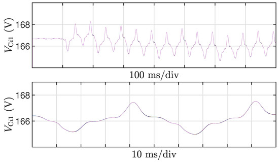
Figure 14. PD–SPWM VBA performance: (Top) zoom–out depicting transients at initial conditions; (Bottom) zoom–in at steady–state.

7.3. NLC and PD–SPWM Discussion of Results

Regarding the implementation of NLC and PD–SPWM into the Hexverter-based multilevel converter and based on simulation results shown from Figure 11, Figure 12, Figure 13 and Figure 14, three main points can be mentioned. (i) Since, with the naked eye, almost no difference can be observed in both synthesized AC voltages and currents, it becomes necessary to analyze these waveforms in depth. Thus, in order to determine which modulation technique outperform the other in terms of its harmonic spectrum and total harmonic distortion, the reader is referred to Section 9. (ii) On one hand, branch $v_{\mathrm{bs}1}$ voltages show a small difference in the number of levels to synthesize the same Hexverter’ terminal voltages; on the other hand, both branch currents $i_{\mathrm{b}1}$ are clearly different, it can be mentioned that the branch current out of PD–SPWM is more distorted than the one measured when the NLC modulation technique is utilized. (iii) A small difference of a 0.3% average error is measured when comparing both voltage balancing algorithms.

8. Performance of “Virtual ${\mathit{V}}_{\mathbf{C}}^{\mathbf{2}}$ Controller”

In order to validate the performance of the “virtual $V_{\mathrm{C}}^2$ controller” two different scenarios are considered.

8.1. Test Case I

In this scenario, the Hexverter power converter is considered a lossless system. In other words, $P_{\mathrm{sw}}$ and $P_{\mathrm{cond}}$ are both equal to zero. Be aware that the parasitic effects of the Hexverter’ reactive elements are modeled into the branch resistor $R_{\mathrm{b}}$. The performance of “virtual $V_{\mathrm{C}}^2$ control” under the NLC modulation technique is depicted in Figure 15. At the beginning of the trace, a transient behavior appears due to the rate of change in energy into the submodule’s capacitor and branch inductors; nevertheless, under these transient conditions, the controller is able to achieve and provide a correct active power balance reference for the AC system {123}. As observed, the controller takes approximately 1.25 s to reach steady–state with a $\Delta P$ value of 184 W. By analyzing Equation (23), this value of $\Delta P$ parameter corresponds to a DC offset due to the embedded calculation of the $P_{\mathrm{R}}$ term. In order to verify the correctness of the calculated $\Delta P$ value, the reader is referred to Table 1, where the active power reference of the AC system {abc} ${\mathrm{P}}_{\mathrm{abc}}^{*}=$ 15 kVA is provided.

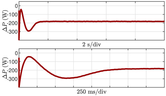
Figure 15. Test Case I: NLC $\Delta P$ value obtained with “virtual $V_{\mathrm{C}}^2$ control”.

In the same fashion, performance of “virtual $V_{\mathrm{C}}^2$ control” under PD–SPWM modulation technique is depicted in Figure 16. As expected, a transient behavior of $\Delta P$ trace appears at the beginning. However, one more time, the controller is able to achieve and provide correct active power balance reference for the AC system {123}. As it is depicted, the controller takes about 1.5 s to achieve steady state with a value of 202 W, that corresponds to a DC offset due to the embedded calculation of $P_{\mathrm{R}}$ term. By comparing both $\Delta P$ parameter values out of both modulation techniques, an active power difference of 18 W is observed. It seems that by utilizing this simulation setup, active power losses are 18 W higher when PD–SPWM is utilized.

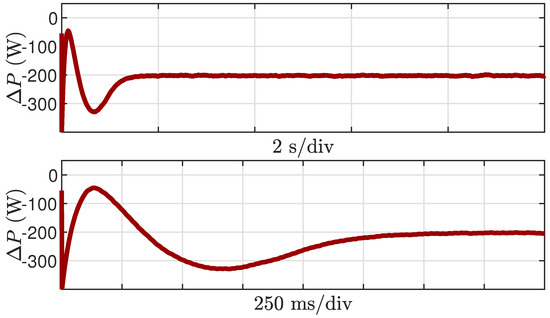
Figure 16. Test Case I: PD–SPWM $\Delta P$ parameter obtained with “virtual $V_{\mathrm{C}}^2$ control”.

8.2. Test Case II

In this scenario, the Hexverter power converter is no longer considered a lossless system. The IGBT transistor part number IRG4BC30KDPbF is selected. Its main parameters are listed in Table 2, and it includes an ultrafast soft recovery diode connected in antiparallel. Since all branch reference voltages coming out of the implemented current controllers, submodules’ DC link voltages, and branch current directions are known, the duty cycles for the IGBTs and diodes defined with variables ($d_{\mathrm{b},mi}^{\mathrm{T}}$ and $d_{\mathrm{b},mi}^{\mathrm{D}}$) can be determined [3]. Switching and conduction losses of a single transistor are defined by variables $P_{\mathrm{sw}}^{\mathrm{T}}$ and $P_{\mathrm{cond}}^{\mathrm{T}}$, respectively. These can be estimated by Equations (26) and (27), respectively:

$$\begin{array}{cc}\hfill P_{\mathrm{sw}}^{\mathrm{T}}& =(E_{{\mathrm{ON}}_{\mathrm{T}}}+E_{{\mathrm{OFF}}_{\mathrm{T}}})\frac{V_{\mathrm{Throw}}\overline{i_{\mathrm{T}}}}{V_{{\mathrm{REF}}_{\mathrm{T}}}{I}_{{\mathrm{REF}}_{\mathrm{T}}}}{f}_{\mathrm{sw}}\hfill \end{array}$$

(26)

$$\begin{array}{cc}\hfill P_{\mathrm{cond}}^{\mathrm{T}}& =d_{\mathrm{b},mi}^{\mathrm{T}}{V}_{{\mathrm{CE}}_{{\mathrm{ON}}_{\mathrm{T}}}}\overline{i_{\mathrm{T}}}.\hfill \end{array}$$

(27)

Similarly, the conduction loss of a single diode is defined by variable $P_{\mathrm{cond}}^{\mathrm{D}}$ and can be approximated by Equation (28):

$$\begin{array}{cc}\hfill P_{\mathrm{cond}}^{\mathrm{D}}& =d_{\mathrm{b},mi}^{\mathrm{D}}{V}_{{\mathrm{F}}_{\mathrm{D}}}\overline{i_{\mathrm{D}}}.\hfill \end{array}$$

(28)

Bear in mind, $\overline{i_{\mathrm{T}}}$ and $\overline{i_{\mathrm{D}}}$ are both equal to the magnitude of branch current $|i_{\mathrm{b},m}|$, and $V_{\mathrm{Throw}}$ is equal to the given reference voltage for each submodule $V_{\mathrm{C}}^{*}$. Furthermore, in order to determine the mean values for the active power losses, all calculations are performed over a hyper–period defined earlier as $T_h=1/\gcd (f_{\mathrm{abc}},f_{123})$.

Table 2. Nominal parameters of the IGBT and Diode part number: IRG4BC30KDPbF and operational conditions.

Transistor	Collector–to–emitter voltage	$V_{\mathrm{CES}}$	600 V
	Continuous collector current	$I_{\mathrm{C}}@$$T_{\mathrm{C}}$ = 25 °C	28 A
	Collector–to–emitter saturation voltage	$V_{{\mathrm{CE}}_{{\mathrm{ON}}_{\mathrm{T}}}}$	2.21 V
	Turn–on switching loss	$E_{{\mathrm{ON}}_{\mathrm{T}}}$	0.60 mJ
	Turn–off switching loss	$E_{{\mathrm{OFF}}_{\mathrm{T}}}$	0.58 mJ
Diode	Continuous forward current	$I_{{\mathrm{F}}_{\mathrm{D}}}$	12 A
	Forward voltage drop	$V_{{\mathrm{F}}_{\mathrm{D}}}$	1.4 V
Operational	Operating voltage	$V_{{\mathrm{REF}}_{\mathrm{T}}}$	167 V
conditions	Peak value of operating current	${\widehat{I}}_{{\mathrm{REF}}_{\mathrm{T}}}$	10 A
	Transistor throw voltage	$V_{\mathrm{Throw}}$	167 V

The functioning of the proposed “virtual $V_{\mathrm{C}}^2$ controller” under NLC modulation technique is depicted in Figure 17. It shows a transient behavior of the $\Delta P$ trace of approximately 1.25 s; nonetheless, the controller is able to reach steady state conditions with a value of 1.303 kW, while providing active power reference for the AC system {123}. As shown in Figure 18, this value of $\Delta P$ agrees with an active power reference $P_{123}^{*}$ and its measurement. Furthermore, it can be stated that both traces of $P_{123}^{*}$ and $P_{123}$ are in practice on top of each other. This indicates the performance of the “virtual $V_{\mathrm{C}}^2$ controller”. Considering the efficiency equation defined by $\eta =\frac{P_{\mathrm{abc}}-\Delta P}{P_{\mathrm{abc}}}\times 100$, the Hexverter power converter seems to be performing at $\eta =91.31$ efficiency. This value obtained agrees with the studies regarding efficiency developed in [3].

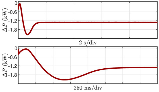
Figure 17. Test Case II: NLC $\Delta P$ value obtained with “virtual $V_{\mathrm{C}}^2$ control”.

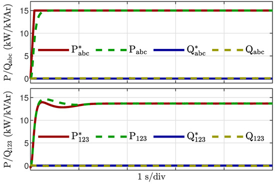
Figure 18. Test Case II: Comparison of ($P_{\mathrm{abc}}^{*},Q_{\mathrm{abc}}^{*},P_{123}^{*}$ and $P_{123}^{*}$) vs. measurements under NLC modulation.

Correspondingly, the performance assessment of “virtual $V_{\mathrm{C}}^2$ controller” under the PD–SPWM modulation strategy is shown in Figure 19. After the transient behavior of $\Delta P$ trace, the controller reaches steady–state in about 1.4 s, with a value of 1.317kW. At the same time, it provides active power reference for the three–phase AC system {123}.

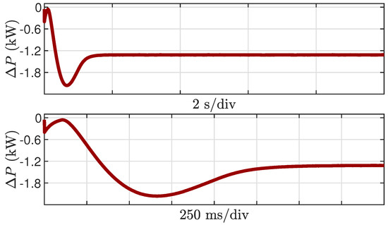
Figure 19. Test Case II: NLC $\Delta P$ value obtained with “virtual $V_{\mathrm{C}}^2$ control”.

This value of $\Delta P$ agrees with active power reference $P_{123}^{*}$ and its measurement, as it is illustrated in Figure 20. Furthermore, it can be stated that both traces of $P_{123}^{*}$ and $P_{123}$ are practically attached to each other. This indicates the performance of the “virtual $V_{\mathrm{C}}^2$ controller”. Under the above circumstances, the Hexverter–based system seems to perform with a value of $\eta =$ 91.22 efficiency.

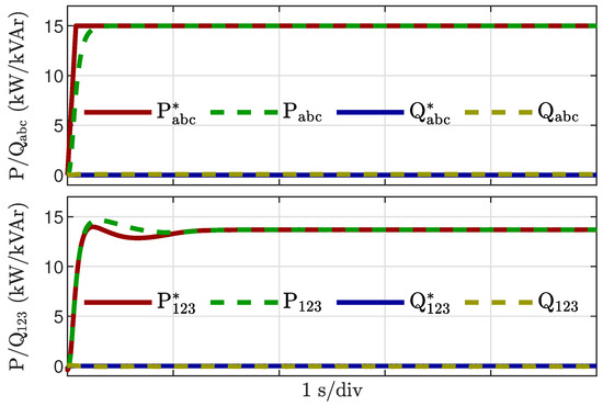
Figure 20. Test Case II: Comparison of ($P_{\mathrm{abc}}^{*},Q_{\mathrm{abc}}^{*},P_{123}^{*}$ and $P_{123}^{*}$) vs. measurements under PD–SPWM.

In summary, by comparing the results obtained from Test Cases I and II, the Hexverter-based system seems to be more efficient when the NLC modulation technique is utilized.

9. Detailed Assessment of Harmonic Spectrum and Total Harmonic Distortion of Voltages and Currents

The total harmonic distortion (THD) of any single phase waveform can be estimated by Equation (29):

$$\begin{array}{c}\hfill \mathrm{THD}=\frac{\sqrt{\sum _{k=2}^{\infty }{\mathrm{h}}_k^2}}{{\mathrm{h}}_1},\end{array}$$

(29)

where ${\mathrm{h}}_1$ accounts for the amplitude of the fundamental frequency, and ${\mathrm{h}}_k$ stands for any harmonic’s amplitude multiple of the fundamental frequency.

9.1. Single–Phase Voltage THD Assessment under NLC

Five cycles of single–phase voltage $v_{\mathrm{a}}$ are depicted in the top–left section of Figure 21. This voltage is measured at Hexverter’s terminals labeled as ${\mathrm{PCC}}_{\mathrm{abc}}$ (see Figure 1). Its frequency, magnitude, and phase are compliant with simulation parameters. Moreover, the harmonic content of $v_{\mathrm{a}}$ is assessed and illustrated in the bottom–left of Figure 21. A set of 160 harmonics labeled as ${\mathrm{h}}_{\mathrm{a},k}$ are shown. As expected, its magnitudes are monotonically decreasing as its harmonic order increases. Its THD is then calculated and equal to 2.21%. Harmonic’s number 29th = 1450 Hz and 31th = 1550 Hz are the most representative, featuring a magnitude of approximately 0.30%.

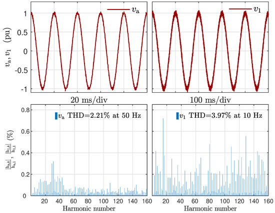
Figure 21. Spectrum of $v_{\mathrm{a}},v_1$ and THD calculations, when NLC modulation technique is utilized.

In the same fashion, five cycles of single–phase voltage $v_1$ are shown at the top–right section of Figure 21. This voltage is being measured at Hexverter’s terminals labeled as ${\mathrm{PCC}}_{123}$ (see Figure 1). By a simple inspection of Figure 21, $v_1$ looks more distorted compared to $v_{\mathrm{a}}$. This claim is consistent with the evaluation of $v_1$ harmonic content, which generates a value of 3.97% THD. A set of 160 harmonics labeled as ${\mathrm{h}}_{1,k}$ are shown in the bottom–right section of Figure 21. Notice that its magnitudes are monotonically decreasing as its harmonic order increases. In this case, harmonic’s number 15th = 150 Hz, 79th = 790 Hz, and 129th = 1290 Hz are the most representative, they feature magnitudes of 0.7%, 0.5%, and 0.55%, respectively.

9.2. Single–Phase Voltage THD Assessment under PD–SPWM

Five cycles of single–phase voltage $v_{\mathrm{a}}$ are shown in the top–left section of Figure 22. Correspondingly, the top–right section of the same figure shows five cycles of single–phase voltage $v_1$. Both voltage waveforms were measured at each PCC, respectively. The harmonic distortion measurement of single phase voltage $v_{\mathrm{a}}$ indicates a THD value = 2.50%. It is 13.2% higher in comparison to the THD value obtained by NLC modulation. Similarly, a THD value of $v_1$ equal to 3.98% is calculated. This former number indicates that, independently of the modulation technique, almost no difference regarding the THD value of $v_1$ can be observed. Be aware that a harmonic number 15th = 150 Hz, feature the highest magnitude (0.7% and 0.6%, respectively) under both modulation techniques.

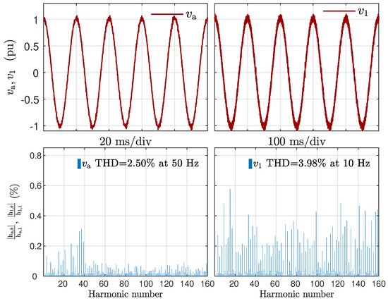
Figure 22. Spectrum of $v_{\mathrm{a}},v_1$ and THD results when PD–SPWM modulation technique is utilized.

9.3. Single–Phase Current THD Assessment under NLC

Single–phase current $i_{\mathrm{a}}$ is depicted in the top–left section of Figure 23. This current shows an amplitude of 10 Amperes, which, in turn, is compliant with simulation parameters. Its harmonic content is evaluated and shown in bottom–left section of Figure 23. The THD calculation indicates a number equal to 2.27%. Low–order harmonics, less than 3000 Hz, are the most representative featuring a highest magnitude of 0.46%. A similar trace is shown to indicate $i_1$ in the top–right section of Figure 23. As expected, this current feature an amplitude of nearly 10 Amperes. Its harmonic content corresponds to a value of 2.94%. Harmonics number $7\mathrm{th}$, $17\mathrm{th}$ and $35\mathrm{th}$ are the more representative ones, featuring magnitudes fairly close to 0.7%.

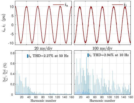
Figure 23. Spectrum of $i_{\mathrm{a}},i_1$ and THD calculations, when NLC modulation technique is utilized.

9.4. Single–Phase Current THD Assessment under PD–SPWM

Single–phase current $i_{\mathrm{a}}$ is depicted in the top–left section of Figure 24. Likewise, the top–right section of Figure 24 shows a single–phase current $i_1$. Both traces were measured at each PCC. The harmonic distortion computation of single–phase currents indicate THD values of 3.19% and 4.52%, respectively. THD values of PD–SPWM are higher than NLC in 40.6% and 54% each. Be aware that $i_1$ harmonic number $5\mathrm{th}$ = 50 Hz features the highest amplitude of 2.3% under PD–SPWM.

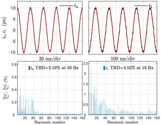
Figure 24. Spectrum of $i_{\mathrm{a}},i_1$ and THD results, when PD–SPWM modulation technique is utilized.

In summary, all the THD values obtained out of the PSCAD/EMTDC simulations are compliant with international standards IEEE 519 [13] and IEC61000–3–2 [14]. Moreover, it seems that the NLC modulation strategy outperforms the PD–SPWM modulation technique when the THD of synthesized waveforms is considered. In future work, some THD values can be reduced to a minimum by properly implementing modulation techniques such as harmonic elimination and selective harmonic elimination.

10. Conclusions

In this manuscript, the operational principle of the direct AC–AC multilevel power converter “Hexverter” was presented. The subsystems (i) branch current controller performing in a unified two–frequency $dq$ framework and (ii) a proposed “virtual $V_{\mathrm{C}}^2$ controller” were integrated to a power converter setup composed of (a) a modulator, (b) a voltage balancing algorithm, and (c) the Hexverter system. The results obtained suggest that the control scheme is able to regulate the Hexverter–based system under both modulation strategies. Moreover, an assessment of total harmonic distortion of AC three–phase voltages and currents was thoroughly developed. It seems that the NLC modulation strategy outperforms the PD–SPWM modulation technique. For instance, the THD of $v_{\mathrm{a}}$ is 13.2% higher under PD–SPWM than under NLC. Likewise, THD of $i_1$ is 54% higher under PD–SPWM than under NLC. Be aware, all the THD values obtained out of PSCAD/EMTDC simulations are compliant with international standards IEEE 519 [13] and IEC61000–3–2 [14]. Validations of proposed “virtual $V_{\mathrm{C}}^2$ control” were presented. According to the results obtained, the “virtual $V_{\mathrm{C}}^2$ controller” was able to accurately determine the active power loss of the Hexverter–based system. Furthermore, by assessing the $\Delta P$ values of both modulation techniques and under the scenarios of Test Case I and II, the nearest–level control technique yielded superior efficiency. The experimental validation of the analysis presented herein is currently under investigation. The results will be published as they become available.

References

- Baruschka, L.; Mertens, A. Transformatorloser Direktumrichter. German Patent DE102010013862A1, 1 April 2010. [Google Scholar]
- Baruschka, L.; Mertens, A. A New 3–Phase Direct Modular Multilevel Converter. In Proceedings of the 2011 14th European Conference on Power Electronics and Applications, Birmingham, UK, 30 August–1 September 2011. [Google Scholar]
- Baruschka, L.; Mertens, A. A New Three–Phase AC/AC Modular Multilevel Converter With Six Branches in Hexagonal Configuration. IEEE Trans. Ind. Appl. 2013, 49, 1400–1410. [Google Scholar] [CrossRef]
- Wan, Y.; Liu, S.; Jiang, J. Multivariable Optimal Control of a Direct AC/AC Converter under Rotating dq Frames. J. Power Electron. 2013, 13, 419–428. [Google Scholar] [CrossRef] [Green Version]
- Karwatzki, D.; Baruschka, L.; von Hofen, M.; Mertens, A. Optimised Operation Mode for the Hexverter Topology Based on Adjacent Compensating Power. In Proceedings of the 2014 IEEE Energy Conversion Congress and Exposition (ECCE), Pittsburgh, PA, USA, 14–18 September 2014; pp. 5399–5406. [Google Scholar]
- Karwatzki, D.; Baruschka, L.; Kucka, J.; von Hofen, M.; Mertens, A. Improved Hexverter Topology with Magnetically Coupled Branch Inductors. In Proceedings of the 2014 16th European Conference on Power Electronics and Applications, Lappeenranta, Finland, 26–28 August 2014; pp. 1–10. [Google Scholar]
- Karwatzki, D.; Baruschka, L.; von Hofen, M.; Mertens, A. Branch Energy Control for the Modular Multilevel Direct Converter Hexverter. In Proceedings of the 2014 IEEE Energy Conversion Congress and Exposition (ECCE), Pittsburgh, PA, USA, 14–18 September 2014; pp. 1613–1622. [Google Scholar]
- Baruschka, L.; Karwatzki, D.; von Hofen, M.; Mertens, A. Low–Speed Drive Operation of the Modular Multilevel Converter Hexverter Down to Zero Frequency. In Proceedings of the 2014 IEEE Energy Conversion Congress and Exposition (ECCE), Pittsburgh, PA, USA, 14–18 September 2014; pp. 5407–5414. [Google Scholar]
- Hamasaki, S.I.; Okamura, K.; Tsubakidani, T.; Tsuji, M. Control of Hexagonal Modular Multilevel Converter for 3–phase BTB System. In Proceedings of the 2014 International Power Electronics Conference (IPEC—Hiroshima 2014—ECCE ASIA), Hiroshima, Japan, 18–21 May 2014; pp. 3674–3679. [Google Scholar]
- Tsuruta, R.; Hosaka, T.; Fujita, H. A New Power Flow Controller Using Six Multilevel Cascaded Converters for Distribution Systems. In Proceedings of the 2014 International Power Electronics Conference (IPEC—Hiroshima 2014—ECCE ASIA), Hiroshima, Japan, 18–21 May 2014; pp. 1350–1356. [Google Scholar]
- Karwatzki, D.; Baruschka, L.; Mertens, A. Survey on the Hexverter Topology—A Modular Multilevel AC/AC Converter. In Proceedings of the 2015 9th International Conference on Power Electronics and ECCE Asia (ICPE-ECCE Asia), Seoul, Korea, 1–5 June 2015; pp. 1075–1082. [Google Scholar]
- Karwatzki, D.; von Hofen, M.; Baruschka, L.; Mertens, A. Operation of Modular Multilevel Matrix Converters with Failed Branches. In Proceedings of the IECON 2014—40th Annual Conference of the IEEE Industrial Electronics Society, Dallas, TX, USA, 29 October–1 November 2014; pp. 1650–1656. [Google Scholar]
- IEEE Standards Association. Recomended Practice and Requirements for Harmonic Control in Electric Power Systems; IEEE: Piscataway, NJ, USA, 2014. [Google Scholar]
- Electromagnetic Compatibility (EMC). IEC Standard 61000–3–2:2018; IEC: Geneva, Switzerland, 2018. [Google Scholar]
- Robles-Campos, H.R.; Mancilla-David, F. A comparative evaluation of modulation strategies for Hexverter—Based Modular Multilevel Converters. In Proceedings of the 2019 IEEE International Conference on Industrial Technology (ICIT), Melbourne, Australia, 13–15 February 2019; pp. 1465–1470. [Google Scholar]
- Yazdani, A.; Iravani, R. Voltage–Sourced Converters in Power Systems: Modeling, Control, and Applications. In Voltage–Sourced Converters in Power Systems: Modeling, Control, and Applications; IEEE Pres/Wiley: Hoboken, NJ, USA, 2010. [Google Scholar]
- Robles-Campos, H.R.; Mancilla-David, F. A control scheme in the dq reference frame for Hexverter–based systems. In Proceedings of the 2019 North American Power Symposium (NAPS), Wichita, KS, USA, 13–15 October 2019; pp. 1–6. [Google Scholar]
- Qin, J.; Saeedifard, M. Reduced Switching–Frequency Voltage–Balancing Strategies for Modular Multilevel HVDC Converters. IEEE Trans. Power Deliv. 2013, 28, 2403–2410. [Google Scholar] [CrossRef]
- Konstantinou, G.; Pou, J.; Ceballos, S.; Darus, R.; Agelidis, V.G. Switching Frequency Analysis of Staircase—Modulated Modular Multilevel Converters and Equivalent PWM Techniques. IEEE Trans. Power Deliv. 2016, 31, 28–36. [Google Scholar] [CrossRef] [Green Version]
- Hu, P.; Jiang, D. A Level-Increased Nearest Level Modulation Method for Modular Multilevel Converters. IEEE Trans. Power Electron. 2015, 30, 1836–1842. [Google Scholar] [CrossRef]
- Knuth, D. The Art of Computer Programming. In The Art of Computer Programming, 3rd ed.; Addison-Wesley: Boston, MA, USA, 1997. [Google Scholar]
- PSCAD/EMTDC Software Platform; Version 4.6.3; Manitoba HVDC Research Centre: Manitoba, CA, USA, 2018.
Publisher’s Note: MDPI stays neutral with regard to jurisdictional claims in published maps and institutional affiliations. |
© 2022 by the authors. Licensee MDPI, Basel, Switzerland. This article is an open access article distributed under the terms and conditions of the Creative Commons Attribution (CC BY) license (https://creativecommons.org/licenses/by/4.0/).