Effective Volt/var Control for Low Voltage Grids with Bulk Loads

Abstract

This paper investigates the voltage and reactive power control problem in low voltage grids with connected prosumers and bulk loads. The X(U) local control, which maintains the voltage at the feeders’ ends within a predefined band, and its combination with Q-Autarkic customer plants are the most effective and reliable strategies in grids with high prosumer share. However, these strategies may need adaptations to guarantee voltage limit compliance when bulk loads, such as electric vehicle parking garages and community-owned photovoltaic systems, are connected to the low voltage feeders. This paper extends the X(U) local control concept to involve bulk loads in Volt/var control and investigates the resulting load flows in different real low voltage grids. The results show that the extended control arrangement reliably removes all voltage limit violations by deteriorating the effectiveness of the original X(U) local control arrangement: reactive power flows and equipment loading within the low voltage grids are increased.

1. Introduction

Decreasing costs of renewable energy sources, advances in digitalization, and growing opportunities for electrification drive significant changes in electric power systems [1]. The share of renewable energy sources such as photovoltaic (PV) and wind turbine systems is drastically increasing [2], and a widespread charging infrastructure for electric vehicles (EV) is being erected to promote the decarburization of the transport sector [3]. Energy communities arise that strengthen energy democracy by involving citizens in participative decision-making and collective ownership of electric facilities [4,5]. These communities are expected to stimulate investments in local power systems and boost the emergence of distributed energy resources. Collective financing allows implementing large projects, such as installing producer and storage units with capacities up to several 100 kWp at the low voltage (LV) level.

The rapidly increasing share of distributed energy resources challenges the operation of distribution grids in terms of power quality, protection, and stability [6,7,8]. Maintaining compliance with the legal voltage limits constitutes a major challenge for the operation of smart grids [9]. In many cases, the active power transfer capability of the grid is primarily restricted by voltage and not by thermal limits [10,11]. Coordinated or local Volt/var control may be used to mitigate voltage variations and increase the grid’s transfer capacity by manipulating the reactive power (Q) flows and transformer tap positions. Coordination supports optimal system operation but causes additional costs for distributed data collection and central data processing [12]. The related data exchanges pose severe challenges for information and communication technology systems and impair data privacy. Meanwhile, local controls are cheap to implement as they do not require widespread communication [13,14,15], but they provoke uncontrolled power flows within the grid [16]. Today, local controls are commonly applied to control the voltage at the LV level.

Local controls may be used to adjust the tap positions of distribution transformers (DTR) [17] and the reactive power contributions of producer and storage units [18,19] as well as reactive power devices (RPD) such as mechanically switched capacitors. At present, most European DTRs do not possess on-load tap changers but their tap positions are fixed and can only be modified after de-energization. Furthermore, on-load tap changers are slow to operate and sensitive to the number of tap operations. They cannot react appropriately to the voltage fluctuations caused by the intermittent PV injections. Temporary voltage limit violations and unnecessary tap operations are the consequence, thus jeopardizing the electrical equipment and shortening the transformers’ durability [20]. Therefore, this article focuses on reactive power control and does not investigate voltage control by on-load tap changers in distribution substations.

cosφ(P) and Q(U) are the most renowned local control schemes for PV inverters [21]. Several studies refine these schemes by considering more local variables [21,22,23,24], such as active and reactive power consumption of household appliances and the grid’s R/X-ratio prevailing at their connection points. All these strategies use customer-owned inverters to control the voltage at the LV level. Meanwhile, ref. [25] proposes the installation of RPDs equipped with X(U) local controls that maintain the voltages at the LV feeder ends within a predefined band. This control strategy may be combined with Q-Autarkic Customer Plants (CP), which use their PV inverters or other var sources to supply the reactive power demand of the corresponding household appliances locally [26]. Such CPs do not exchange any reactive power with the LV grid.

The simulation study presented in [25] demonstrates the increased effectiveness of the X(U) local control and its combination with Q-Autarkic CPs compared to the Q(U) and cosφ(P) local controls of distributed inverters. However, the analysis is restricted to residential EV chargers and rooftop PV systems and does not investigate the effect of bulk consumers (BC) and bulk producers (BP). In the presence of such bulk loads, voltage limit violations may occur somewhere along the feeder even when the X(U) local control maintains acceptable voltages at the feeders’ ends.

This paper analyses the ability of the X(U) local control in combination with CP_Q-Autarky to maintain acceptable voltages when bulk loads such as EV parking garages and community-owned PV systems are connected close to the feeder middle. It focuses on Austrian LV grids and uses the voltage limits of ±10% around the nominal voltage that are stipulated by the Austrian grid code [27]. The X(U) local control concept is extended to maintain acceptable voltages throughout the entire LV feeder length by implementing the X(U) control scheme not only at the feeders’ ends but also into the bulk loads.

Section 2 describes the state-of-the-art reactive power control at the LV level in detail, and presents the extended X(U) local control arrangement introduced in this paper. All investigated control arrangements, the used power system models and load flow calculation software, and the simulated scenarios are described in detail in Section 3. Section 4 presents the calculated grid behavior, and Section 5 discusses the effectiveness of the extended control arrangement. Conclusions are drawn in Section 6.

2. Reactive Power Control in Low Voltage Grids

This section reviews the state-of-the-art concerning reactive power local control in LV grids, discusses the shortcomings of the recently introduced X(U) local control, and presents a new approach to resolve these shortcomings.

2.1. Volt/Watt and Volt/var Interrelations

The power flows through the grid affect the node voltages and vice versa. These interrelations are illustrated based on the two-bus system shown in Figure 1. Therein, ${\underset{\_}{S}}_1$ and ${\underset{\_}{S}}_2$ denote the complex apparent power flowing into and out of the complex impedance $\underset{\_}{Z}$, and ${\underset{\_}{U}}_1$ and ${\underset{\_}{U}}_2$ are the complex voltages at buses one and two.

Equations (1)–(5) describe the apparent power flows, impedance, and voltages, wherein $P_2$, $Q_2$ are the active and reactive power flowing out of the impedance; $R$, $X$ are the resistance and reactance; $U_1, {\delta }_1$ are the magnitude and angle of the voltage at bus one; $U_2, {\delta }_2$ are the magnitude and angle of the voltage at bus two; and $\delta$ is the voltage angle difference between buses one and two.

$${\underset{\_}{S}}_2=P_2+j{Q}_2,$$

(1)

$$\underset{\_}{Z}=R+jX,$$

(2)

$${\underset{\_}{U}}_1=U_1·{\mathrm{e}}^{j{\delta }_1},$$

(3)

$${\underset{\_}{U}}_2=U_2·{\mathrm{e}}^{j{\delta }_2},$$

(4)

$$\delta ={\delta }_2-{\delta }_1,$$

(5)

These definitions allow formulating the voltage drop equation as in Equation (6).

$$U_1·\cos \left(\delta \right)-U_2=\left(R{P}_2+X{Q}_2\right)/U_2.$$

(6)

Neglecting the voltage angle difference between both nodes ($\cos \delta \approx 1$), which is justified in distribution grids [28], allows simplifying the voltage drop equation according to Equation (7), wherein $\Delta U$ is the voltage magnitude difference between buses on and two.

$$\Delta U=U_1-U_2\approx \left(R{P}_2+X{Q}_2\right)/U_2.$$

(7)

According to Equation (7), the voltage rise caused by an active power injection at bus two may be mitigated by a simultaneous reactive power absorption, and vice versa. While the active power’s effect depends on the resistance, the effect of the reactive power depends on the reactance. Based on this principle, reactive power control allows compensating the voltage variations caused by the active power transfer through the grid.

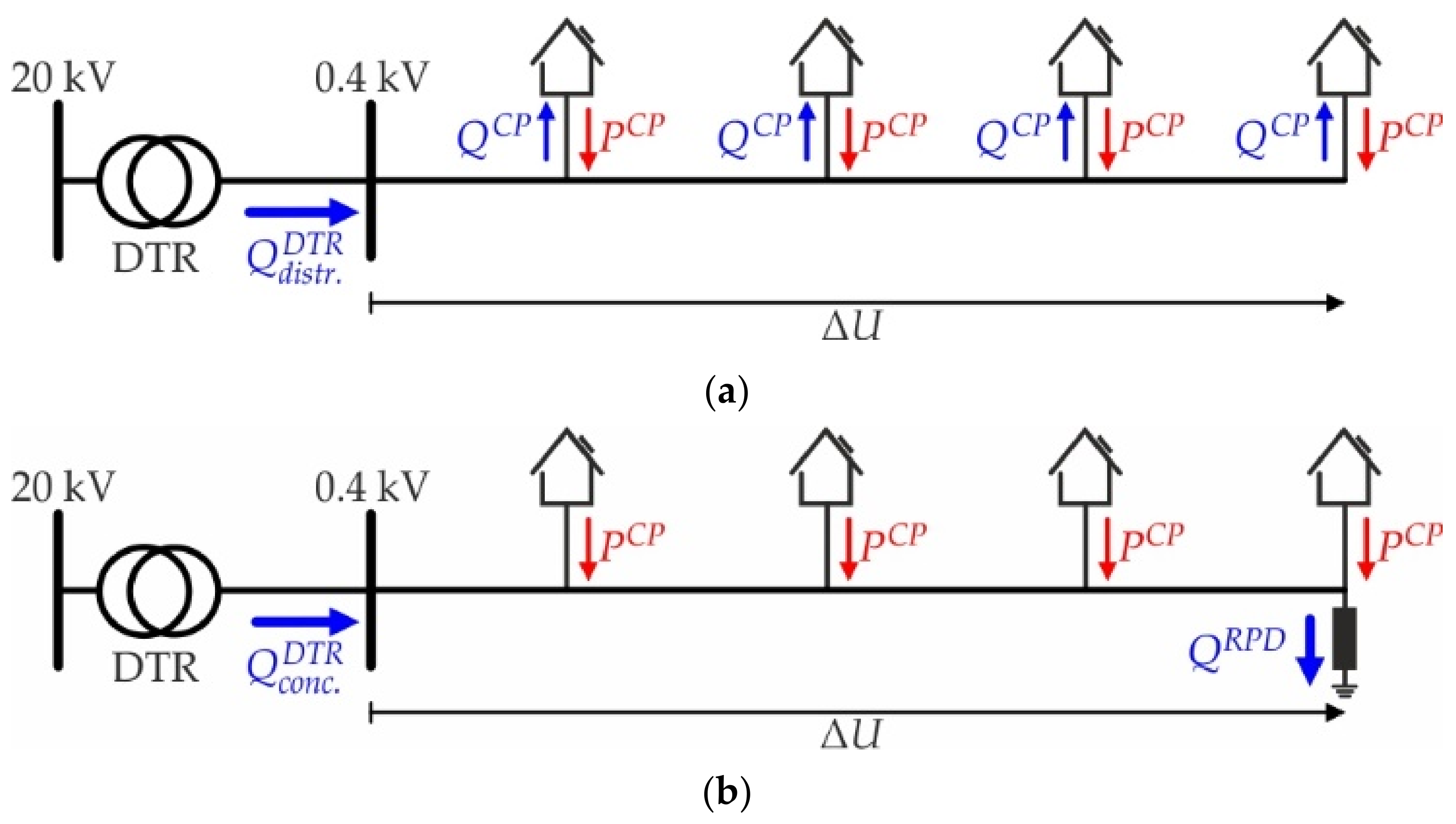
2.2. Effectiveness of Volt/var Control

In general, reactive power may be contributed at various locations along the LV feeders. According to Equation (7), its effect on the feeder voltage depends on the corresponding injection and absorption points. References [29,30] distinguish between distributed and concentrated var contributions and analyze their effects on the feeders’ voltage profiles. Distributed reactive power contributions are defined as var contributions at various nodes distributed throughout the length of the feeder, while the concentrated reactive power contribution refers to one var contribution close to the feeder end. Both cases are illustrated in Figure 2, where the distributed CPs inject active power ($P^{CP}$) into the grid. In Figure 2a, the CPs also consume reactive power, thus partly compensating the voltage rise caused by their active power injections. Here, the reactive power $Q_{distr.}^{DTR}$ flows into the LV feeder. Meanwhile, in Figure 2b, the CPs do not contribute any reactive power. Instead, an RPD connected at the feeder end consumes reactive power ($Q^{RPD}$) to mitigate the voltage rise, leading to the reactive power flow $Q_{conc.}^{DTR}$ at the feeder beginning.

The analyses conducted in the mentioned references show that the concentrated var contribution is more effective than the distributed ones, as it provokes lower reactive power flows at the distribution substation level to achieve the same total voltage drop ($\Delta U$) over the LV feeder, i.e., $Q_{conc.}^{DTR}<Q_{distr.}^{DTR}$.

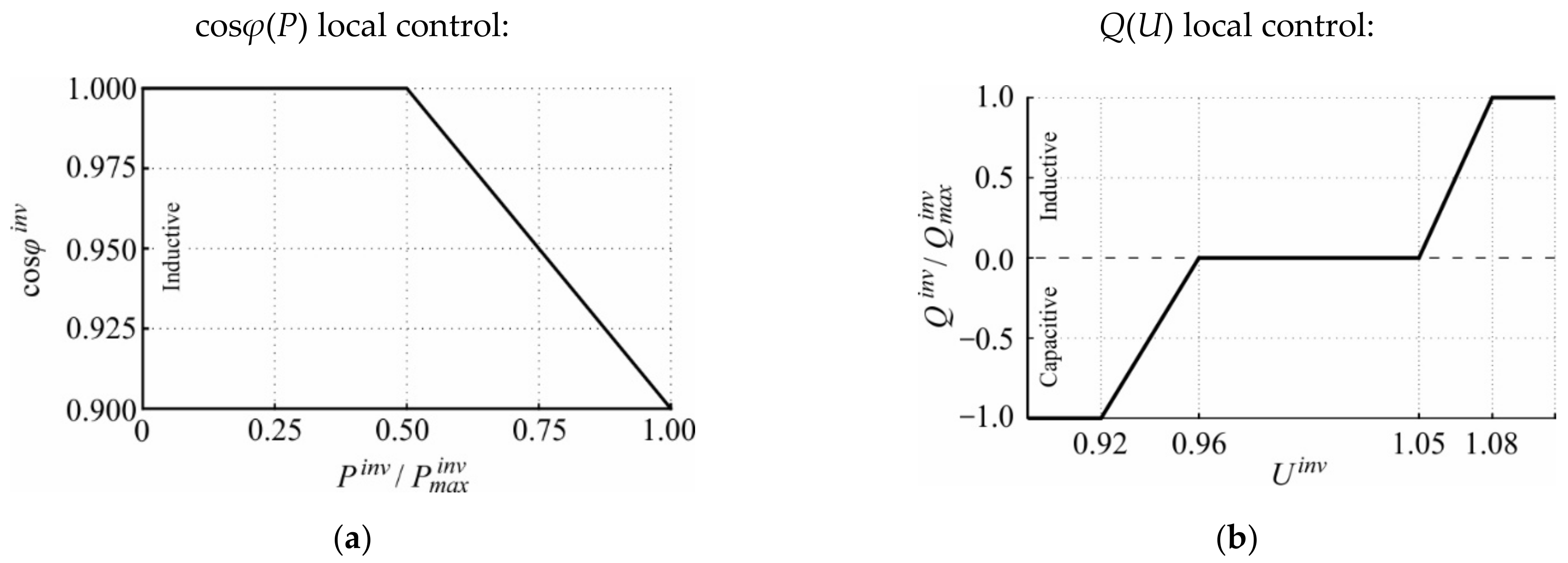
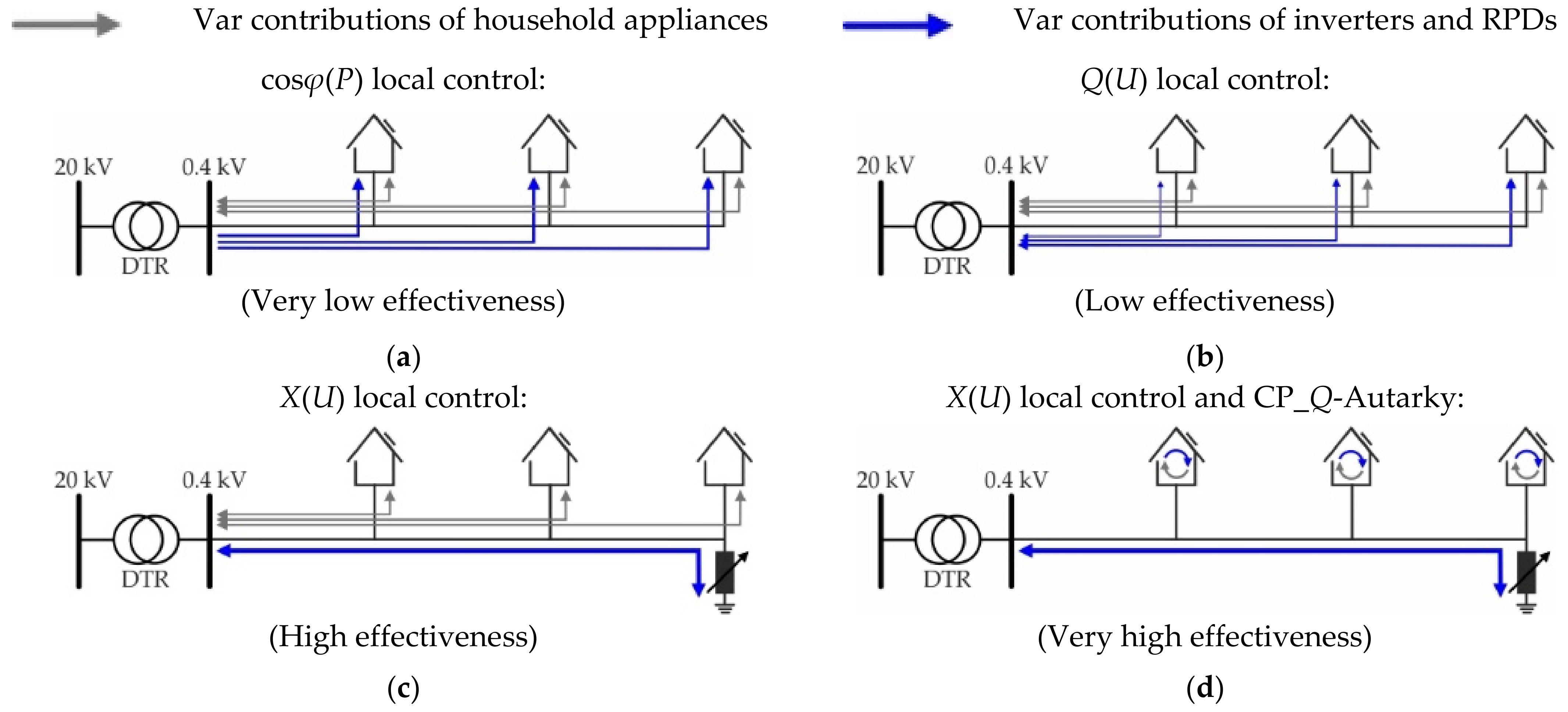
2.3. Local Volt/var Control Strategies

Figure 3a,b show the characteristics of the cosφ(P) and Q(U) local controls specified by the Austrian grid code [31]. Therein, $\cos {\phi }^{inv}$ is the inverter’s power factor; $P^{inv}$, $Q^{inv}$ are its active and reactive power exchanges with the grid; $P_{max}^{inv}$, $Q_{max}^{inv}$ are its maximal active and reactive power injections; and $U^{inv}$ is the voltage at its terminal. Usually, the inverters are over-dimensioned compared to the PV-modules to enable the operation with low power factor during peak production periods. While the cosφ(P)-controlled inverters consume reactive power depending on their active power injection, the Q(U)-controlled ones absorb or inject reactive power as functions of the local voltages. The X(U) local control strategy is illustrated in Figure 3c: The RPD connected at the LV feeder’s end maintains its local voltage between 0.91 and 1.09 p.u. Here, the customer-owned PV inverters are not used to control the voltage at the LV level.

2.3.1. Modeling in Load Flow Analysis

In load flow analysis, the X(U) local control strategy is modeled completely differently than the cosφ(P) and Q(U) schemes. The cosφ(P) and Q(U) local control strategies are modeled as ‘PQ-node elements’, which means that the active and reactive power contributions of the inverters are specified (constant active power and reactive power as functions of P and U, respectively). Meanwhile, the modeling of the X(U) scheme depends on the local voltage: For acceptable voltages, i.e., $0.91 \mathrm{p}.\mathrm{u}.<U<1.09 \mathrm{p}.\mathrm{u}.$, the X(U)-controlled device is modeled as a PQ-node element (P and Q are set to zero). When the voltage approaches the lower or upper limit, i.e., $U\le 0.91 \mathrm{p}.\mathrm{u}.$ or $U\ge 1.09 \mathrm{p}.\mathrm{u}.$, it is modeled as a ‘PV-node element’, which means that its active power and voltage magnitude are specified (P is set to zero and U is set to 0.91 and 1.09 p.u., respectively).

2.3.2. Effectiveness

The discussed control strategies provoke distinct reactive power flows, thus having different effects on the voltage profiles of the LV feeders. A high effectiveness of a Volt/var control means that the reactive power has a great effect on the voltage, i.e., $\left|\partial U/\partial Q\right|$ is large. Figure 4 illustrates the reactive power flows at the LV level resulting from these control strategies and indicates the increasing effectiveness from the cosφ(P) local control to the X(U) local control combined with CP_Q-Autarky.

In Figure 4a, the household appliances inject or absorb reactive power and the cosφ(P)-controlled PV inverters consume reactive power, provoking distributed var contributions along the LV feeder. In this case, all inverters consume the same amount of reactive power in relation to their rating. The results are strongly inhomogeneous reactive power flows through the LV feeder, i.e., large flows occur in the foremost line segment and small ones in the backmost line segment. This control setup is relatively ineffective due to the highly distributed character of the var contributions. When Q(U) local control is applied, the inverters connected at the beginning of the feeder absorb or inject less reactive power than those connected at the feeder end, Figure 4b. The var flows are less inhomogeneous compared to the setup with cosφ(P) local control, and therefore the solution is more effective. However, the reactive power contributions still have a highly distributed character. In Figure 4c, reactive power is absorbed by an X(U)-controlled RPD connected at the feeder end. The PV inverters do not contribute any reactive power, but the household appliances still provoke distributed var contributions. This setup further homogenizes the reactive power flows, leading to an improved effectiveness compared to the Q(U) local control. The most effective control strategy is shown in Figure 4d, where the X(U) local control is combined with Q-Autarkic CPs. The inverters fully compensate the reactive power exchanges between the CPs and the LV feeder, and the X(U) local control maintains acceptable voltages at the feeder end. As a result, only one concentrated var absorption appears at the feeder end, allowing for maximal effectiveness according to Section 2.2.

2.3.3. Economic Considerations

In contrast to cosφ(P) and Q(U), the X(U) local control requires the installation of costly RPDs with variable reactance. However, its superior effectiveness reduces the uncontrolled reactive power flows, thus increasing the utilization of the LV grids. Careful assessment must ensure the economic value of the X(U) local control for specific feeders.

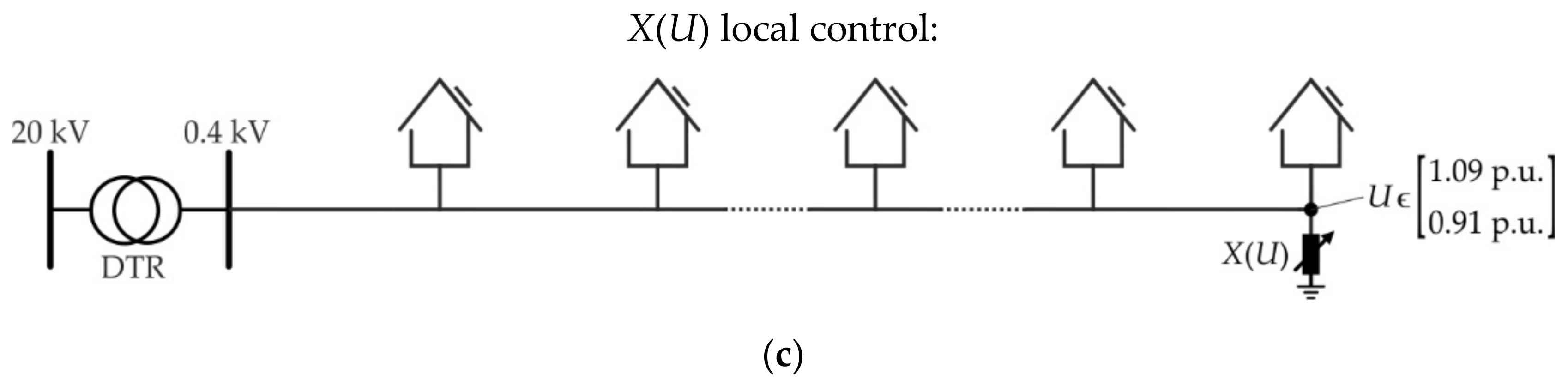
2.4. Shortcomings of the X(U) Local Control Scheme

Previous analysis showed that the X(U) local control and its combination with Q-Autarkic CPs are the most effective strategies to maintain acceptable voltages in LV grids that connect similar residential CPs with rooftop PV systems and EV chargers [25,30]. However, when bulk consumers and producers, such as EV parking garages and community-owned photovoltaic plants, are connected close to the LV feeder middle, these strategies may be insufficient to maintain acceptable voltages throughout the entire feeder length. Figure 5 illustrates this problem for both cases and the combination of X(U) local control with Q-Autarkic CPs. Active and reactive power contributions are marked in red and blue colors, respectively.

The three foremost CPs shown in Figure 5a inject active power due to their PV production, while the backmost one consumes active power. Their inverters or other var sources compensate the reactive power exchanges between the CPs and the LV grid. Meanwhile, the EV parking garage consumes excessive amounts of active power ($P^{BC}$), provoking a voltage drop between the distribution substation and its delivery point. In the rear part of the feeder, the voltage firstly increases due to the injection of the third CP and decreases again afterwards. Here, violations of the lower voltage limit occur in the middle part of the feeder although the X(U)-controlled RPD injects reactive power to maintain its local voltage at 0.91 p.u. The opposite behavior appears in Figure 5b, where the bulk injection ($P^{BP}$) of the community-owned PV plant provokes violations of the upper limit although the X(U) local control keeps the voltage at the feeder end at 1.09 p.u.

2.5. Extending the X(U) Local Control Scheme

The contribution of this paper is to extend the X(U) local control arrangement to eliminate the voltage limit violations in the middle part of the LV feeders. Therefore, the X(U) local control scheme is implemented not only at the LV feeders’ ends but also into the bulk loads. This extension is illustrated in Figure 6 for the case with a bulk consumer. Here, the parking garage injects reactive power to keep the voltage at its delivery point at or above 0.91 p.u. According to Equation (7), the additional reactive power injection $Q^{BC}$ increases the voltage in the middle part of the feeder, thus maintaining acceptable voltages throughout the entire feeder length. The analogous extension is made for the case with a bulk producer.

3. Materials and Methods

This study uses load flow simulations to analyze the effect of the state-of-the-art and extended X(U) local control arrangement in combination with Q-Autarkic CPs on the behavior of LV grids with connected bulk loads. Section 3.1, Section 3.2, Section 3.3 and Section 3.4 describe the investigated control arrangements, the used power system models and calculation software, and the defined scenarios.

3.1. Description of Volt/var Control Arrangements

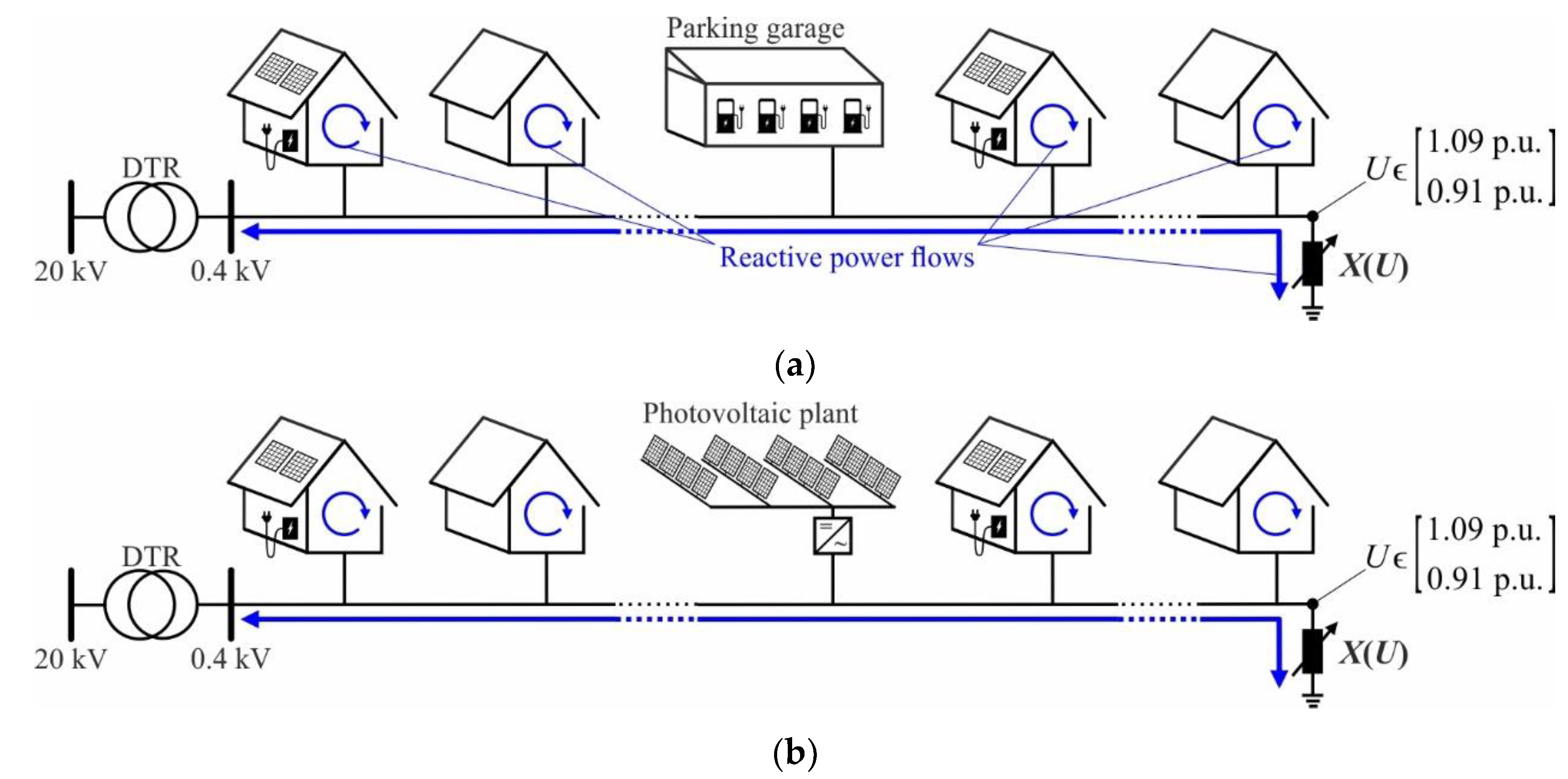
3.1.1. No Volt/var Control

Figure 7 overviews the arrangement without any Volt/var control. Besides various residential CPs, the LV feeder connects an EV parking garage in Figure 7a and a PV plant in Figure 7b. The garage and PV system do not contribute any reactive power when no Volt/var control is used. Additionally, PV systems and EV chargers connected at the CP level do not provide any reactive power. Therefore, the CPs exchange reactive power with the LV grid to cover the needs of their consuming devices, such as motor-driven, lighting, and switch-mode power supply devices.

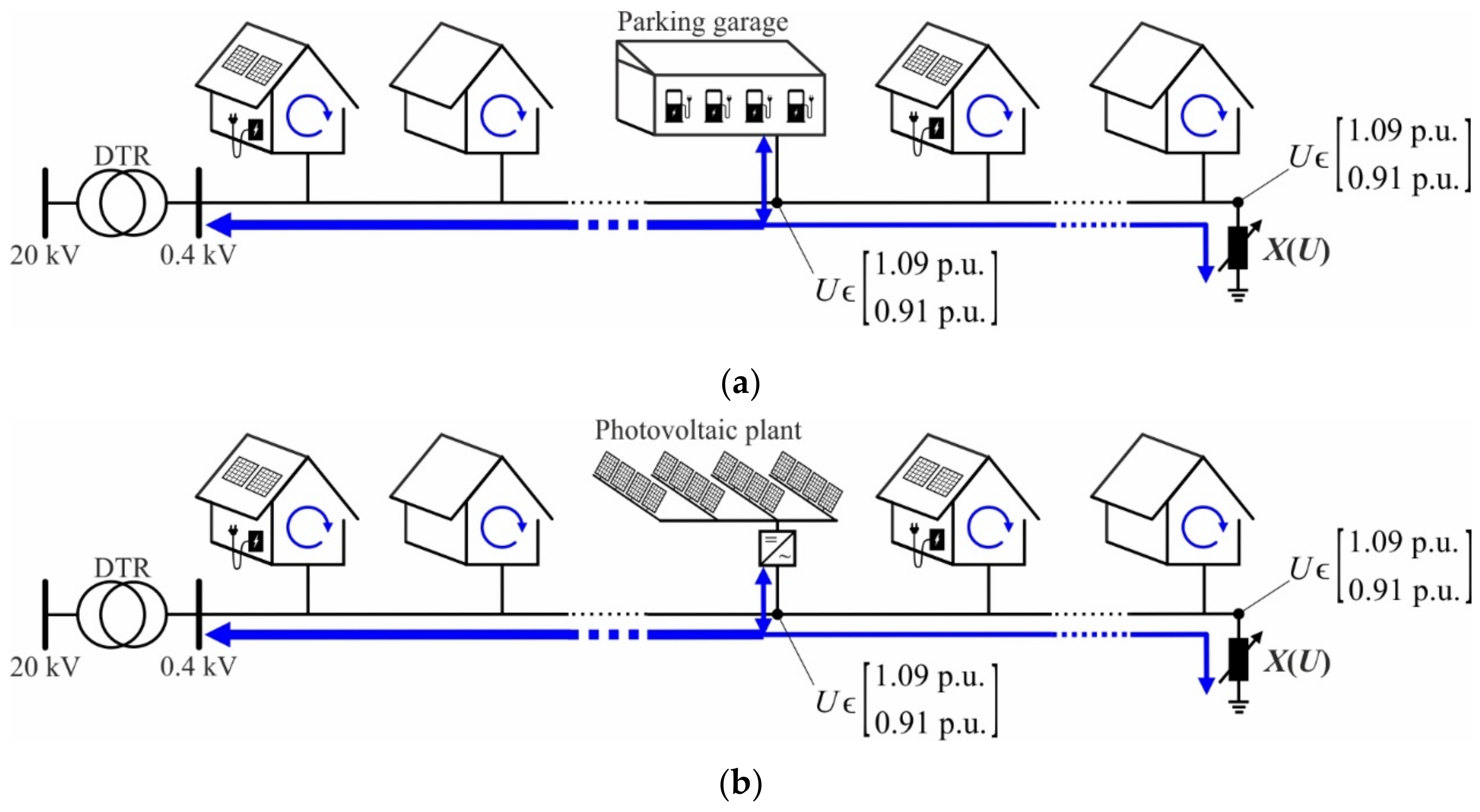
3.1.2. X(U) Local Control and CP_Q-Autarky

Figure 8a,b show the arrangement with X(U) local control and Q-Autarkic CPs for both bulk load types. Residential CPs supply the reactive power demand of their consuming devices locally, either by using the var capabilities of their rooftop PV systems and EV chargers or by using an additional var compensator. No reactive power is exchanged between the CPs and the LV grid. Furthermore, RPDs equipped with X(U) local control are connected close to the ends of the violating LV feeders, i.e., those feeders which may violate the upper or lower voltage limits. These devices absorb or inject the amount of reactive power required to maintain their terminal voltages between 0.91 and 1.09 p.u.

3.1.3. X(U)⁺ Local Control and CP_Q-Autarky

The arrangement with X(U) local control and Q-Autarkic CPs is extended in Figure 9a,b, where the X(U) control is additionally implemented at the bulk loads’ delivery points. This extension is denoted as ‘X(U)⁺ local control’. The necessary reactive power may be provided by the EV chargers, PV inverter, or an additional RPD.

3.2. Description of Models

The effect of the different control arrangements presented in Section 3.1 on the LV feeder voltages is investigated using steady-state models of residential CPs, bulk consumers and producers, and real LV grids. While real data are used for the LV grids, the models of the residential customer plants and bulk loads are synthesized to allow the investigation of very critical injection and consumption scenarios. Asymmetry is not considered.

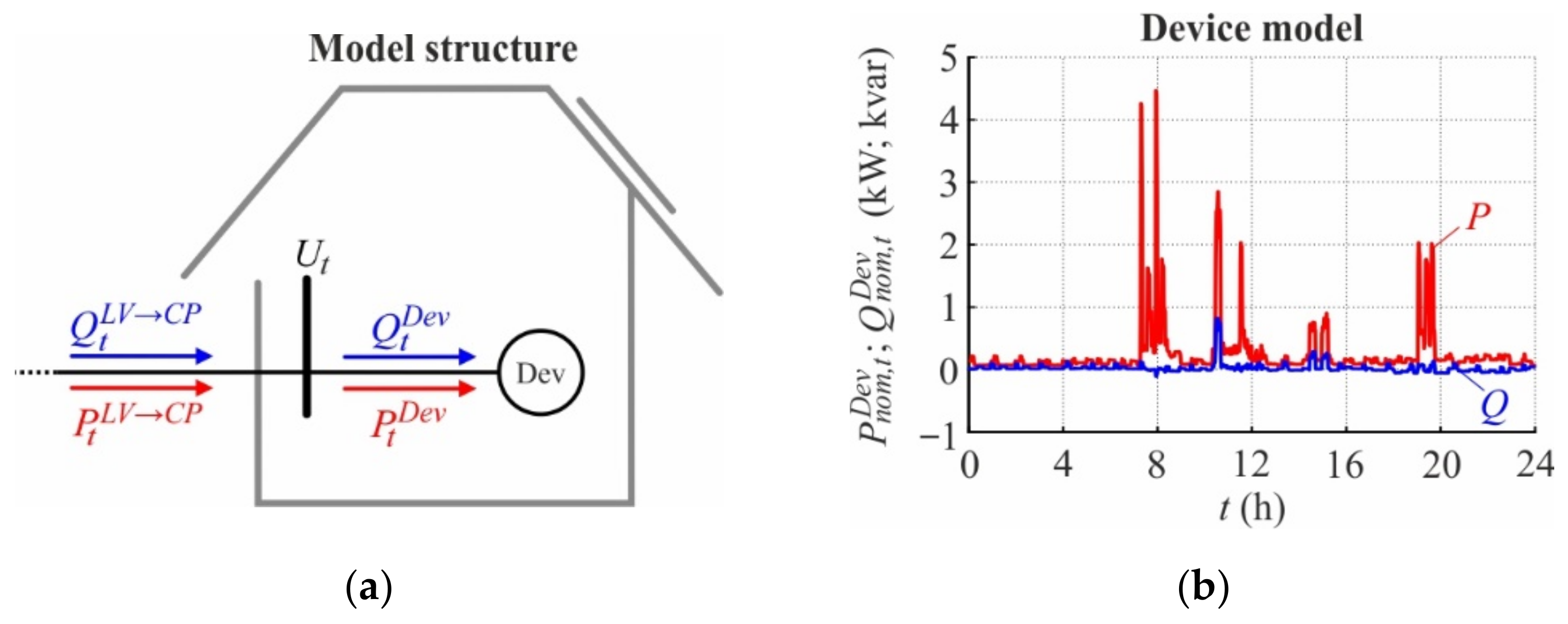
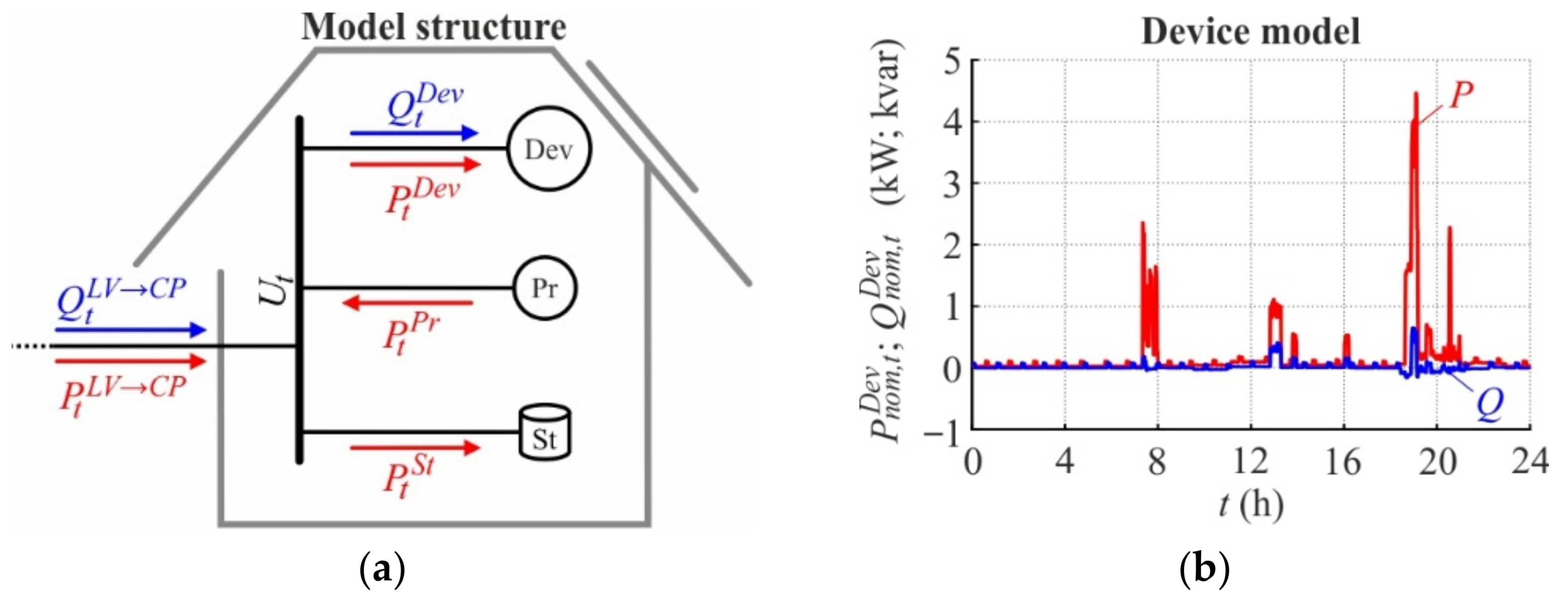
3.2.1. Residential Customer Plants

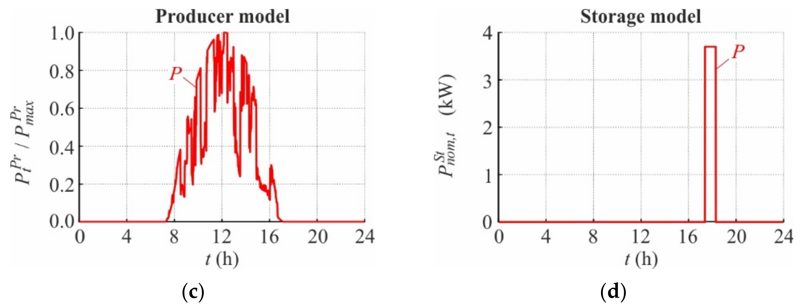
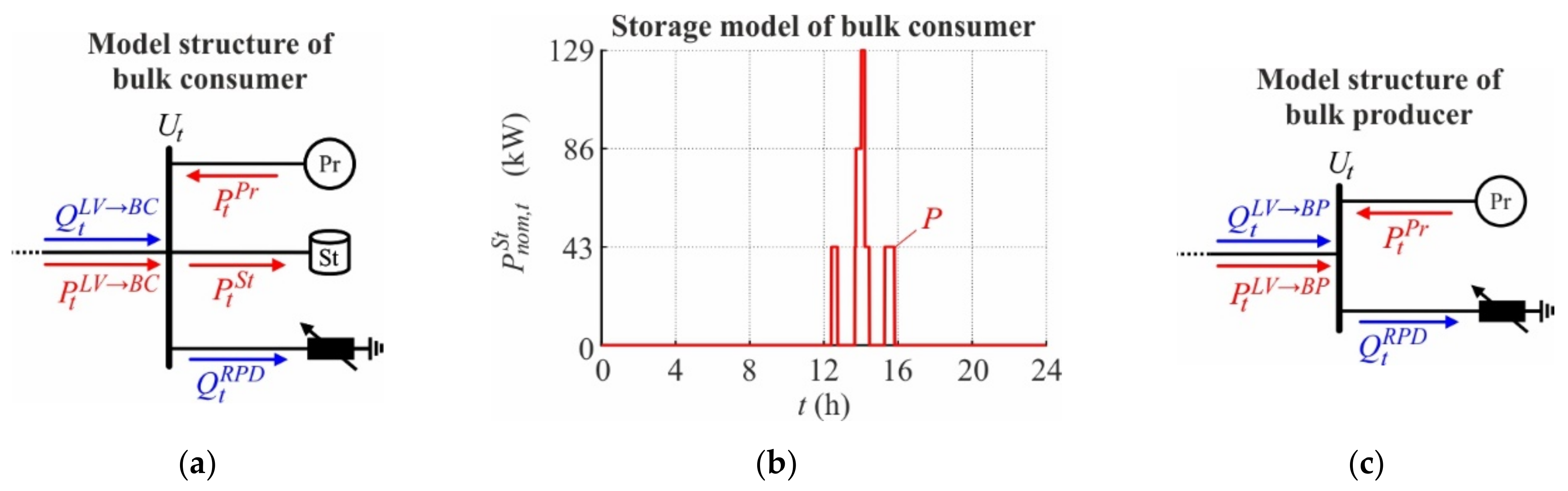
Two different types of residential customer plants are defined to reflect the limited penetration of rooftop PV systems and residential EV chargers: consumer and prosumer. Power losses at the CP level are neglected. This section overviews both models and the exact model data are provided in Appendix A.

As shown in Figure 10a, the residential consumer includes a device (Dev.) model representing the active ($P_t^{Dev}$) and reactive power ($Q_t^{Dev}$) behavior of all simultaneously used household appliances, such as motor-driven, lighting, and switch-mode power supply devices. It exchanges active ($P_t^{LV\to CP}$) and reactive power ($Q_t^{LV\to CP}$) with the LV grid. Individual consumption profiles, which are synthesized with the load profile generator [32], are used for the Dev.-model of each residential consumer. An example is shown in Figure 10b, wherein the active ($P_{nom,t}^{Dev}$) and reactive power ($Q_{nom,t}^{Dev}$) contributions at nominal voltage are drawn in red and blue colors, respectively. The actual power contributions depend on the local voltage ($U_t$) and are specified by the polynomial load model presented in [33]. This model describes the voltage dependency of modern residential consuming devices in New York City. Here, it is assumed that Austrian households use similar devices, so the same model parameters are used. CP_Q-Autarky is modeled by setting the reactive power contribution of the dev-model to zero ($Q_t^{Dev}=0, \forall t$). In reality, the LV→CP reactive power flow is eliminated by the PV inverter or another reactive power source. However, this simplified modeling of CP_Q-Autarky is valid as the losses at the CP level are neglected and the reactive power source is assumed to be sufficiently dimensioned.

Figure 11a shows that the model of the residential prosumer includes three components: the Dev.-model, the producer (Pr) model, and the storage (St) model.

The device component is modeled in the same way as the residential consumer’s one. Each prosumer has a PV system with a maximal active power production of $P_{max}^{Pr}=5 \mathrm{kW}$ represented by the Pr.-model, and an EV charger represented by the St.-model. While the production ($P_t^{Pr}$) of the PV system is modeled voltage-independently [34], the consumption ($P_t^{St}$) of the EV charger is modeled using the polynomial load model presented in [35]. Battery discharging is not considered in this study. Individual consumption profiles are synthesized with the load profile generator for the Dev.- and St.-models of each residential prosumer. Figure 11b,d provide examples for these profiles, wherein the EV charger’s active power consumption at a nominal voltage is denoted as $P_{nom,t}^{St}$. Meanwhile, the same production profile is used for all PV systems due to their proximity. This assumption is justified when the individual orientation and characteristics of PV modules and shading effects are neglected. The production profile shown in Figure 11c is created by considering the sudden appearance of clouds [36].

3.2.2. Bulk Loads

The effect of bulk consumption and production on the LV grid voltages is investigated by considering an EV parking garage with several quick chargers and a community-owned photovoltaic plant. Figure 12a presents the structure of the bulk consumer model: its active ($P_t^{LV\to BC}$) and reactive power ($Q_t^{LV\to BC}$) exchanges with the LV grid are determined by a Pr.-model representing a 40 kWp rooftop PV system, a St.-model representing several 43 kW quick chargers, and an RPD.

The voltage-independent injection of the PV system follows the production profile shown in Figure 11c. Meanwhile, the chargers are represented by a polynomial load model, and their consumption at nominal voltage is specified by the profile shown in Figure 12b. Five EV batteries are charged throughout the day, whereby three chargers are simultaneously active between 14:01 and 14:12, provoking a total active power absorption of around 129 kW during this interval. Battery discharging is not considered in this study. The RPD contributes reactive power depending on the local voltage only when the X(U)⁺ control arrangement is applied (see Section 2.3.1 and Section 3.1.3).

According to Figure 12c, the model of the bulk producer includes a Pr.-model and an RPD and exchanges active ($P_t^{LV\to BP}$) and reactive power ($Q_t^{LV\to BP}$) with the LV grid. The Pr.-model represents the PV plant with a maximal production of 100 kW and 50 kW in the urban and rural LV grid (see Section 3.2.3), respectively. Its actual production is determined by the profile shown in Figure 11c. Similarly to the model of the bulk consumer, the RPD contributes reactive power only when the X(U)⁺ control arrangement is applied.

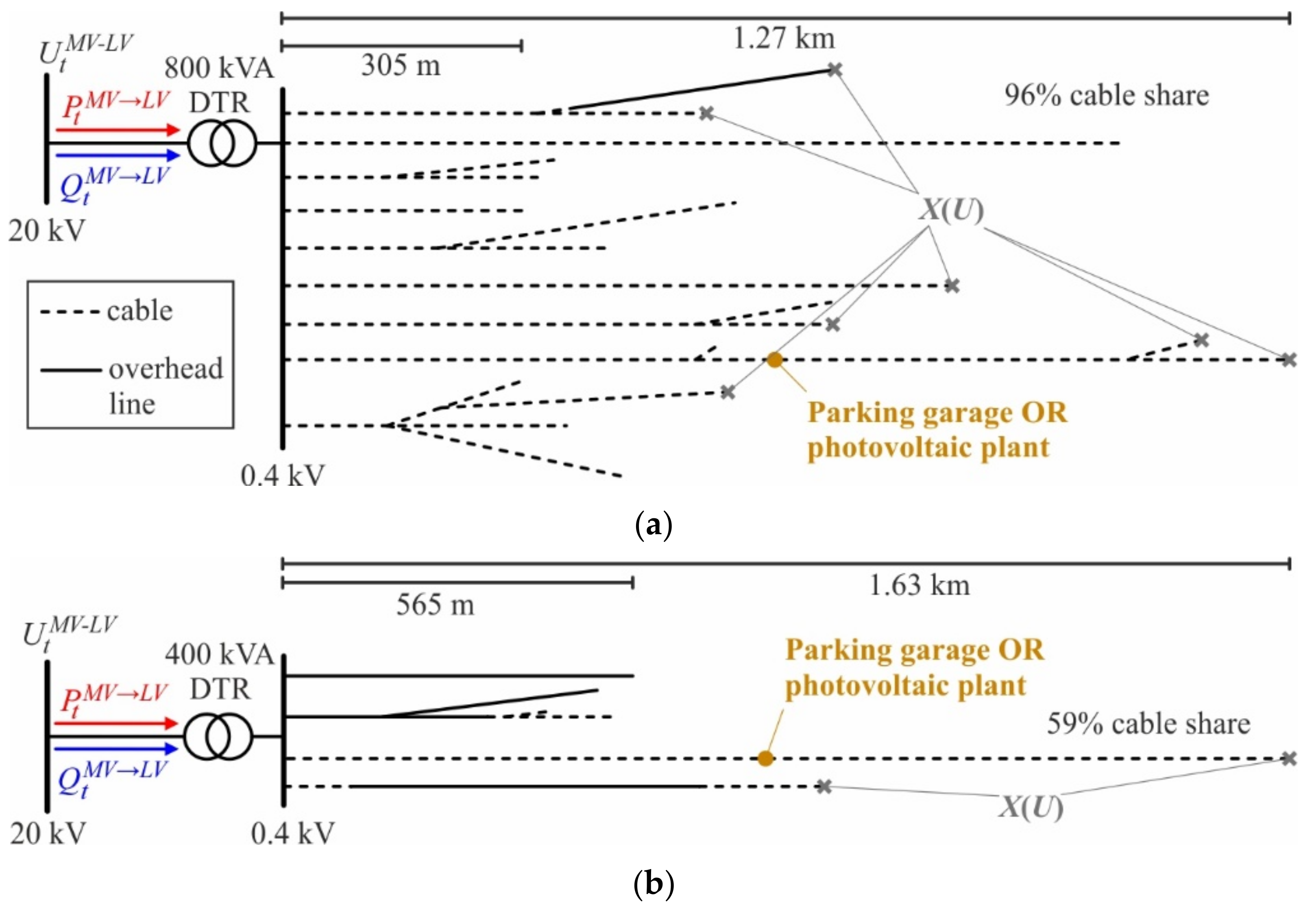
3.2.3. Low Voltage Grids

Figure 13 shows simplified one-line diagrams of two real Austrian LV grids; their exact model data is published in [37]. Grey crosses highlight the connection points of RPDs when X(U) or X(U)⁺ local control is used (see Section 3.1.2 and Section 3.1.3). Both grids are simulated for two different bulk loads connected at the position marked by the orange dot: parking garage (bulk consumer) and PV plant (bulk producer). The simulations are repeated for two distinct voltage values at the primary bus of the DTR: 0.95 and 1.05 p.u.

The urban LV grid shown in Figure 13a is connected to the medium-voltage grid through a 20 kV/0.4 kV DTR rated by 800 kVA (instead of the 630 kVA transformer documented in the data repository, a 800 kVA one is used due to the high DER penetration), whose tap changer is fixed in its mid-position. It includes nine feeders with a total line length of 12.82 km and a cable share of around 96% (the cable share is calculated by dividing the total length of all cables by the sum of the total lengths of all cables and overhead lines). The longest and shortest feeders are 1.27 km and 305 m long. They connect 88 residential prosumers and 87 residential consumers that are homogeneously distributed.

The rural LV grid shown in Figure 13b includes four feeders with an average cable share of around 59%. Its DTR is rated by 400 kVA (instead of the 160 kVA transformer documented in the data repository, a 400 kVA one is used due to the high DER penetration) and transforms 20 kV at the primary bus into 0.4 kV at the secondary one; the tap changer is fixed in mid-position. The shortest and longest feeder reach 565 m and 1.63 km, respectively. This LV grid connects homogeneously distributed residential prosumers (31) and consumers (30).

3.3. Overview of Scenarios

The control arrangements are simulated for both LV grids, bulk load setups, and two different DTR primary voltages: 0.95 and 1.05 p.u.

Table 1. Overview of the scenarios simulated for each control arrangement.

LV Grid	Bulk Load Setup	DTR Primary Voltage
Rural	Bulk consumer	0.95 p.u.
		1.05 p.u.
	Bulk producer	0.95 p.u.
		1.05 p.u.
Urban	Bulk consumer	0.95 p.u.
		1.05 p.u.
	Bulk producer	0.95 p.u.
		1.05 p.u.

overviews the scenarios simulated for each control arrangement described in Section 3.1.

3.4. Calculation Software and Algorithm

The models are implemented in the simulation software PSS^®®SINCAL (version 17.5) [38] and the Newton Raphson method is used to solve the load flow problem.

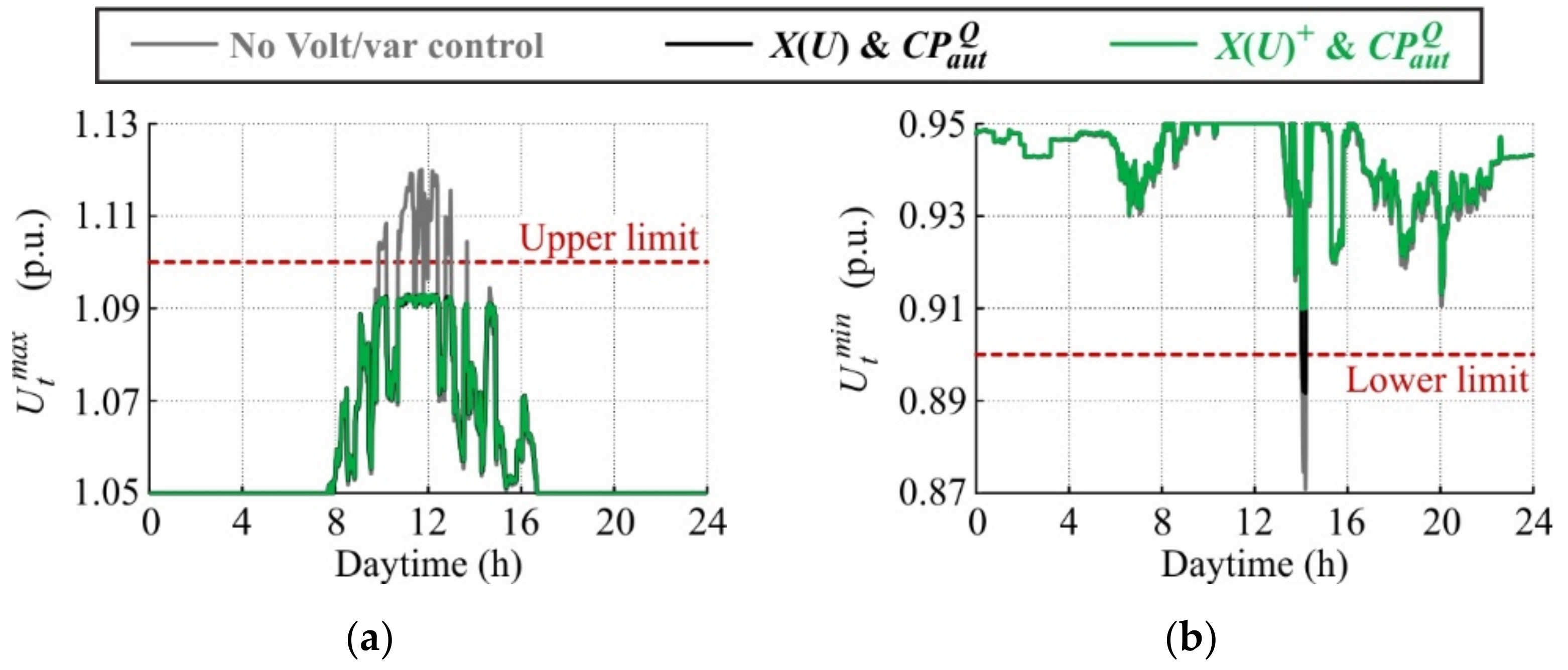
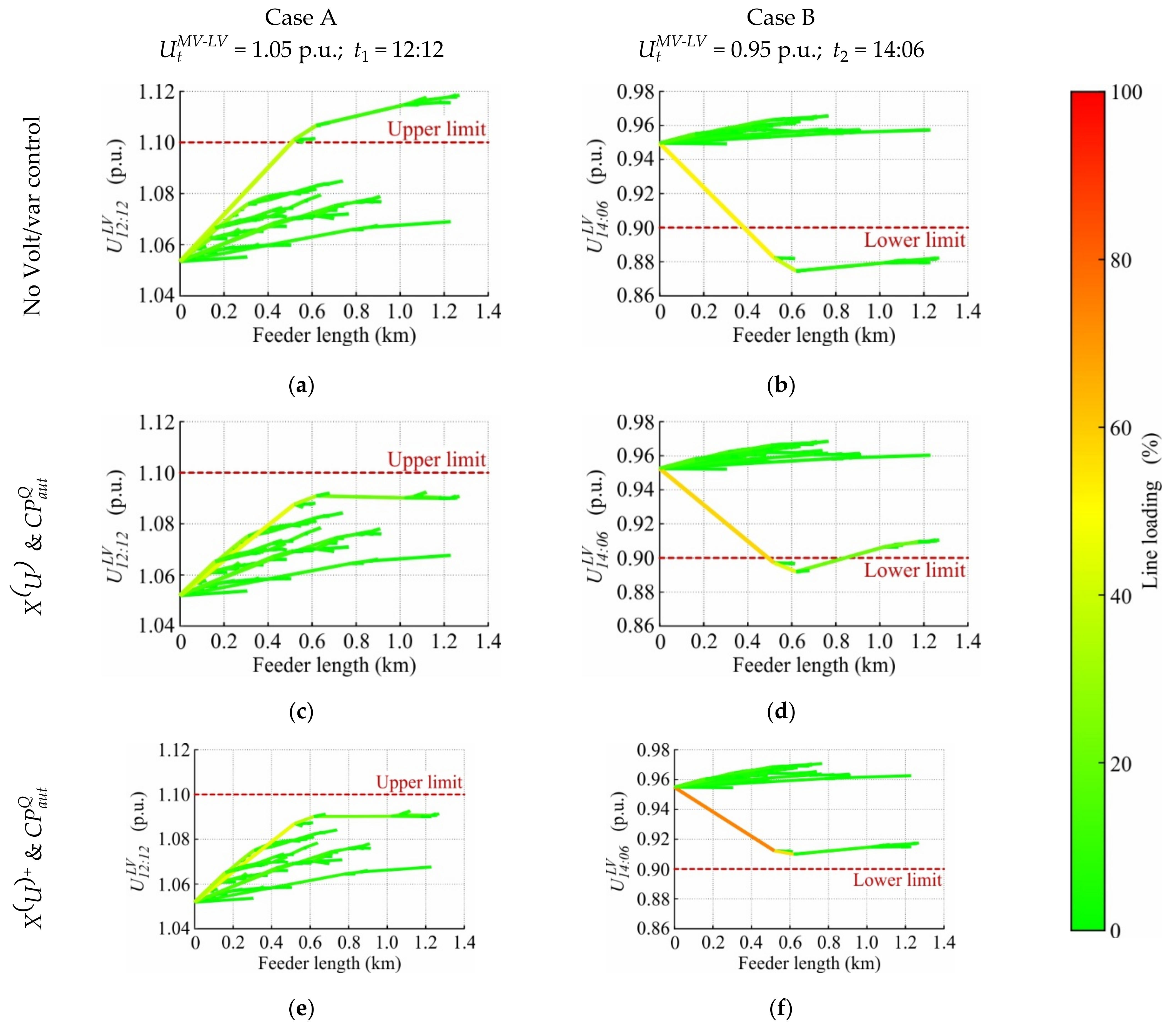
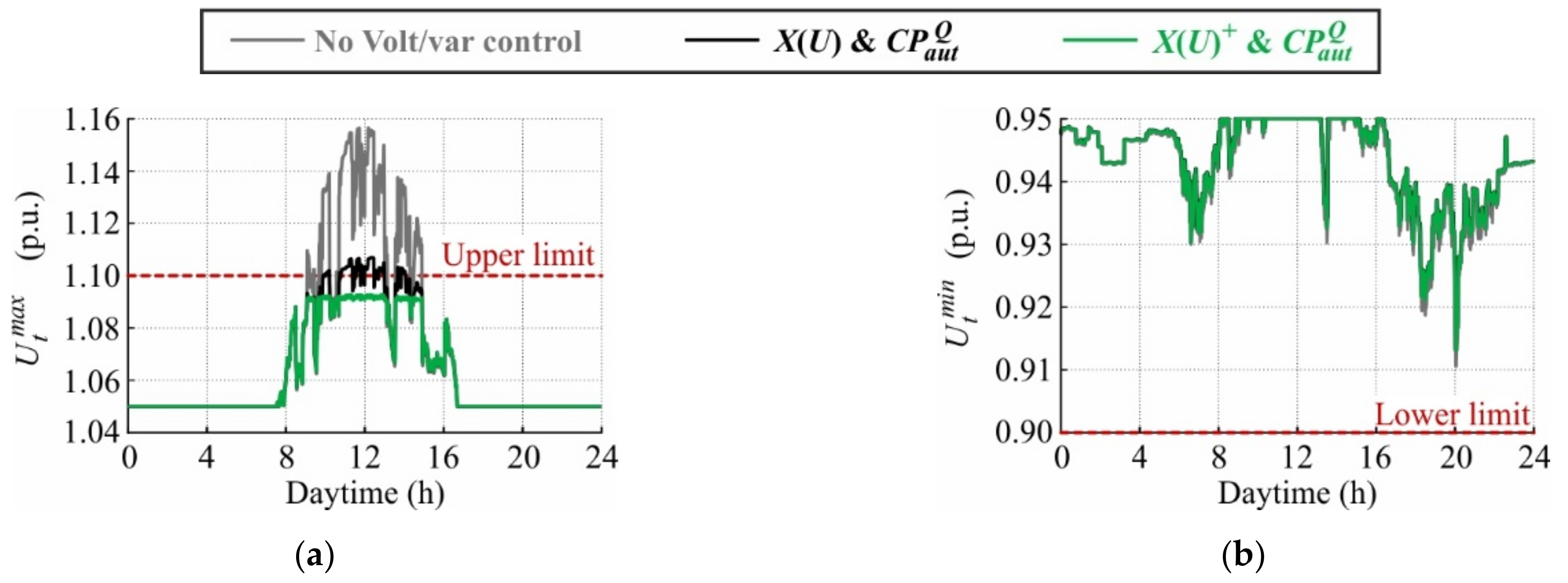
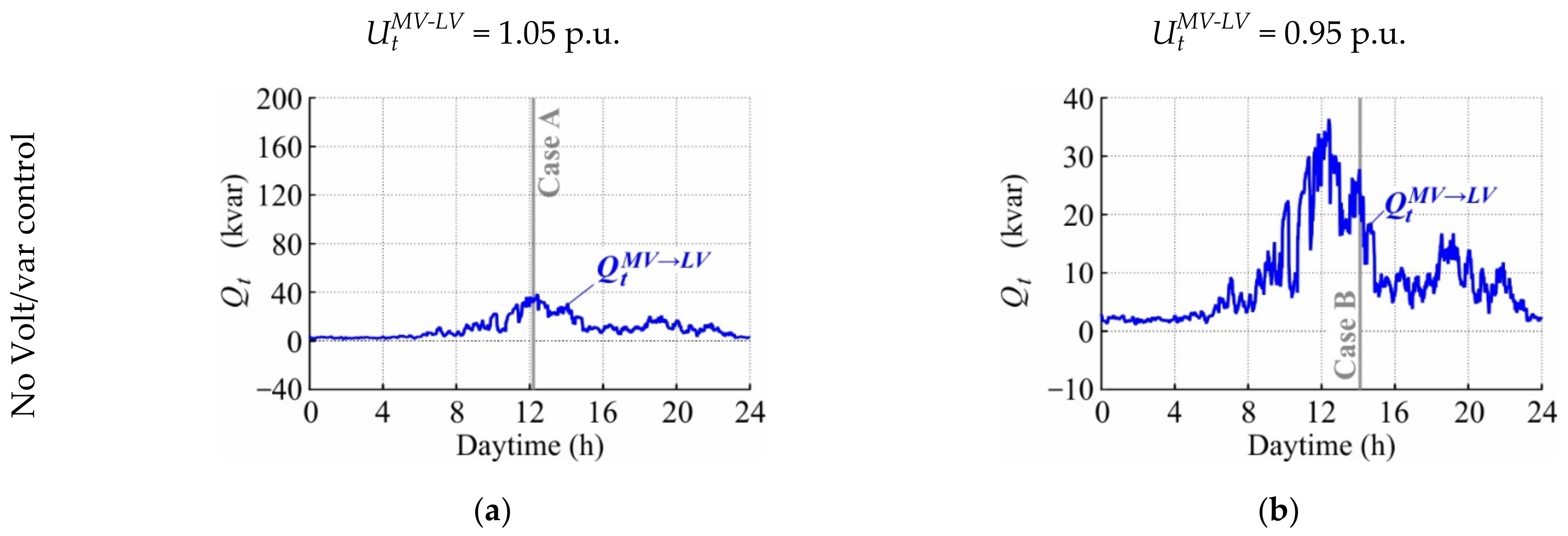
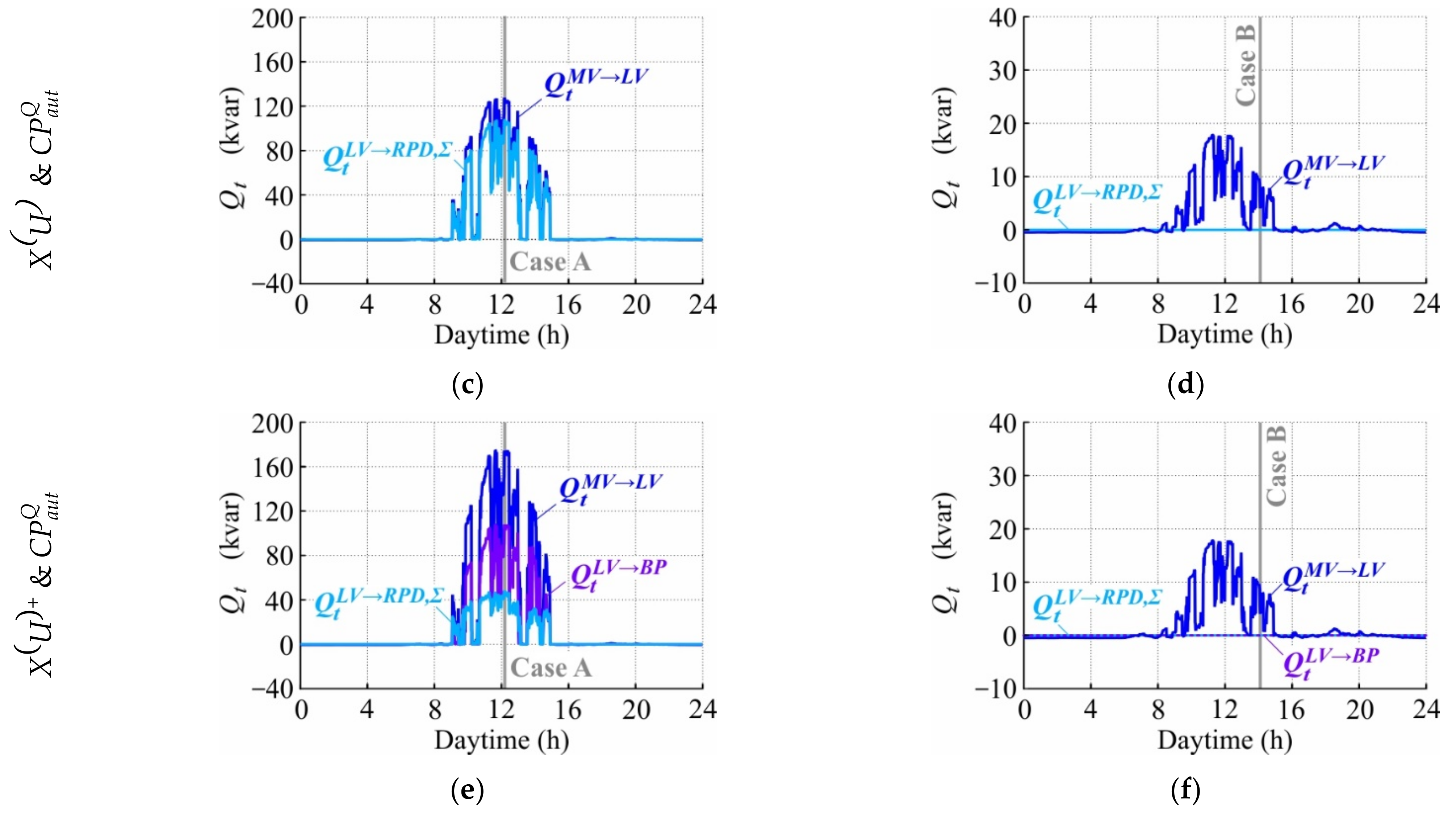
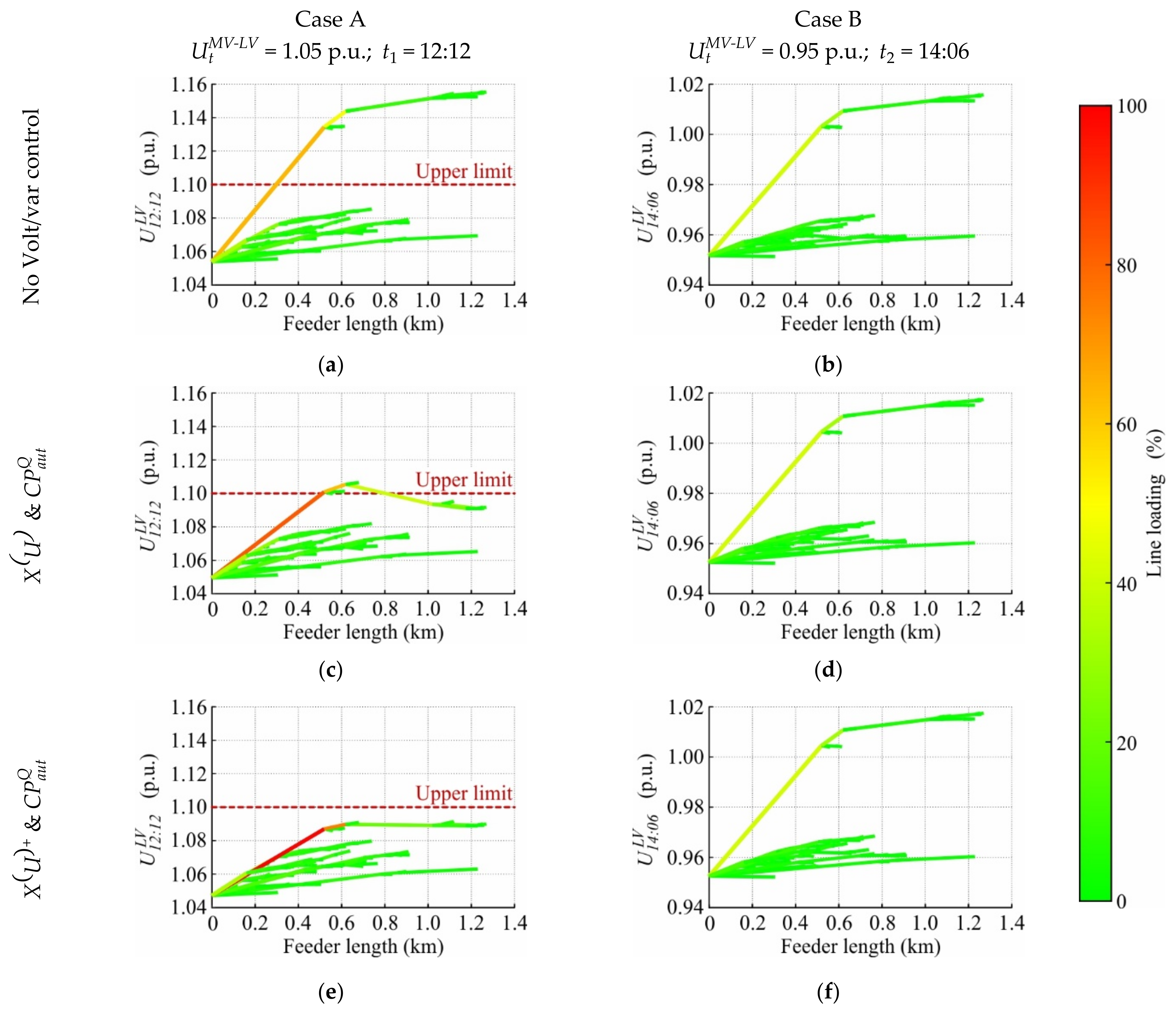
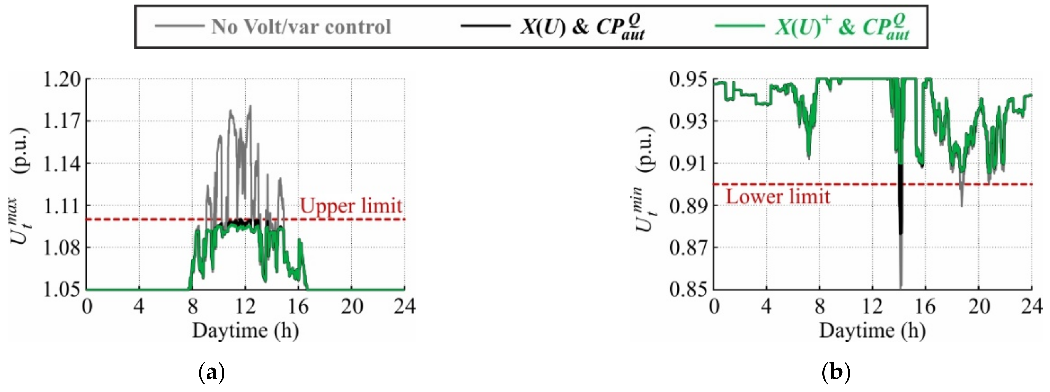
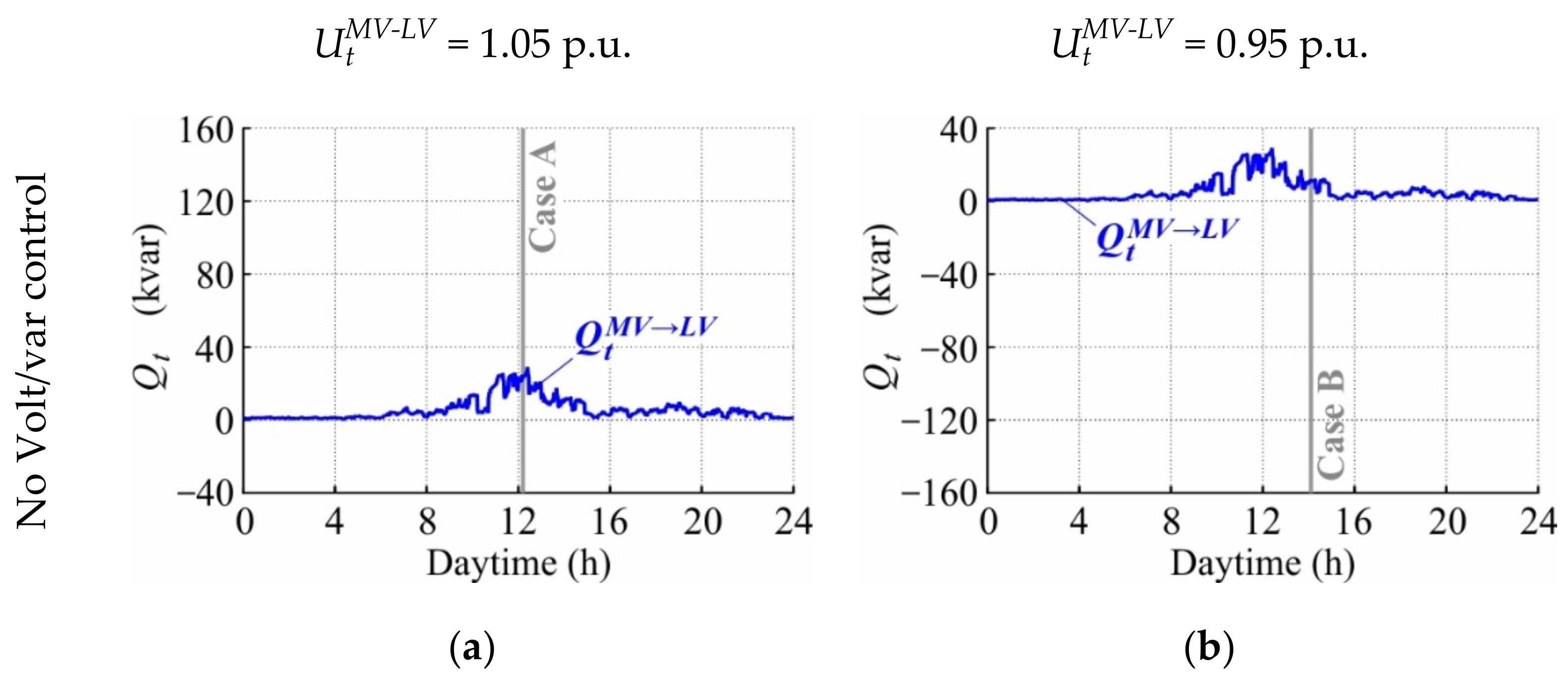
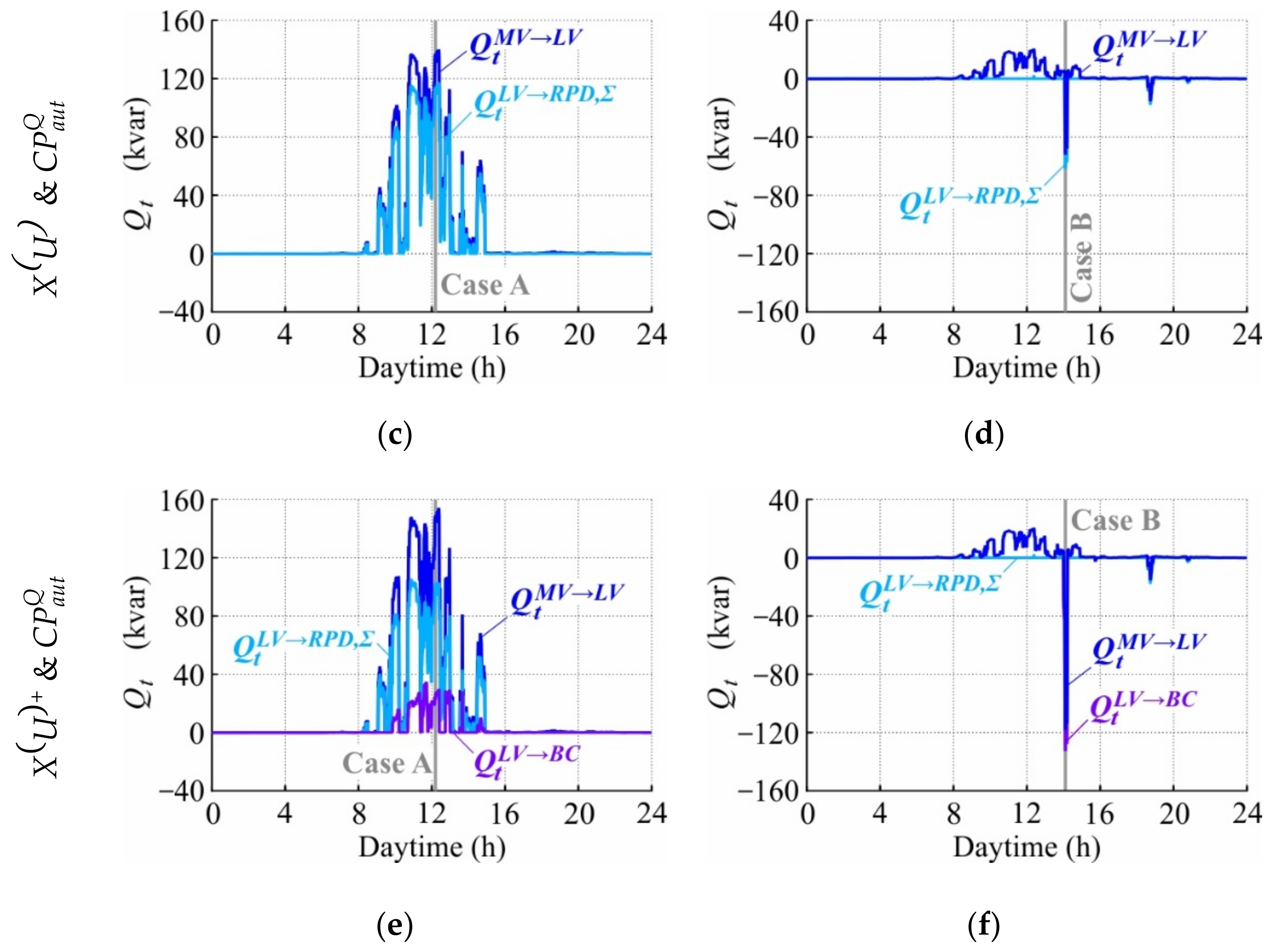
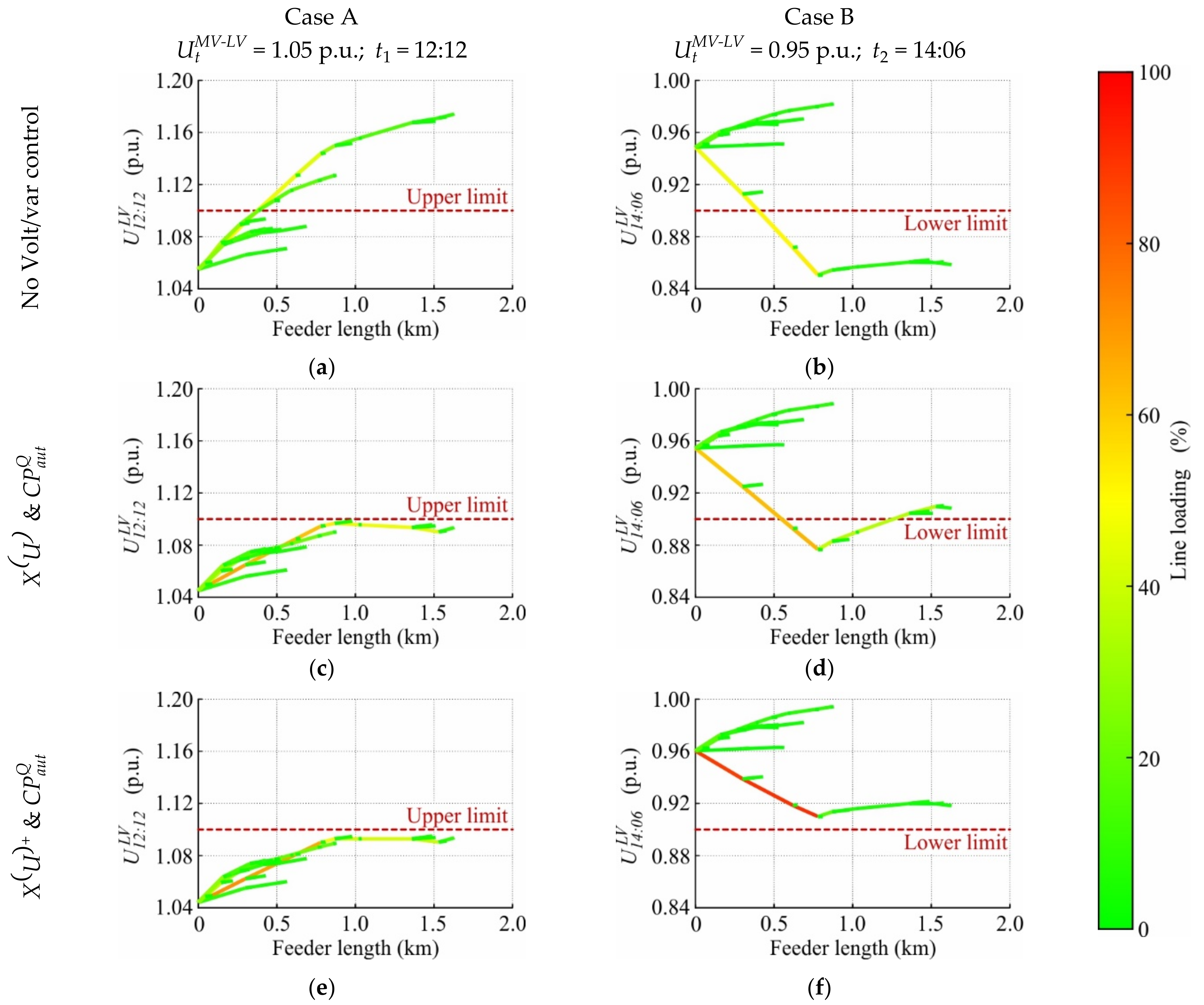
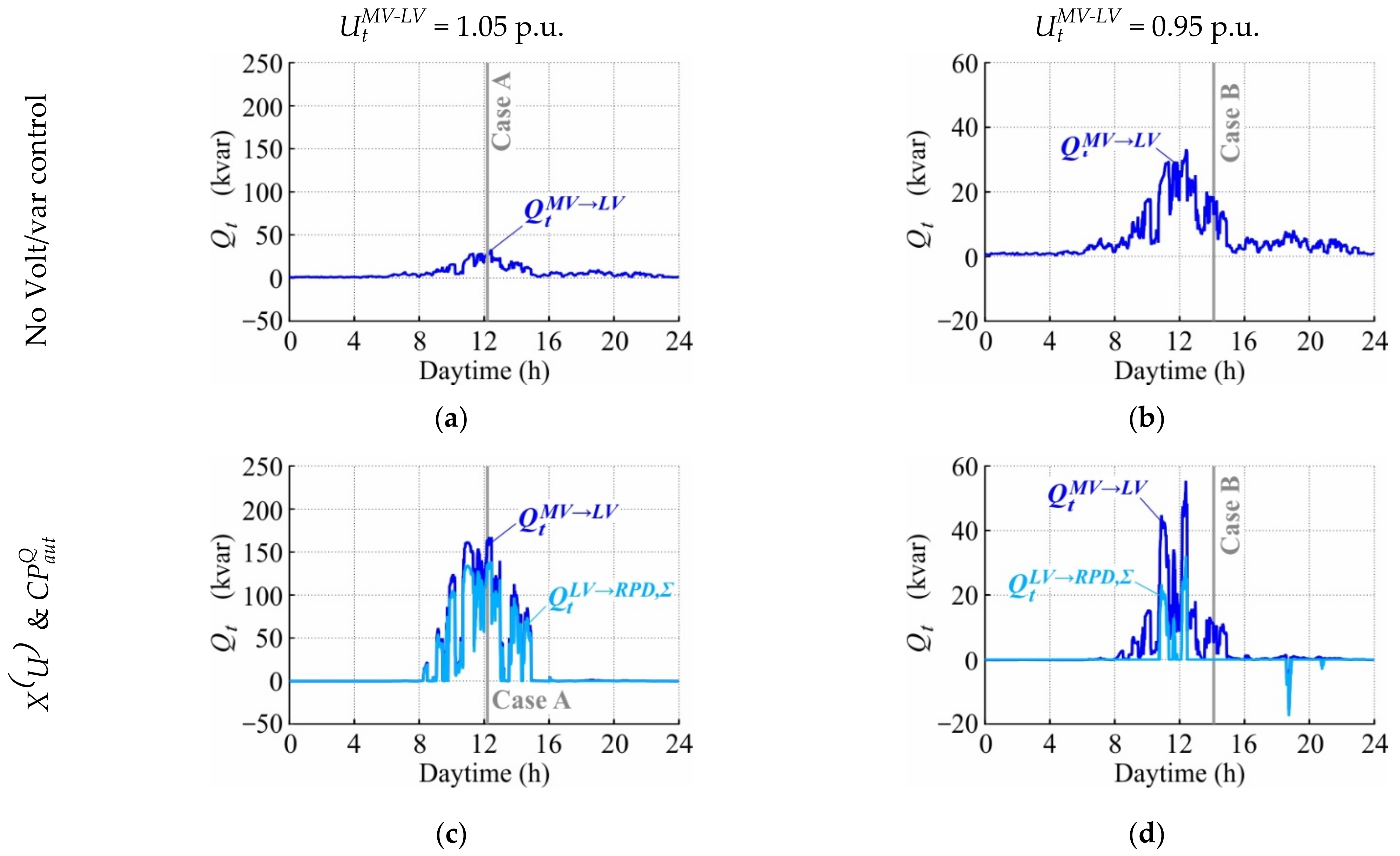
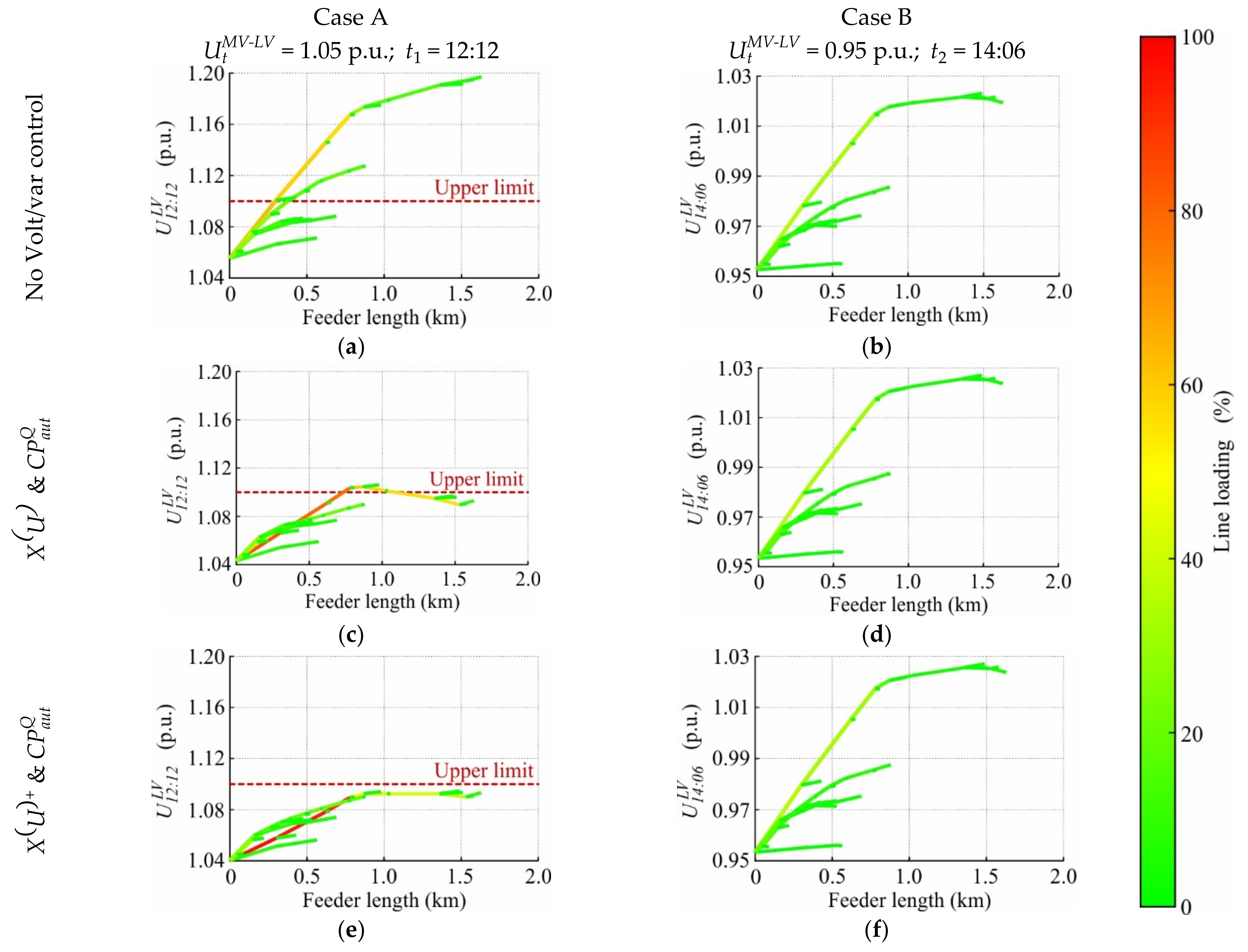
4. Volt/var Behavior of Low Voltage Grids

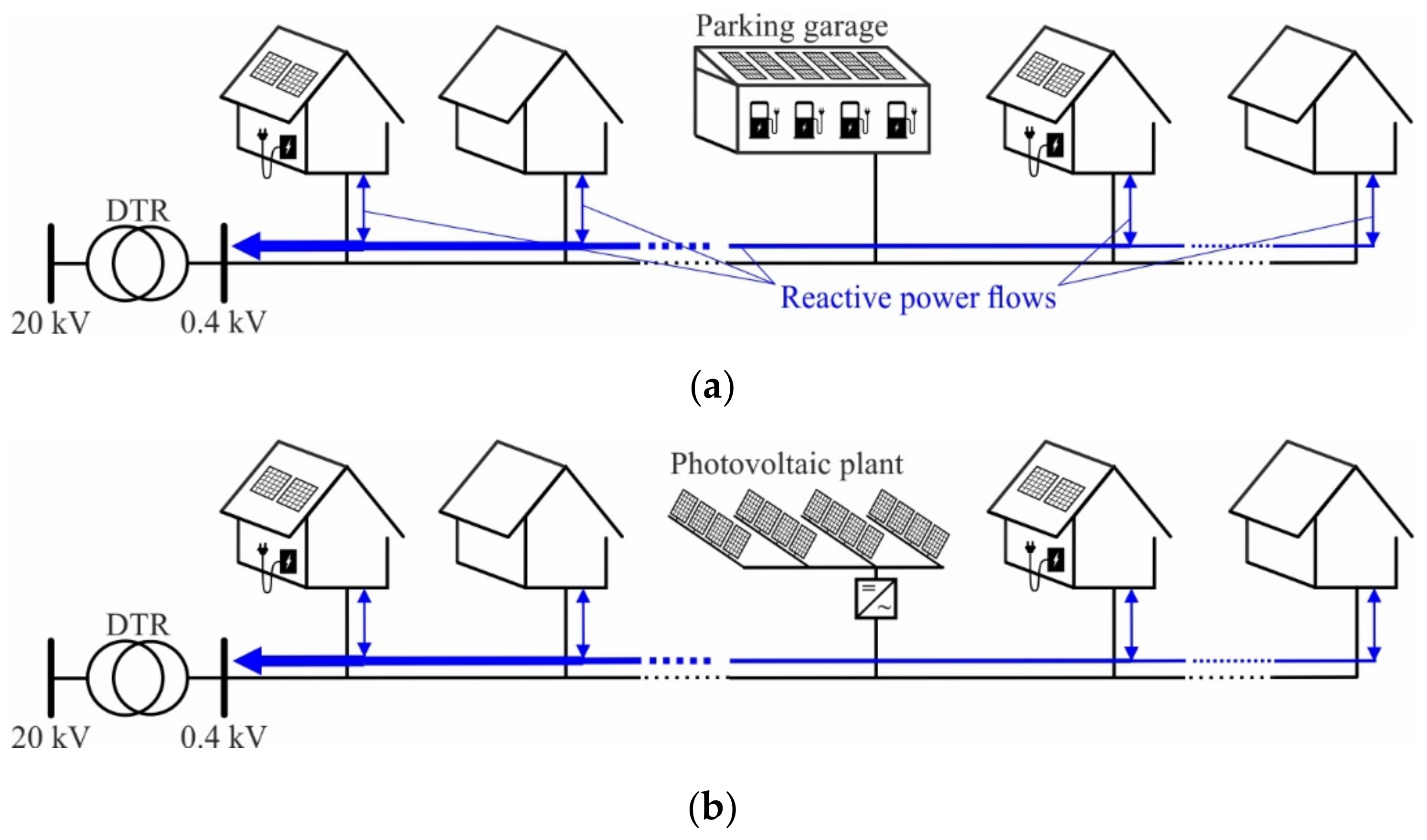
The steady-state behavior of both LV grids is discussed for the scenarios listed in Table 1. Voltage limit compliance is analyzed based on the maximal ($U_t^{max}$) and minimal ($U_t^{min}$) voltages of all LV nodes for each value of t. Furthermore, three different Q-contributions are analyzed:

• The MV→LV reactive power exchange ($Q_t^{MV\to LV}$);
• The reactive power contribution of the bulk consumer or producer ($Q_t^{LV\to BC}$ or $Q_t^{LV\to BP}$)
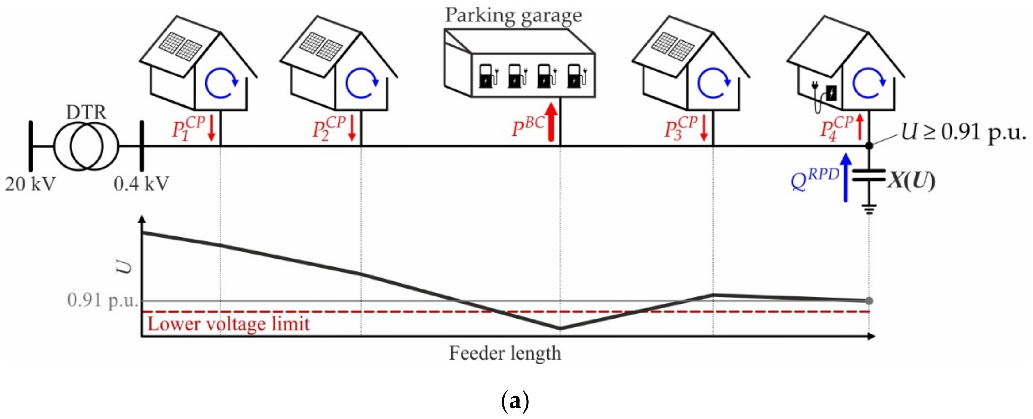
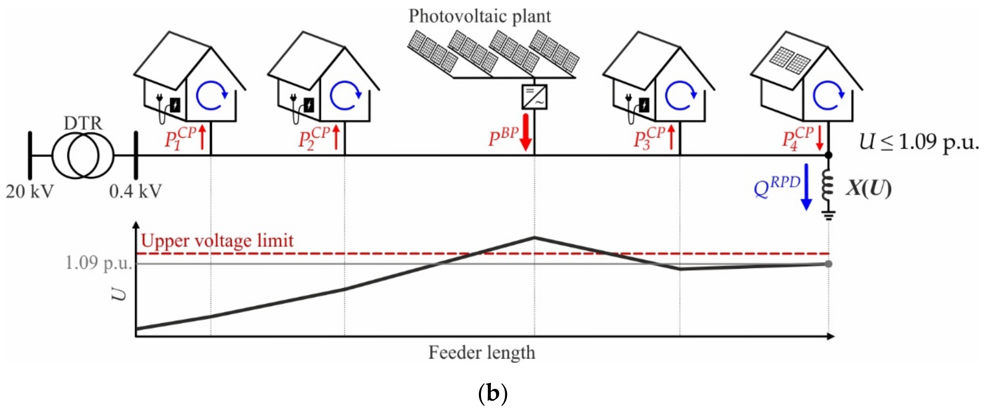
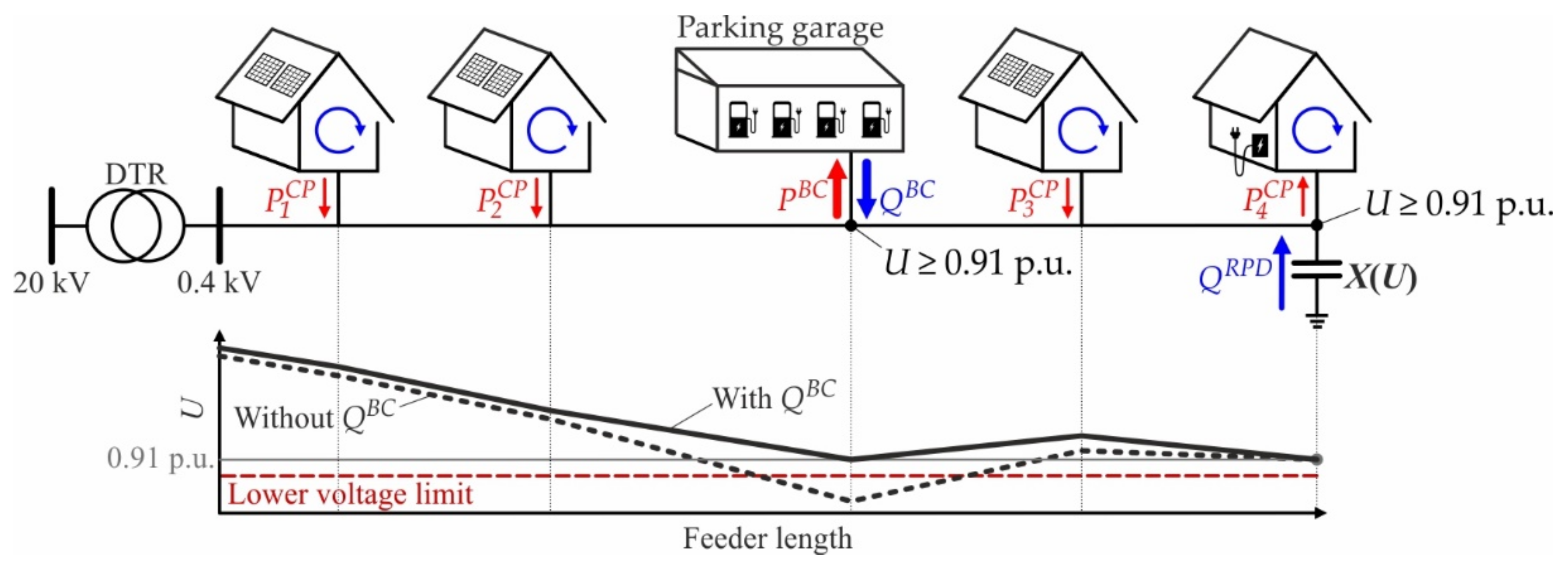
• The total reactive power contribution of all RPDs connected at the LV feeder ends ($Q_t^{LV\to RPD,\Sigma }$), calculated according to Equation (8).

  $$Q_t^{LV\to RPD,\Sigma }={{\displaystyle \sum }}_{\forall f}{Q}_{f,t}^{LV\to RPD}.$$

  (8)

  where $Q_{f,t}^{LV\to RPD}$ is the reactive power flowing from the LV grid into the RPD connected at the feeder end f at daytime t. Furthermore, the LV grid state, including voltage profiles and equipment loadings, is discussed for two critical cases that provoke high and low voltages at the LV level:
• Case A threatens the upper voltage limit due to high active power production $\left(t_1=12:12\right)$ and high DTR primary voltage $\left(U_t^{MV-LV}=1.05 \mathrm{p}.\mathrm{u}.\right)$.
• Case B threatens the lower voltage limit due to high active power consumption $\left(t_2=14:06\right)$ and low DTR primary voltage $\left(U_t^{MV-LV}=0.95 \mathrm{p}.\mathrm{u}.\right)$.

The equipment loading resulting in these cases is evaluated using the DTR ($Loadin{g}_t^{DTR}$) and maximum line segment loadings ($Loadin{g}_{max,t}^{line}$) along the feeders’ lengths.

The calculated reactive power and loading values are listed in

Table A1. Reactive power flows in different LV grids for different bulk load setups, control arrangements and cases.

LV Grid	Bulk Load Setup	Control Arrangement	Case	${\mathit{Q}}_{\mathit{t}}^{\mathit{M}\mathit{V}\to \mathit{L}\mathit{V}}$	${\mathit{Q}}_{\mathit{t}}^{\mathit{L}\mathit{V}\to \mathit{R}\mathit{P}\mathit{D},\mathit{\Sigma }}$	${\mathit{Q}}_{\mathit{t}}^{\mathit{L}\mathit{V}\to \mathit{B}\mathit{C}}$
				(kvar)	(kvar)	(kvar)
Urban	Bulk consumer	No VVC	A	27.127	0.000	0.000
			B	18.445	0.000	0.000
		$X\left(U\right) \& {\mathit{CP}}_{\mathit{aut}}^Q$	A	58.526	47.985	0.000
			B	−40.288	−44.760	0.000
		$X{\left(U\right)}^{+} \& {\mathit{CP}}_{\mathit{aut}}^Q$	A	61.094	43.464	7.095
			B	−88.373	0.000	−94.984
	Bulk producer	No VVC	A	32.214	0.000	0.000
			B	19.941	0.000	0.000
		$X\left(U\right) \& {\mathit{CP}}_{\mathit{aut}}^Q$	A	124.903	105.132	0.000
			B	4.025	0.000	0.000
		$X{\left(U\right)}^{+} \& {\mathit{CP}}_{\mathit{aut}}^Q$	A	172.767	47.388	103.538
			B	4.025	0.000	0.000
Rural	Bulk consumer	No VVC	A	23.150	0.000	0.000
			B	11.477	0.000	0.000
		$X\left(U\right) \& {\mathit{CP}}_{\mathit{aut}}^Q$	A	136.600	113.711	0.000
			B	−52.181	−61.215	0.000
		$X{\left(U\right)}^{+} \& {\mathit{CP}}_{\mathit{aut}}^Q$	A	148.222	102.300	22.546
			B	−118.448	0.000	−132.816
	Bulk producer	No VVC	A	26.487	0.000	0.000
			B	12.772	0.000	0.000
		$X\left(U\right) \& {\mathit{CP}}_{\mathit{aut}}^Q$	A	164.323	135.220	0.000
			B	5.058	0.000	0.000
		$X{\left(U\right)}^{+} \& {\mathit{CP}}_{\mathit{aut}}^Q$	A	198.305	98.718	68.306
			B	5.058	0.000	0.000

and

Table A2. Equipment loading in different LV grids for different bulk load setups, control arrangements and cases.

LV Grid	Bulk Load Setup	Control Arrangement	Case	$\mathit{L}\mathit{o}\mathit{a}\mathit{d}\mathit{i}\mathit{n}{\mathit{g}}_{\mathit{m}\mathit{a}\mathit{x},\mathit{t}}^{\mathit{l}\mathit{i}\mathit{n}\mathit{e}}$	$\mathit{L}\mathit{o}\mathit{a}\mathit{d}\mathit{i}\mathit{n}{\mathit{g}}_{\mathit{t}}^{\mathit{D}\mathit{T}\mathit{R}}$
				(%)	(%)
Urban	Bulk consumer	No VVC	A	38.05	45.31
			B	52.01	5.02
		$X\left(U\right) \& {\mathit{CP}}_{\mathit{aut}}^Q$	A	44.76	45.47
			B	57.85	6.64
		$X{\left(U\right)}^{+} \& {\mathit{CP}}_{\mathit{aut}}^Q$	A	45.50	45.51
			B	74.24	12.10
	Bulk producer	No VVC	A	64.21	51.53
			B	41.09	26.59
		$X\left(U\right) \& {\mathit{CP}}_{\mathit{aut}}^Q$	A	82.36	52.25
			B	41.01	26.47
		$X{\left(U\right)}^{+} \& {\mathit{CP}}_{\mathit{aut}}^Q$	A	99.14	53.60
			B	41.01	26.47
Rural	Bulk consumer	No VVC	A	51.01	66.33
			B	52.89	3.86
		$X\left(U\right) \& {\mathit{CP}}_{\mathit{aut}}^Q$	A	67.07	70.72
			B	64.75	14.61
		$X{\left(U\right)}^{+} \& {\mathit{CP}}_{\mathit{aut}}^Q$	A	71.38	71.89
			B	91.30	32.17
	Bulk producer	No VVC	A	63.41	72.23
			B	36.15	37.32
		$X\left(U\right) \& {\mathit{CP}}_{\mathit{aut}}^Q$	A	83.42	77.49
			B	35.95	37.20
		$X{\left(U\right)}^{+} \& {\mathit{CP}}_{\mathit{aut}}^Q$	A	97.12	81.14
			B	35.95	37.20

in Appendix B for the different Volt/var control arrangements and cases A and B.

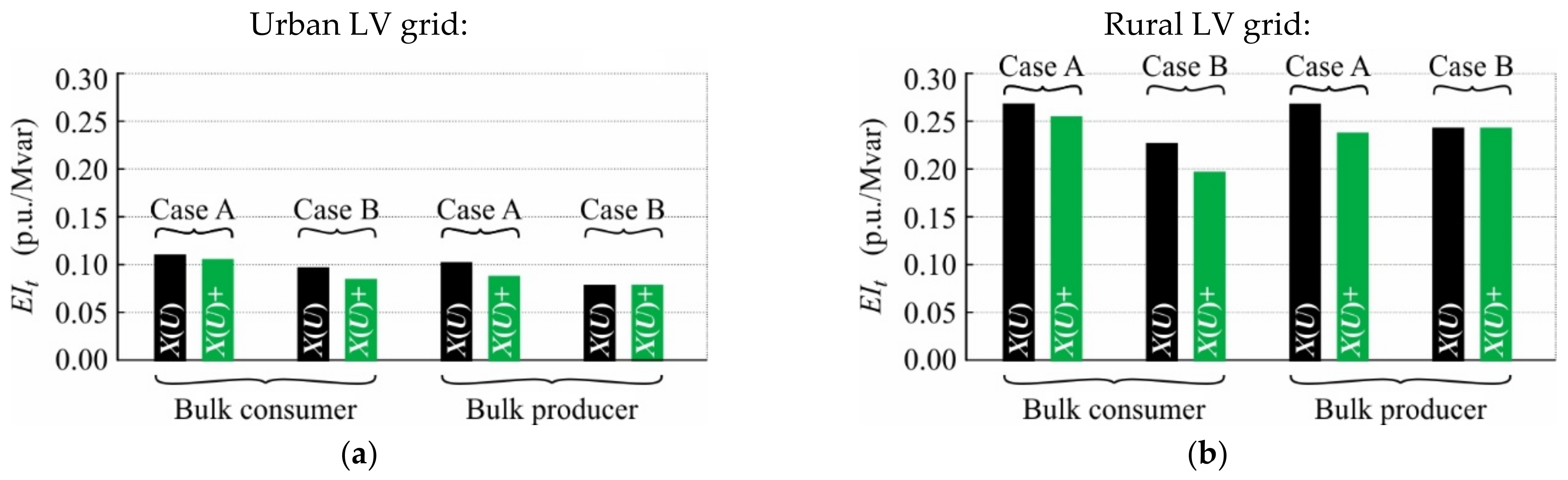
4.1. Urban Low Voltage Grid

4.1.1. With Bulk Consumer

Figure 14 shows the extrema of the urban LV grid’s node voltages in the presence of a bulk consumer for the investigated control arrangements. Most of the time, the arrangements including X(U) and X(U)⁺ local control behave similarly, so the corresponding curves overlap. Without any Volt/var control, the upper voltage limit is violated many times between 9:52 a.m. and 13:40 p.m. (see Figure 14a). These limit violations are eliminated throughout the entire time horizon when X(U) or X(U)⁺ local control are combined with Q-Autarkic CPs. However, Figure 14b shows that the former combination does not prevent lower limit violations in times of bulk consumption, i.e., around 14:09 p.m.

Figure 15 shows the daily reactive power flows within the urban LV grid with a bulk consumer for different DTR primary voltages and control arrangements. Without any Volt/var control, no RPDs are connected, and the bulk consumer does not contribute any reactive power. Figure 15a,b show that 27.13 and 18.45 kvar flow from the MV into the LV level in cases A and B, respectively. The arrangement with X(U) local control and CP_Q-Autarky modifies the MV→LV reactive power exchange fundamentally: The Q-exchange is determined exclusively by the grid losses and the behavior of RPDs. In Figure 15c, almost no reactive power is exchanged before 9:44 and after 14:39, while in between, high Q-amounts flow into the LV grid to cover the RPDs’ absorption. In case A, the X(U)-controlled RPDs absorb 47.99 kvar in total, leading to an MV→LV reactive power flow of 58.53 kvar. Figure 15d shows that the RPDs inject reactive power between 14:01 p.m. and 14:12 p.m., i.e., during periods of excessive EV charging, reaching—in total—44.76 kvar in case B. Consequently, 40.29 kvar flow from the LV into the MV level. The bulk consumer provides reactive power when X(U)⁺ local control is used, reducing the RPDs’ total reactive power contribution while increasing the MV→LV reactive power exchanges. In Figure 15e, the bulk consumer absorbs relatively low amounts of reactive power around midday: In case A, 7.10 and 43.46 kvar are drawn by the parking garage and RPDs, respectively, and 61.09 kvar flow from the MV into the LV level. Meanwhile, as shown in Figure 15f for case B, the parking garage injects 94.98 kvar; thus, 88.37 kvar flows from the LV into the MV grid. Here, the RPDs located at the feeder ends do not contribute any reactive power.

Figure 16 shows the grid state diagrams of the urban LV grid with a bulk consumer for different cases and control arrangements. Voltage limit violations occur in the whole rear part of the critical feeder when no Volt/var control is used. In Figure 16a, the upper limit is violated from a feeder length of 0.51 km, and DTR and maximum line segment loadings of 45.31 and 38.05% prevail. Meanwhile, in Figure 16b, the lower limit is violated from a distance of 0.38 km. The DTR loading reaches 5.02%, and the maximal line segment loading amounts to 52.01%. Figure 16c shows that the application of X(U) local control and CP_Q-Autarky successfully eliminates all upper limit violations by increasing the DTR and maximum line segment loadings to 45.47 and 44.76%, respectively. However, this control arrangement cannot remove the lower limit violations in the middle part (from 0.49 to 0.84 km feeder length) of the critical feeder when a bulk consumer is connected in this region (see Figure 16d). Here, the DTR is loaded by 6.64%, and a maximum line segment loading of 57.85% occurs. As shown in Figure 16e,f, the X(U)⁺ local control combined with CP_Q-Autarky eliminates all limit violations by increasing the line and DTR loadings. Case A provokes DTR and maximum line segment loadings of 45.51 and 45.50%, and in case B, they reach 12.10 and 74.24%.

4.1.2. With Bulk Producer

Figure 17 shows the extrema of the urban LV grid’s node voltages in the presence of a bulk producer for the investigated control arrangements. Similar to the setup with a bulk consumer, the curves of the different control arrangements overlap many hours a day. Figure 17a shows excessive upper limit violations between 9:05 a.m. and 14:53 p.m. when no Volt/var control is used. In contrast to X(U)⁺ local control, the X(U) strategy cannot eliminate all of these limit violations. Meanwhile, the lower limit is not violated, even without any Volt/var control; see Figure 17b.

Figure 18 shows the daily reactive power flows within the urban LV grid with a bulk producer for different DTR primary voltages and control arrangements. Figure 18a,b shows that 32.21 and 19.94 kvar flow from the MV into the LV level in cases A and B, respectively, when no Volt/var control is applied. For a DTR primary voltage of 1.05 p.u., the combination of X(U) local control with CP_Q-Autarky almost eliminates the reactive power flows through the distribution substation before 9:04 and after 14:54 (see Figure 18c). In between, the RPDs connected at the feeder ends consume reactive power, and the active power injection of PVs provokes significant reactive power losses within the LV lines and DTR. In case A, the RPDs absorb 105.13 kvar in total, causing an MV→LV reactive power flow of 124.90 kvar. Figure 18d shows that the X(U) local controls remain inactive for a DTR primary voltage of 0.95 p.u., leading to very low reactive power exchanges between the MV and LV levels: 4.03 kvar flow from the MV into the LV grid in case B. The highest reactive power flows occur when the ‘$X{\left(U\right)}^{+} \& {\mathit{CP}}_{\mathit{aut}}^Q$’ control arrangement is applied. The significant Q-absorption of the bulk producer shown in Figure 18e reduces the total reactive power contribution of RPDs but increases the MV→LV flow. In case A, the bulk producer consumes 103.54 kvar, the RPDs consume 47.39 kvar in total and 172.77 kvar flow from the MV into the LV grid. Due to the inactivity of X(U)⁺ control for a DTR primary voltage of 0.95 p.u., the same results are obtained as for the ‘$X\left(U\right) \& {\mathit{CP}}_{\mathit{aut}}^Q$’ control arrangement (see Figure 18f).

Figure 19 shows the grid state diagrams of the urban LV grid with a bulk producer for different cases and control arrangements. Without any Volt/var control, the upper limit is violated from a feeder length of 0.30 km in Case A, and the DTR and maximal line segment loadings amount to 51.53 and 64.21%, respectively (see Figure 19a). Figure 19b shows that all node voltages lie within the acceptable range in case B, and the line segment loading reaches a maximum value of 41.09%. Here, the DTR is loaded by 26.59%. The combination of X(U) local control and CP_Q-Autarky does not maintain acceptable voltages throughout the entire feeder length: As illustrated in Figure 19c, the upper limit is violated between 0.51 and 0.80 km in case A, and the DTR and maximum line segment loadings are increased to 52.25 and 82.36%. The arrangement including X(U)⁺ local control eliminates all upper limit violations and provokes a DTR loading of 53.60% and a maximum line segment loading of 99.14% in case A (see Figure 19e). Figure 19d,f show that Q-Autarkic CPs slightly increase the voltages in case B while decreasing the DTR and maximum line segment loadings to 26.47 and 41.01%.

4.2. Rural Low Voltage Grid

4.2.1. With Bulk Consumer

Figure 20 shows the extrema of the rural LV grid’s node voltages in the presence of a bulk consumer for the investigated control arrangements. The results resemble the ones of the urban LV grid shown in Figure 14. In Figure 20a, numerous violations of the upper voltage limit occur between 9:05 a.m. and 14:53 p.m. when no Volt/var control is applied. Both investigated control strategies successfully remove these limit violations. However, Figure 20b shows that only the ‘$X{\left(U\right)}^{+} \& {\mathit{CP}}_{\mathit{aut}}^Q$’ control arrangement eliminates all violations of the lower voltage limit, which occur around 14:09 p.m. when no Volt/var control is used.

Figure 21 shows the daily reactive power flows within the rural LV grid with a bulk consumer for different DTR primary voltages and control arrangements. The MV-LV reactive power exchange without any Volt/var control is determined solely by the Q-contribution of the residential CPs and the Q-losses within the LV grid. A total of 23.15 kvar flow from the MV into the LV grid in case A (see Figure 21a), while in case B, the flow amounts to 11.48 kvar (see Figure 21b). In Figure 21c, very low Q-amounts flow through the distribution substation before 8:12 a.m. and after 14:54 p.m. In between, the RPDs’ high absorption drastically increases the MV→LV reactive power flows: In case A, the RPDs consume 113.71 kvar in total, provoking 136.60 kvar at the distribution substation level. For a DTR primary voltage of 0.95 p.u., the X(U) local control is inactive most of the time, except for a short period around 14:09 p.m. (see Figure 21d). In case B, the RPDs’ total injection of 61.22 kvar leads to an LV→MV reactive power flow of 52.18 kvar. In Figure 21e, the Q-absorption of the bulk consumer decreases the RPDs’ total consumption but increases the reactive power flows at the MV-LV boundary: In case A, the bulk consumer’s absorption of 22.55 kvar reduces the RPDs’ total consumption to 102.30 kvar and increases the MV→LV reactive power flow to 148.22 kvar. Figure 21f shows that the RPDs do not contribute any reactive power in case B. Voltage is maintained by the bulk consumer’s injection, which amounts to 132.82 kvar and provokes an LV→MV flow of 118.45 kvar.

Figure 22 shows the grid state diagrams of the rural LV grid with a bulk consumer for different cases and control arrangements. Without any Volt/var control, the upper and lower voltage limits are violated from feeder lengths of 0.38 and 0.40 km (see Figure 22a,b). In case A, DTR and maximum line segment loadings of 66.33 and 51.01% prevail, while in case B, these loading values amount to 3.86 and 52.89%. Figure 22c,d show that combining X(U) local control with CP_Q-Autarky eliminates the upper but not the lower voltage limit violations: the lower one is violated from 0.55 to 1.26 km feeder length. In case A, the DTR and maximum line segment loadings amount to 70.72 and 67.07%, while in case B, they reach 14.61 and 64.75%. The ‘$X{\left(U\right)}^{+} \& {\mathit{CP}}_{\mathit{aut}}^Q$’ control arrangement successfully eliminates all voltage limit violations while increasing the DTR and maximum line segment loadings to 71.89 and 71.38% in case A (see Figure 22e), and to 32.17 and 91.30% in case B (see Figure 22f).

4.2.2. With Bulk Producer

Figure 23 shows the extrema of the rural LV grid’s node voltages in the presence of a bulk producer for the investigated control arrangements. The upper voltage limit is violated several times between 8:18 and 14:54 when no Volt/var control is used, and between 9:52 a.m. and 14:42 p.m. when X(U) local control is combined with CP_Q-Autarky (see Figure 23a). Meanwhile, all upper limit violations are eliminated by the ‘$X{\left(U\right)}^{+} \& {\mathit{CP}}_{\mathit{aut}}^Q$’ control arrangement. Figure 23b shows that without any Volt/var control, the lower voltage limit is violated around 18:44 p.m. Both control arrangements successfully eliminate these violations.

Figure 24 shows the daily reactive power flows within the rural LV grid with a bulk producer for different DTR primary voltages and control arrangements. In Figure 24a,b, where no Volt/var control is applied, reactive power flows from the MV into the LV grid, reaching 26.49 and 12.77 kvar in cases A and B, respectively. The reactive power flows are drastically increased when Volt/var control is used. In Figure 24c, large Q-amounts are contributed in total by the RPDs (135.22 kvar in case A), provoking excessive reactive power flows at the MV-LV boundary (164.32 kvar in case A). For a DTR primary voltage of 0.95 p.u., the RPDs’ total Q-contribution is characterized by four significant peaks around 11:00 a.m., 11:40 a.m., 12:20 p.m., and 18:44 p.m. (see Figure 24d). However, they do not contribute any reactive power in case B. Here, the Q-Autarky of CPs reduces the MV→LV flow, reaching 5.06 kvar in case B. In analogy with the results presented for the urban LV grid (see Figure 18e), the total Q-contribution of the RPDs is reduced and the flow at the distribution substation level is increased by the reactive power consumption of the bulk producer. In case A, the bulk producer draws 68.31 kvar from the grid, and the RPDs absorb 98.72 kvar in total, provoking an MV→LV flow of 198.30 kvar. The bulk producer does not contribute any reactive power for a DTR primary voltage of 0.95 p.u. Therefore, the same results are shown in Figure 24f as in Figure 24d.

Figure 25 shows the grid state diagrams of the rural LV grid with a bulk producer for different cases and control arrangements. In Figure 25a, where no Volt/var control is applied, upper voltage limit violations appear from a feeder length of 0.3 km. The DTR is loaded by 72.23% and the maximal line segment loading amounts to 63.41%. Meanwhile, as Figure 25b shows, no limit violations occur in case B, and the DTR and maximum line segment loadings reach 37.32 and 36.15%. The combination of X(U) local control with CP_Q-Autarky does not eliminate all limit violations: the upper limit is exceeded from 0.73 to 1.09 km of feeder length in case A (see Figure 25c). This control arrangement increases the DTR and maximum line segment loadings to 77.49 and 83.42%. The RPDs are inactive in case B (see Table A1), so the CP_Q-Autarky reduces the DTR and maximum line segment loadings to 37.20 and 35.95%, respectively (see Figure 25d). Meanwhile, the ‘$X{\left(U\right)}^{+} \& {\mathit{CP}}_{\mathit{aut}}^Q$’ control arrangement prevents violations of the voltage limits. In case A (see Figure 25e), the DTR and maximum line segment loadings reach 81.14 and 97.12%, while in case B (see Figure 25f), the same results are obtained as for the ‘$X\left(U\right) \& {\mathit{CP}}_{\mathit{aut}}^Q$’ control arrangement.

5. Discussion

The analysis presented in Section 4 showed that the X(U) local control strategy combined with Q-Autarkic CPs does not eliminate all voltage limit violations when bulk loads are present. The non-monotonous voltage profiles may violate the limits somewhere along the LV feeders although the voltages at the feeders’ ends remain within the acceptable range.

Furthermore, it shows that the introduced extension of the X(U) local control arrangement successfully eliminates all voltage limit violations while decreasing the necessary rating of the RPDs connected at the feeders’ ends. However, involving the bulk loads in Volt/var control provokes distributed var contributions, contradicting the idea of maximal control effectiveness presented in Section 2.2. Increased reactive power flows and equipment loading within the LV grid are the consequence. The effectiveness index ($E{I}_t$) is defined in Equation (9) to assess the effectiveness of the original and extended control arrangements based on the simulation results. A high index indicates a great effect of the reactive power on the voltages within the LV grid.

$$E{I}_t=-\frac{1}{N}·{{\displaystyle \sum }}_{n=1}^N\left(U_{n,t}^{VVC}-U_{n,t}^{noVVC}\right)/\left(Q_t^{MV\to LV,VVC}-Q_t^{MV\to LV,noVVC}\right).$$

(9)

where $N$ is the number of LV grid nodes; $U_{n,t}^{VVC}$ is the voltage of node $n$ when Volt/var control is used; $U_{n,t}^{noVVC}$ is the voltage of node $n$ when no Volt/var control is used; $Q_t^{MV\to LV,VVC}$ is the MV→LV reactive power flow when Volt/var control is used; and $Q_t^{MV\to LV,noVVC}$ is the MV→LV reactive power flow when no Volt/var control is used.

Figure 26 shows the effectiveness index for all investigated scenarios. On first glance, a higher effectiveness of both control arrangements is observable in the rural compared to the urban LV grid, which is due to its relatively long feeders (see Equation (7), X is large for long feeders). Furthermore, the ‘$X\left(U\right) \& {\mathit{CP}}_{\mathit{aut}}^Q$’ control arrangement is generally more effective than the ‘$X{\left(U\right)}^{+} \& {\mathit{CP}}_{\mathit{aut}}^Q$’ one, as it provokes purely concentrated var contributions. Only in case B of the bulk producer setup do both controls show the same effectiveness. Here, the bulk producer does not contribute any reactive power, so both arrangements behave equally.

PV plants and some electric vehicle chargers have the capability to provide reactive power. The X(U) control scheme can be implemented directly into these distributed energy resources instead of installing RPDs at their delivery points (as it is done in the models, see Figure 12a,c).

6. Conclusions

The simulation results reveal the inability of the X(U) local control to maintain acceptable voltages at the low voltage level when bulk loads, such as electric vehicle parking garages and community-owned photovoltaic plants, are connected close to the feeder middle. In the presence of bulk loads, prosumers, and consumers, the feeders’ voltage profiles may be non-monotonous, so limit violations may occur somewhere along the feeders although the X(U) local control keeps the voltages at the feeders’ ends within the permissible band. The introduced extended control arrangement resolves this issue by implementing the X(U) local control scheme not only at the feeders’ ends but also into the bulk loads. This solution maintains voltage limit compliance reliably but deteriorates the effectiveness of the original X(U) local control: reactive power flows and equipment loading within the low voltage grids are increased. However, involving bulk loads in X(U) local control reduces the necessary rating of the reactive power devices connected at the feeders’ ends.

References

1. Status of Power System Transformation 2019: Power System Flexibility—Analysis. Available online: https://www.iea.org/reports/status-of-power-system-transformation-2019 (accessed on 6 February 2022).
2. Global Energy Review 2020—Analysis. Available online: https://www.iea.org/reports/global-energy-review-2020 (accessed on 16 December 2021).
3. ENTSO-E. ENTSO-E Position Paper on “Electric Vehicle Integration into Power Grids”; NTSO-E: Brussels, Belgium, 2021. [Google Scholar]
4. Joint Research Centre (European Commission); Uihlein, A.; Caramizaru, A. Energy Communities: An Overview of Energy and Social Innovation; Publications Office of the European Union: Luxembourg, 2020; ISBN 978-92-76-10713-2. [Google Scholar]
5. European Committee of the Regions; Milieu Ltd.; O’Brien, S.; Monteiro, C.; Gancheva, M.; Crook, N. Models of Local Energy Ownership and the Role of Local Energy Communities in Energy Transition in Europe; Publications Office of the European Union: Luxembourg, 2018; ISBN 978-92-895-0989-3. [Google Scholar]
6. Lopes, J.A.P.; Hatziargyriou, N.; Mutale, J.; Djapic, P.; Jenkins, N. Integrating Distributed Generation into Electric Power Systems: A Review of Drivers, Challenges and Opportunities. Electr. Power Syst. Res. 2007, 77, 1189–1203. [Google Scholar] [CrossRef] [Green Version]
7. Manditereza, P.T.; Bansal, R. Renewable Distributed Generation: The Hidden Challenges—A Review from the Protection Perspective. Renew. Sustain. Energy Rev. 2016, 58, 1457–1465. [Google Scholar] [CrossRef]
8. Hatziargyriou, N.D.; Sakis Meliopoulos, A.P. Distributed Energy Sources: Technical Challenges. In Proceedings of the 2002 IEEE Power Engineering Society Winter Meeting, Conference Proceedings (Cat. No.02CH37309). New York, NY, USA, 27–31 January 2002; Volume 2, pp. 1017–1022. [Google Scholar]
9. Guo, Q.; Qi, J.; Ajjarapu, V.; Bravo, R.; Chow, J.; Li, Z.; Moghe, R.; Nasr-Azadani, E.; Tamrakar, U.; Taranto, G.N.; et al. Review of Challenges and Research Opportunities for Voltage Control in Smart Grids. IEEE Trans. Power Syst. 2019, 34, 2790–2801. [Google Scholar] [CrossRef] [Green Version]
10. Stetz, T.; Marten, F.; Braun, M. Improved Low Voltage Grid-Integration of Photovoltaic Systems in Germany. IEEE Trans. Sustain. Energy 2013, 4, 534–542. [Google Scholar] [CrossRef]
11. Katiraei, F.; Agüero, J.R. Solar PV Integration Challenges. IEEE Power Energy Mag. 2011, 9, 62–71. [Google Scholar] [CrossRef]
12. de Mello, A.P.C.; Pfitscher, L.L.; Bernardon, D.P. Coordinated Volt/VAr Control for Real-Time Operation of Smart Distribution Grids. Electr. Power Syst. Res. 2017, 151, 233–242. [Google Scholar] [CrossRef]
13. Nowak, S.; Wang, L.; Metcalfe, M.S. Two-Level Centralized and Local Voltage Control in Distribution Systems Mitigating Effects of Highly Intermittent Renewable Generation. Int. J. Electr. Power Energy Syst. 2020, 119, 105858. [Google Scholar] [CrossRef]
14. Roytelman, I.; Ganesan, V. Coordinated Local and Centralized Control in Distribution Management Systems. IEEE Trans. Power Deliv. 2000, 15, 718–724. [Google Scholar] [CrossRef]
15. Zhou, X.; Chen, L.; Farivar, M.; Liu, Z.; Low, S. Reverse and Forward Engineering of Local Voltage Control in Distribution Networks. IEEE Trans. Autom. Control 2020, 66, 1116–1128. [Google Scholar] [CrossRef]
16. Effects of the Reactive Power Injection on the Grid—The Rise of the Volt/Var Interaction Chain. Available online: https://www.scirp.org/Journal/PaperInformation.aspx?PaperID=69319 (accessed on 6 February 2022).
17. Sarimuthu, C.R.; Ramachandaramurthy, V.K.; Agileswari, K.R.; Mokhlis, H. A Review on Voltage Control Methods Using On-Load Tap Changer Transformers for Networks with Renewable Energy Sources. Renew. Sustain. Energy Rev. 2016, 62, 1154–1161. [Google Scholar] [CrossRef]
18. Rizy, D.T.; Xu, Y.; Li, H.; Li, F.; Irminger, P. Volt/Var Control Using Inverter-Based Distributed Energy Resources. In Proceedings of the 2011 IEEE Power and Energy Society General Meeting, Detroit, MI, USA, 24–29 July 2011; pp. 1–8. [Google Scholar]
19. Bollen, M.H.J.; Sannino, A. Voltage Control with Inverter-Based Distributed Generation. IEEE Trans. Power Deliv. 2005, 20, 519–520. [Google Scholar] [CrossRef]
20. Hossain, M.I.; Yan, R.; Saha, T. Investigation of the Interaction between Step Voltage Regulators and Large-Scale Photovoltaic Systems Regarding Voltage Regulation and Unbalance. IET Renew. Power Gener. 2016, 10, 299–309. [Google Scholar] [CrossRef] [Green Version]
21. Demirok, E.; González, P.C.; Frederiksen, K.H.B.; Sera, D.; Rodriguez, P.; Teodorescu, R. Local Reactive Power Control Methods for Overvoltage Prevention of Distributed Solar Inverters in Low-Voltage Grids. IEEE J. Photovolt. 2011, 1, 174–182. [Google Scholar] [CrossRef]
22. Turitsyn, K.; Sulc, P.; Backhaus, S.; Chertkov, M. Options for Control of Reactive Power by Distributed Photovoltaic Generators. Proc. IEEE 2011, 99, 1063–1073. [Google Scholar] [CrossRef] [Green Version]
23. Smith, J.W.; Sunderman, W.; Dugan, R.; Seal, B. Smart Inverter Volt/Var Control Functions for High Penetration of PV on Distribution Systems. In Proceedings of the 2011 IEEE/PES Power Systems Conference and Exposition, Phoenix, AZ, USA, 20–23 March 2011; pp. 1–6. [Google Scholar]
24. Zhang, F.; Guo, X.; Chang, X.; Fan, G.; Chen, L.; Wang, Q.; Tang, Y.; Dai, J. The Reactive Power Voltage Control Strategy of PV Systems in Low-Voltage String Lines. In Proceedings of the 2017 IEEE Manchester PowerTech, Manchester, UK, 18–22 June 2017; pp. 1–6. [Google Scholar]
25. Schultis, D.-L.; Ilo, A. Effect of Individual Volt/Var Control Strategies in LINK-Based Smart Grids with a High Photovoltaic Share. Energies 2021, 14, 5641. [Google Scholar] [CrossRef]
26. Ilo, A.; Schultis, D.-L. Low-Voltage Grid Behaviour in the Presence of Concentrated Var-Sinks and Var-Compensated Customers. Electr. Power Syst. Res. 2019, 171, 54–65. [Google Scholar] [CrossRef]
27. OVE EN 50160:2020 12 01—Webshop—Austrian Standards. Available online: https://shop.austrian-standards.at/action/de/public/details/686705/OVE_EN_50160_2020_12_01 (accessed on 7 February 2022).
28. Sarkar, M.N.I.; Meegahapola, L.G.; Datta, M. Reactive Power Management in Renewable Rich Power Grids: A Review of Grid-Codes, Renewable Generators, Support Devices, Control Strategies and Optimization Algorithms. IEEE Access 2018, 6, 41458–41489. [Google Scholar] [CrossRef]
29. Ilo, A.; Schultis, D.-L.; Schirmer, C. Effectiveness of Distributed vs. Concentrated Volt/Var Local Control Strategies in Low-Voltage Grids. Appl. Sci. 2018, 8, 1382. [Google Scholar] [CrossRef] [Green Version]
30. Schultis, D.-L.; Ilo, A. Volt/Var Chain Process. In A Holistic Solution for Smart Grids Based on LINK—Paradigm: Architecture, Energy Systems Integration, Volt/var Chain Process; Ilo, A., Schultis, D.-L., Eds.; Springer International Publishing: Cham, Switzerland, 2022; pp. 157–340. ISBN 978-3-030-81530-1. [Google Scholar]
31. Technische und organisatorische Regeln für Betreiber und Benutzer von Netzen. TOR Erzeuger: Anschluss und Parallelbetrieb von Stromerzeugungsanlagen des Typs A und von Kleinsterzeugungsanlagen. Available online: https://www.e-control.at/documents/1785851/1811582/TOR+Erzeuger+Typ+A+V1.0.pdf/6342d021-a5ce-3809-2ae5-28b78e26f04d?t=1562757767659 (accessed on 27 July 2021).
32. Load Profile Generator. Available online: https://www.loadprofilegenerator.de// (accessed on 27 October 2021).
33. Bokhari, A.; Alkan, A.; Dogan, R.; Diaz-Aguiló, M.; de León, F.; Czarkowski, D.; Zabar, Z.; Birenbaum, L.; Noel, A.; Uosef, R.E. Experimental Determination of the ZIP Coefficients for Modern Residential, Commercial, and Industrial Loads. IEEE Trans. Power Deliv. 2014, 29, 1372–1381. [Google Scholar] [CrossRef]
34. Wang, Y.-B.; Wu, C.-S.; Liao, H.; Xu, H.-H. Steady-State Model and Power Flow Analysis of Grid-Connected Photovoltaic Power System. In Proceedings of the 2008 IEEE International Conference on Industrial Technology, Chengdu, China, 21–24 April 2008; pp. 1–6. [Google Scholar]
35. Shukla, A.; Verma, K.; Kumar, R. Multi-Stage Voltage Dependent Load Modelling of Fast Charging Electric Vehicle. In Proceedings of the 2017 6th International Conference on Computer Applications in Electrical Engineering-Recent Advances (CERA), Roorkee, India, 5–7 October 2017; pp. 86–91. [Google Scholar]
36. McKenna, E.; Thomson, M.; Barton, J. CREST Demand Model. Available online: https://repository.lboro.ac.uk/articles/dataset/CREST_Demand_Model_v2_0/2001129/8 (accessed on 1 November 2021).
37. Schultis, D.-L.; Ilo, A. TUWien_LV_TestGrids V1. Mendeley Data. Available online: https://data.mendeley.com/datasets/hgh8c99tnx/1 (accessed on 8 February 2022).
38. PSS®SINCAL—Simulation Software for Analysis and Planning of All Network Types. Available online: https://new.siemens.com/global/en/products/energy/energy-automation-and-smart-grid/pss-software/pss-sincal.html (accessed on 13 August 2021).
Figure 1. Two bus system.
Energies 15 01950 g001
Figure 2. Reactive power contributions at different locations: (a) distributed along the feeder; (b) concentrated at the feeder end.
Energies 15 01950 g002
Figure 3. Functional principles of different local reactive power control strategies: (a) Control characteristics of cosφ(P)-controlled inverters; (b) Control characteristics of Q(U)-controlled inverters; (c) Voltage band and positioning of X(U)-controlled reactive power device.
Energies 15 01950 g003aEnergies 15 01950 g003b
Figure 4. Reactive power flows resulting from different var control strategies: (a) cosφ(P) local control; (b) Q(U) local control; (c) X(U) local control; (d) X(U) local control and CP_Q-Autarky.
Energies 15 01950 g004
Figure 5. Insufficiency of X(U) local control combined with Q-Autarkic CPs to maintain acceptable voltages for different bulk loads: (a) Bulk consumer (parking garage); (b) Bulk producer (community-owned PV plant).
Energies 15 01950 g005aEnergies 15 01950 g005b
Figure 6. Extension of the X(U) local control concept for the case of a bulk consumer.
Energies 15 01950 g006
Figure 7. Arrangement without any Volt/var control in the presence of different bulk loads: (a) Parking garage; (b) Photovoltaic plant.
Energies 15 01950 g007
Figure 8. Arrangement with X(U) local control and CP_Q-Autarky in the presence of different bulk loads: (a) Parking garage; (b) Photovoltaic plant.
Energies 15 01950 g008
Figure 9. Arrangement with X(U)+ local control and CP_Q-Autarky in the presence of different bulk loads: (a) Parking garage; (b) Photovoltaic plant.
Energies 15 01950 g009
Figure 10. Model of the residential consumer: (a) Structure; (b) Consumption profiles of the device component.
Energies 15 01950 g010
Figure 11. Model of the residential prosumer: (a) Structure; (b) Consumption profiles of the device component; (c) Normalized production profile of the producer component; (d) Consumption profiles of the storage component.
Energies 15 01950 g011aEnergies 15 01950 g011b
Figure 12. Models of the different bulk loads: (a) Structure of the bulk consumer; (b) Consumption profile of the bulk consumer’s storage component; (c) Structure of the bulk producer.
Energies 15 01950 g012
Figure 13. Simplified one-line diagrams of different LV grid models: (a) Urban; (b) Rural.
Energies 15 01950 g013
Figure 14. Different extrema of the urban LV grid’s node voltages in the presence of a bulk consumer for the investigated Volt/var control arrangements: (a) Maximal node voltage; (b) Minimal node voltage.
Energies 15 01950 g014
Figure 15. Daily reactive power flows within the urban LV grid with a bulk consumer for different control arrangements and DTR primary voltages: (a) No VVC for 1.05 p.u.; (b) No VVC for 0.95 p.u.; (c) X(U) local control and CP_Q-Autarky for 1.05 p.u.; (d) X(U) local control and CP_Q-Autarky for 0.95 p.u.; (e) X(U)+ local control and CP_Q-Autarky for 1.05 p.u.; (f) X(U)+ local control and CP_Q-Autarky for 0.95 p.u.
Energies 15 01950 g015
Figure 16. Grid state diagrams of the urban LV grid with a bulk consumer for different cases and control arrangements: (a) Case A without any Volt/var control; (b) Case B without any Volt/var control; (c) Case A with X(U) local control and CP_Q-Autarky; (d) Case B with X(U) local control and CP_Q-Autarky; (e) Case A with X(U)+ local control and CP_Q-Autarky; (f) Case B with X(U)+ local control and CP_Q-Autarky.
Energies 15 01950 g016
Figure 17. Different extrema of the urban LV grid’s node voltages in the presence of a bulk producer for the investigated Volt/var control arrangements: (a) Maximal node voltage; (b) Minimal node voltage.
Energies 15 01950 g017
Figure 18. Daily reactive power flows within the urban LV grid with a bulk producer for different control arrangements and DTR primary voltages: (a) No Volt/var control for 1.05 p.u.; (b) No Volt/var control for 0.95 p.u.; (c) X(U) local control and CP_Q-Autarky for 1.05 p.u.; (d) X(U) local control and CP_Q-Autarky for 0.95 p.u.; (e) X(U)+ local control and CP_Q-Autarky for 1.05 p.u.; (f) X(U)+ local control and CP_Q-Autarky for 0.95 p.u.
Energies 15 01950 g018aEnergies 15 01950 g018b
Figure 19. Grid state diagrams of the urban LV grid with a bulk producer for different cases and control arrangements: (a) Case A without any Volt/var control; (b) Case B without any Volt/var control; (c) Case A with X(U) local control and CP_Q-Autarky; (d) Case B with X(U) local control and CP_Q-Autarky; (e) Case A with X(U)+ local control and CP_Q-Autarky; (f) Case B with X(U)+ local control and CP_Q-Autarky.
Energies 15 01950 g019
Figure 20. Different extrema of the rural LV grid’s node voltages in the presence of a bulk consumer for the investigated Volt/var control arrangements: (a) Maximal node voltage; (b) Minimal node voltage.
Energies 15 01950 g020
Figure 21. Daily reactive power flows within the rural LV grid with a bulk consumer for different control arrangements and DTR primary voltages: (a) No Volt/var control for 1.05 p.u.; (b) No Volt/var control for 0.95 p.u.; (c) X(U) local control and CP_Q-Autarky for 1.05 p.u.; (d) X(U) local control and CP_Q-Autarky for 0.95 p.u.; (e) X(U)+ local control and CP_Q-Autarky for 1.05 p.u.; (f) X(U)+ local control and CP_Q-Autarky for 0.95 p.u.
Energies 15 01950 g021aEnergies 15 01950 g021b
Figure 22. Grid state diagrams of the rural LV grid with a bulk consumer for different cases and control arrangements: (a) Case A without any Volt/var control; (b) Case B without any Volt/var control; (c) Case A with X(U) local control and CP_Q-Autarky; (d) Case B with X(U) local control and CP_Q-Autarky; (e) Case A with X(U)+ local control and CP_Q-Autarky; (f) Case B with X(U)+ local control and CP_Q-Autarky.
Energies 15 01950 g022
Figure 23. Different extrema of the rural LV grid’s node voltages in the presence of a bulk producer for the investigated Volt/var control arrangements: (a) Maximal node voltage; (b) Minimal node voltage.
Energies 15 01950 g023
Figure 24. Daily reactive power flows within the rural LV grid with a bulk producer for different control arrangements and DTR primary voltages: (a) No Volt/var control for 1.05 p.u.; (b) No Volt/var control for 0.95 p.u.; (c) X(U) local control and CP_Q-Autarky for 1.05 p.u.; (d) X(U) local control and CP_Q-Autarky for 0.95 p.u.; (e) X(U)+ local control and CP_Q-Autarky for 1.05 p.u.; (f) X(U)+ local control and CP_Q-Autarky for 0.95 p.u.
Energies 15 01950 g024aEnergies 15 01950 g024b
Figure 25. Grid state diagrams of the rural LV grid with a bulk producer for different cases and control arrangements: (a) Case A without any Volt/var control; (b) Case B without any Volt/var control; (c) Case A with X(U) local control and CP_Q-Autarky; (d) Case B with X(U) local control and CP_Q-Autarky; (e) Case A with X(U)+ local control and CP_Q-Autarky; (f) Case B with X(U)+ local control and CP_Q-Autarky.
Energies 15 01950 g025
Figure 26. Effectiveness index for the ‘ X U   &   CP aut Q ’ and ‘ X U +   &   CP aut Q ’ control arrangements, the cases A and B, the bulk consumer and bulk producer setups, and different LV grids: (a) Urban; (b) Rural.
Energies 15 01950 g026