Abstract
Recently, because of the increase in the number of connections to Distributed Generation (DG), the problem of lowering voltage stability in the distribution system has become an issue. Reactive power compensators, such as Static Synchronous Compensators (STATCOM), may be used to solve the problem of voltage stability degradation. However, because of the complexity of the distribution system, it is very difficult to select the installation location for STATCOM. Furthermore, when installed in the wrong location, economical efficiency and availability problems may occur. This paper proposes a Virtual STATCOM Configuration and Control method that would operate like a single STATCOM based on multiple DGs connected to the system. The proposed Virtual STATCOM has the merit of being economical by using existing facilities without adding new power facilities, and it solves the problem of the difficulty of selecting the installation location because of the complexity of the distribution system. In addition, while the conventional STATCOM uses an independent control method in consideration of the power quality of the access point, the Virtual STATCOM performs the Point of Common Coupling (PCC) power quality compensation using the integrated control of multiple DGs connected to the system. In the proposed method, the Virtual STATCOM integrated control algorithm is configured by adopting linear programming, and the compensation is performed while considering the distance between DG and PCC, the inverter’s rated capacity, and the power generation. The performance of the Virtual STATCOM power quality compensation was verified using MATLAB/SIMULINK and Real Time Simulator (OPAL-RT).
1. Introduction
In the existing power system, electricity generated from large-scale power sources such as nuclear power generation and thermal power generation is supplied to loads tens or hundreds of kilometers away through long-distance high-voltage transmission lines. For about 50 to 60 years, this has been operating well without changing the configuration of the power system, providing inexpensive and stable electric power to industrial, commercial, and residential loads. However, existing large-scale power generation sources emit a lot of carbon, causing problems such as global warming. To solve these problems, the configuration of the power system is changing for de-carbonization worldwide [1]. As small-scale DGs such as wind power and solar power are rapidly increasing on the distribution system level, the configuration of the distribution system is changing to become very different from the existing ones [2,3,4,5]. However, there may be problems in that the power supply is not constant because of the increase in the connection of intermittent power sources to the distribution system, and the degradation of voltage stability caused by the Ferranti Effect occurs as the voltage of the distribution system increases [6].
Many studies have been conducted on the Flexible AC Transmission System (FACTS) to solve the following problems [7]. STATCOM, as one kind of FACTS, is a facility that is connected to the power system in parallel to compensate for the power quality of the connected point. STATCOM is mainly installed in transmission systems and substations with large capacities to compensate for the power quality using the reactive power compensation for the power system [8,9,10,11]. Depending on the STATCOM installation location, the power quality compensation performance has large deviations. When the optimal installation location is selected, the active power loss may be minimized, and the voltage stability of the power system may be improved [12,13]. The DG inverter is composed of a smart inverter, so it is possible to control active and reactive power. This means that the DG connected to the system can be controlled in an integrated way [14,15,16,17]. When a PV solar farm is used as a STATCOM, it has been proven to increase the grid interconnection of the wind power plants connected to the surrounding area and to improve the power transmission capacity [18,19,20]. Power oscillation damping (POD) can be performed using a PV power plant as a STATCOM. As soon as power oscillations caused by a system disturbance are detected, the solar farm discontinues its real power generation function very briefly and makes its entire inverter capacity available to operate as a STATCOM for POD [20,21,22,23,24].
STATCOM installed in the transmission system cannot compensate for the power quality considering the distribution system. When installing STATCOM to compensate for the power quality of the distribution system, it is difficult to select the installation location because of the complexity of the distribution system. Furthermore, when installing a large number of STATCOMs, the investment cost is high, resulting in economic degradation. The installation location can be selected using an optimization algorithm [25]. However, as the number of DGs increases, the complexity of the distribution system increases and the optimal installation location may be changed. To solve the above-mentioned problems, this paper proposes a solution to the problem of selecting the optimal installation location by configuring a Virtual STATCOM that operates like a single STATCOM based on DGs.
2. Overview of STATCOM Power Quality Compensation
The active power of the power system affects frequency fluctuations, and the reactive power affects the voltage fluctuations [26]. To improve the power quality, voltage, frequency, and waveform should be kept constant. It is very important to keep the voltage constant. When the supply and demand balance of reactive power is not achieved, voltage fluctuations occur. A generator is used to supply the active power to the power system. However, facilities such as a synchronous generator, a passive filter, and an active filter may be used to supply the reactive power.
The frequency and voltage of the power system are kept constant using the active power—frequency control by the generator and the reactive power—voltage control by the reactive power compensator. When the load voltage and the line reactance component are constant, the voltage fluctuation has a proportional relationship with the reactive power [27]. Where = source voltage:
Equation (1) shows the relationship between the voltage fluctuation and the reactive power . It is found that the voltage fluctuation can be controlled by controlling the reactive power from STATCOM.
Principle of STATCOM Voltage Stability Improvement
Figure 1 is an equivalent circuit diagram of a system in which STATCOM is installed to explain the principle of voltage stability improvement. is the equivalent of the bus voltage, is the equivalent of the admittance, and is the equivalent of the line impedance generated between the bus voltage and the load. STATCOM is connected to the grid in parallel to improve the voltage stability by the amount of the reactive power compensated for when the load-end voltage stability is improved. The voltage drop between the load terminal and the bus voltage is caused by the line impedance . When the voltage drops because of load admittance and the line impedance is , it can be expressed by the following equation [28]:
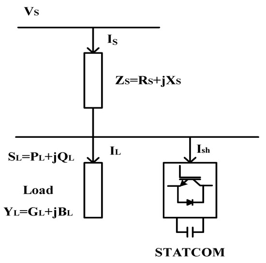
Figure 1.
Principle of STATCOM voltage stability improvement.
Figure 2 is a vector diagram of voltage drop caused by the line impedance . Depending on the power system situation, STATCOM operates in the form of supplying reactive power (Capacitive Reactive Power) or absorbing the reactive power (Inductive Reactive Power), or in the form of supplying the active power or absorbing the active power. When a voltage drop occurs at the receiving end because of the inductance of the line impedance , the reactive power compensation current is supplied for compensating the voltage drop of the system. A voltage drop is generated by resistance component and reactance component , and before compensation the load current angle is . and can be kept the same through current compensation, and the load current angle is compensated to . The reactive power compensation current can be expressed as Equation (4) [29]:
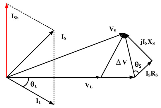
Figure 2.
Vector Diagram of STATCOM Power Quality Compensation.
When the loads is an inductive load, STATCOM can make a capacitive current and scale it to change the phase angle of . By adjusting according to the compensation current of STATCOM, the voltage of the load stage and the magnitude of the bus voltage can be kept constant.
3. Proposed Virtual STATCOM System
DGs, such as solar power and wind power ESS, are connected to the power system via inverters, and a number of inverters connected to the DG are capable of outputting active power and reactive power. However, distributed power sources currently connected to the grid operate as the power sources and supply only active power. The reactive power generated in the power system is not compensated for. Since each inverter is individually and independently controlled, it is difficult to effectively compensate for the reactive power of the power system. The proposed Virtual STATCOM system can effectively control the reactive power of the power system with an integrated control rather than the independent control of multiple inverters of distributed power sources connected to the power system. Since no new facilities are installed for compensating for the reactive power, the installation cost can be economically feasible. Furthermore, compensating for the reactive power of the PCC stage to 0 can be expected to improve voltage stability, to remove harmonics, to increase transmission capacity, and to enhance the lifespan of facilities. Figure 3 shows the configuration schematic of Virtual STATCOM.
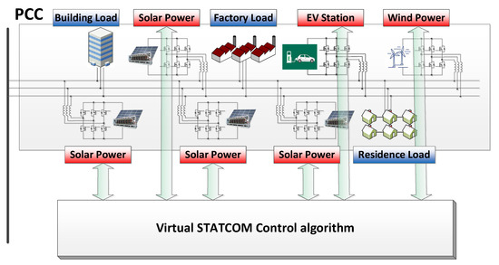
Figure 3.
Virtual STATCOM configuration schematic.
3.1. Configuration of Virtual STATCOM
In general, STATCOM is a facility that improves the stability of the power system by controlling the reactive power of the connection point. When multiple DG inverters connected to the system independently compensate for reactive power at the connection point, like in the case of a general STATCOM, the system stability may deteriorate because of the hunting that occurs during the control operation. The purpose of this paper is to compensate for or control the reactive power at a designated location in the system by controlling the inverters of DGs connected to multiple connection points. That is, it is expected that the proposed Virtual STATCOM can improve the stability of the entire power system by controlling reactive power at a desired point, such as a weak or important location of the connection or distribution end of the transmission and distribution system, like the PCC of the power system. In this paper, PCC was designated as the control reference point that is the connection point of transmission and distribution, and the Virtual STATCOM integrated control algorithm was configured by the linear programming. To improve the voltage stability of the PCC, the reactive power of the PCC should be controlled to 0. The reactive power of the PCC stage is divided into a component generated by the line impedance and a component generated by the load. To compensate for the reactive power of the PCC stage to 0, it is necessary to compensate for the reactive power while considering both causes of the reactive power.
Figure 4 shows the configuration of the Virtual STATCOM system. Three solar power plants are connected between the voltage source and load. It is assumed that each solar power plant has a different distance from the bus of the PCC stage, and the amounts of connected load, solar power plant capacities, and power generation amounts are different from each other. The inverter of the solar power plant can output the active power and the reactive power as much as the rated capacity S. When there is room in the inverter output rated capacity after supplying the active power P generated by the PV panel to the grid, the reactive power can be supplied. The inverter rated capacity S of a solar power plant can be expressed as Equation (5):
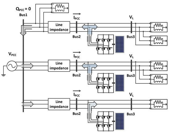
Figure 4.
Configuration Scheme of the Virtual STATCOM System.
The Virtual STATCOM integrated control algorithm selects the inverter closest to the PCC to give it priority, and when the amount of the reactive power that can be output is insufficient, the compensation will be performed from the inverter as the next priority.
Figure 5 shows the configuration of the integrated control algorithm of Virtual STATCOM. By combining Solar Station, PMU, and Distance Information, the Virtual STATCOM Control algorithm is configured based on LP, and the control reference of the inverter is derived. A plurality of inverters improves the voltage stability by the reactive power compensation of the PCC stage.
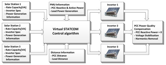
Figure 5.
Configuration of Virtual STATCOM Integrated Control Algorithm.
3.2. Scheme of Virtual STATCOM Control
To configure the integrated control algorithm of Virtual STATCOM based on LP, the decision variables, the objective functions, and the constraints must be selected according to the control purpose [30].
3.2.1. Decision Variable
The decision variable is for setting the variable that is the control criterion of the LP. Since the purpose of the Virtual STATCOM is to output the inverter reactive power compensation reference, the inverter reactive power output amount was selected as a decision variable.
Decision Variable = Qinv: Inverter Reactive Power Output
3.2.2. Objective Function
The objective function is for setting the goal of the decision variable. As the distance from the PCC terminal increases, the loss caused by the line impedance increases, so it is designated as the goal to use an inverter with a shorter distance. To select a minimum distance, a point where the product of the decision variable and the weight is minimized is set as the optimal point.
where, refers to the distance weight of inverter, and refers to the line distance of inverter from the PCC end point. is decided by the following equation as a consideration of the distance between the inverter and the PCC end point.
3.2.3. Constraints
The constraints determine the minimum compensation value and the maximum compensation value for the decision variable of the inverter to determine the reactive power that is to be compensated for by the inverter. The constrains for the minimum and maximum amounts of the inverter reactive power output can be expressed as Equation (7):
where = Minimum of Inverter Reactive Power Compensation (var), and = Maximum of Inverter Reactive Power Compensation (var).
When the output of the inverter is maximized, the life of the inverter rapidly decreases, so the maximum output of the inverter is limited to 80%. To determine the amount of the reactive power compensation of the inverter, the minimum and maximum amounts of reactive power compensation of the inverter should be set as the constraints. Constraints are determined in consideration of the effective load amount of the inverter terminal, the reactive load amount of the inverter terminal, the rated capacity, the inverter active power generation amount, and the inverter generation rated limit.
means the maximum reactive power compensation amount that can be compensated for by the inverter. The maximum amount of inverter reactive power compensation is determined by considering the rated capacity of the inverter, the amount of active power currently being generated by the inverter, and the inverter power generation rating limit.
where means the minimum reactive power compensation amount that can be compensated by the inverter. The reactive power can be expressed in negative or positive number according to inductivity and capacity, so the negative number of the maximum amount of compensable reactive power is determined as the minimum compensable amount of the inverter.
Considering the reactive power generated in the PCC stage, the reference value of the reactive power compensation for each inverter is calculated. The reactive power of PCC stage consists of the reactive power generated by line impedance and the reactive power generated by load. When the total amount of reactive power generated in the PCC stage is equal to the total amount of reactive power compensated for by the inverter, the reactive power in the PCC stage is compensated to 0.
Table 1 shows the parameters for configuring the Virtual STATCOM system.

Table 1.
Virtual STATCOM System Parameters.
Figure 6 shows the Virtual STATCOM Integrated Control Algorithm Diagram. The compensation algorithm is configured through five steps. Step 1 measures the parameter values required for Virtual STATCOM configuration. Step 2 determines the reactive power compensation’s possible range based on the measured parameter value. Step 3 determines the optimal reference for reactive power compensation using LP. Step 4 performs reactive power compensation through an inverter and measures the reactive power of PCC. If the reactive power of PCC converges to 0, proceed to Step 5. If it does not converge, return to Step 1 and perform the algorithm again. Step 5 is the step of storing the reactive power compensation value determined by Steps 1–4. Equation (13) shows the reactive power compensation value of the algorithm diagram, where is the stored PCC reactive power value of Step 5.
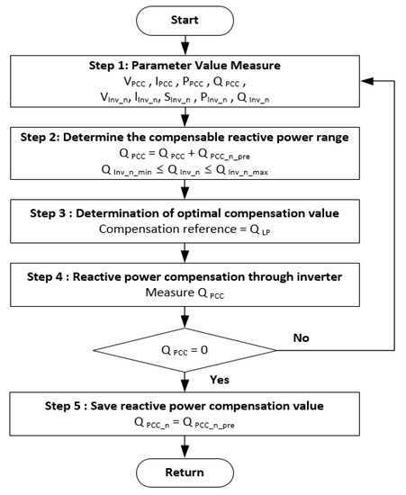
Figure 6.
Virtual STATCOM Integrated Control Algorithm Diagram.
If the reactive power compensation value is not saved and the algorithm is executed, only the value of is compensated for when a load change occurs, and PCC reactive power is generated to as much as the value.
4. Virtual STATCOM Simulation
To verify the Virtual STATCOM’s performance, simulation was conducted using Matlab Simulink and the Real Time Simulator (OPAL-RT) OP5700.
The Real Time Simulator is a simulation technology that proceeds by setting the simulation time to be same as the real time. By running the simulation under the same conditions as in reality, problems that do not appear in the off-line simulation can be derived, and the reliability of the simulation can be improved. By establishing a virtual controller and a virtual plant in the target PC, a Model In the Loop Simulation (MILS) was performed. The plant of the simulation model was designated as Master, and the controller was designated as Slave, and tow cores were used. The result data of the simulation were output via the target PC. Figure 7 shows the Simulation Model of Virtual STATCOM.
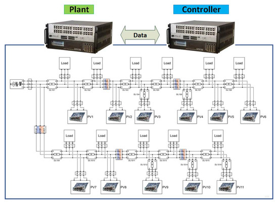
Figure 7.
Virtual STATCOM Simulation Model.
The system model used in the simulation was that of Anseong, in South Korea. The distributed resources connected to the Anseong area, and the system diagram of the entire systems was made equivalent by integrating the system load into sections as shown in Figure 8. Table 2 shows the DG inverter and load data of the Anseong area system.
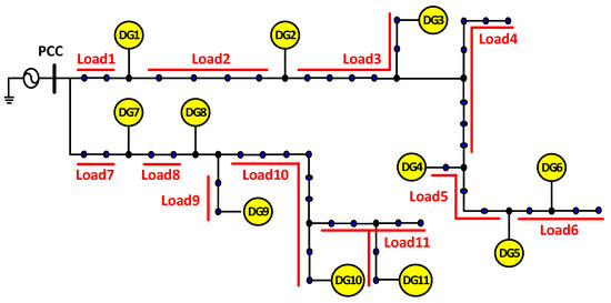
Figure 8.
Virtual STATCOM Simulation Grid Diagram.
Table 2.
Virtual STATCOM Simulation Model Parameters.
For the simulation system model, the simulation was performed with equivalence to a system including one voltage power source, 11 DGs, and 11 loads. The power source output AC of 22.9kV, 60Hz via the Three Phase Source. The load was simulated by dividing the section of the system using the three-phase parallel RLC load and making the load within the section equivalent to one load. The load between PCC and DG1 was set as , and the subsequent loads were designated as by grouping the loads between DGs. All loads used in the simulation were divided into 11 sections. To perform compensation considering the distance between the PCC terminal and the DGs, the line impedance according to the distance was made equivalent using the PI Section Line.
For the simulation sample time, the simulation was conducted by dividing it into three categories: the power system, the inverter controller, and the algorithm according to the purpose. The sample time of the power system was set to 50 (s) for simulating the instantaneous system change situation, and the sample time for the inverter controller was set to 100 (s). The Virtual STATCOM integrated control algorithm sample time was set to 0.1 (s) in consideration of the data measurement period of the PMU.
Table 3 shows the Virtual STATCOM simulation scenario. This table indicates whether the Virtual STATCOM Control Algorithm operates according to the simulation time, and also indicates the load change time. The data for the load change are shown in Table 4. For the simulation time of 0~1 (s), a situation, in which the Virtual STATCOM Control Algorithm does not operate and the load fluctuation does not occur, is simulated.
Table 3.
Virtual STATCOM Simulation Scenario.
Table 4.
Virtual STATCOM Simulation Model Parameters (Load Variation).
For the simulation time of 1 (s), the load variation situation was simulated. generated a variation of +0.7 (Mvar) in 1 (s), generated +0.3 (Mvar), generated −0.25 (Mvar), generated +1.1 (Mvar), generated +2.1 (Mvar), generated +0.2 (Mvar), and generated the variation of −0.15 (Mvar), so the reactive power of PCC generated the variation of +4 (Mvar). At the simulation time of 2 (s), had the variation of −0.4 (Mvar), had −0.2 (Mvar), had +0.5 (Mvar), had −0.3 (Mvar), had −0.5 (Mvar), had +1 (Mvar), had +0.2 (Mvar), had −2 (Mvar), and had the variation of −0.3 (Mvar), so the reactive power of PCC having the variation of −2 (Mvar) was simulated.
Figure 9 shows the simulation results, assuming that power quality compensation using the Virtual STATCOM control algorithm is not conducted. During the simulation run time of 0~1 (s), the distributed power supply was connected to the system and the steady state operation was in progress. The voltage of PCC has a voltage drop of 22.87 kV caused by the inductance L and resistance R. In PCC reactive power, the ground reactive power of 5.8 (Mvar) is generated by line impedance components and non-linear loads. In 1~2 (s), it is found that the reactive power of +4 (Mvar) is increased by the load variation, and the voltage of PCC is 22.85 kV, so that the voltage drop is increased. In 2~3 (s), the occurrence of voltage transients and reactive power of −2 (Mvar) were reduced because of the increase of the capacitive load, and reactive power of 7.8 (Mvar) is generated at the PCC point, and a voltage drop of 22.86 kV occurs.
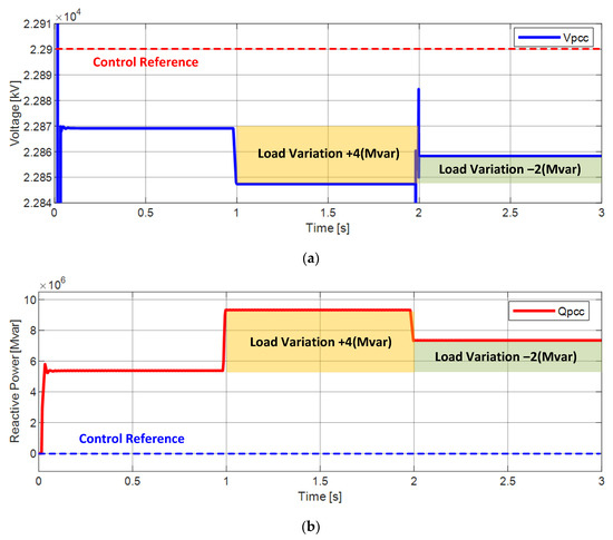
Figure 9.
PCC Variation according to the Load Variation of Virtual STATCOM (Before Compensation by Algorithm) (a) PCC Voltage, (b) PCC Reactive Power.
Figure 10 shows the power quality compensation simulation results using the Virtual STATCOM control algorithm. Virtual STATCOM was configured using inverters of multiple DGs connected to the system, and the optimum compensation command value of inverters was controlled using LP. Each inverter was controlled for the purpose of improving voltage stability by compensating for the reactive power of PCC to 0. Figure 10a,b show the PCC voltage and reactive power, and Figure 10c shows the amount of reactive power compensation of Virtual STATCOM inverters.
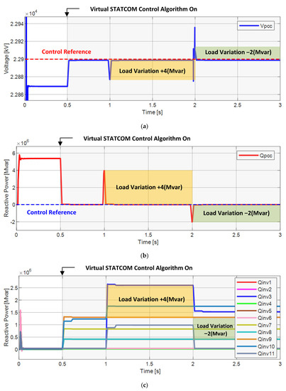
Figure 10.
Virtual STATCOM Power Quality Compensation (a) PCC Voltage, (b) PCC Reactive Power, (c) Compensation Amount for Inverter Reactive Power.
As the simulation time of 0~0.5 (s) is the status in which the Virtual STATCOM algorithm is not applied, the power quality is not compensated for, so the reactive power of the PCC stage is about 5.8 (Mvar). Furthermore, the voltage at the PCC terminal is 2.287 kV due to the line and load impedance components, and a voltage drop has occurs. It was found that when the Virtual STATCOM control algorithm operated at 0.5 (s), the reactive power of PCC stage converged to 0 by the reactive power compensation, and the voltage of the PCC stage was compensated to 22.9 kV. At 1 (s), as the reactive power of PCC increased with +4 (Mvar) by Load Variation, a voltage drop of 22.88 kV occurred, but the reactive power and the voltage of the PCC were compensated for to the reference values by the Virtual STATCOM integrated algorithm. For 1~2 (s), there was no change. At 2 (s), Load Variation occurred, and the capacitance reactive power of −2 (Mvar) occurred in PCC, so the voltage rose to 22.93 kV. However, it was found that the reactive power of the PCC stage was compensated to 0 and the voltage was sustained to 22.9 kV by the integrated control algorithm.
Figure 11 shows the amount of reactive power compensation of Virtual STATCOM inverters 1–11. To control the reactive power of the PCC to 0 using the inverter integrated control, the reactive power compensation amount of the inverters was determined in consideration of the available reactive power amount of the inverter and the distance between the PCC and the inverter. Since inverters have different distances from the PCC, the loss caused by the line impedance may increase when the long-distance inverter compensates for a large amount. Therefore, compensation was carried out by selecting an inverter that is relatively close to the PCC as the compensation priority. In addition, the rated capacity is different for each connected inverter, and the amount of the reactive power that can be output is different because the amount of power currently being output is different. Therefore, by considering the rating and remaining capacity of each inverter, the optimum compensation command is generated with priority according to the maximum amount of reactive power and distance.
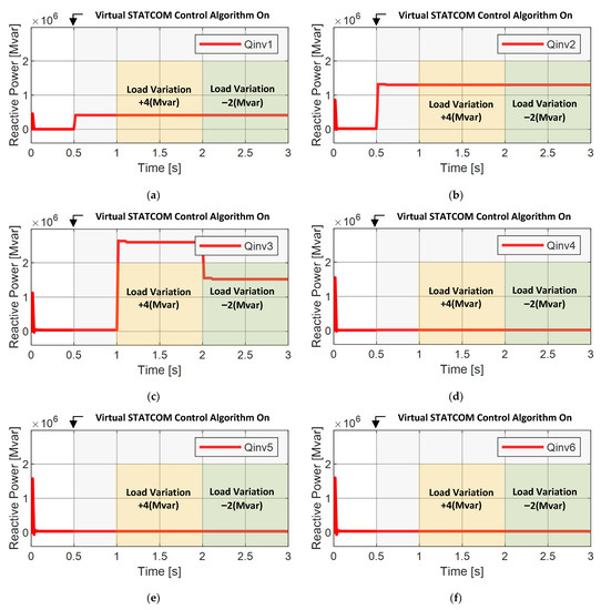
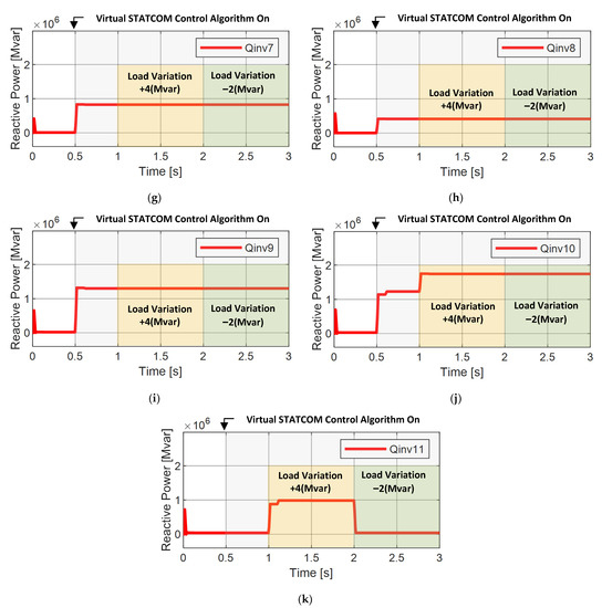
Figure 11.
11 Reactive Power Compensation Amount of Virtual STATCOM Inverter 1: (a) Inverter 1, (b) Inverter 2, (c) Inverter 3, (d) Inverter 4, (e) Inverter 5, (f) Inverter 6, (g) Inverter 7, (h) Inverter 8, (i) Inverter 9, (j) Inverter 10, (k) Inverter 11.
In the time of 0~0.5 (s), the Virtual STATCOM control algorithm does not operate, so the Virtual STATCOM inverters are not outputting the reactive power. The control algorithm operates at 0.5 (s), and the reactive power compensation is carried out in consideration of the distance of the inverter to the maximum reactive power output. The reactive power compensation is carried out by dividing reactive power 5.8 (Mvar) generated in PCC by inverters 1, 2, 7, 8, 9, and 10. Inverter 1 compensated 0.4 (Mvar) reactive power, Inverter 2 compensated 1.35 (Mvar), Inverter 7 compensated 0.9 (Mvar), Inverter 8 compensated 0.45 (Mvar), Inverter 9 compensated 1.4 (Mvar), and Inverter 10 compensated 1.2 (Mvar). In Load Variation 1 (s), inverters 1, 2, 3, 7, 8, 9, 10 and 11 divided PCC reactive power of 9.8 (Mvar), so Inverter 1 compensated 0.4 (Mvar), Inverter 2 compensated 1.35 (Mvar), Inverter 3 compensated 2.5 (Mvar), Inverter 7 compensated 0.9 (Mvar), Inverter 8 compensated 0.45 (Mvar), Inverter 9 compensated 1.4 (Mvar), Inverter 10 compensated 1.8 (Mvar), and Inverter 11 compensated 1 (Mvar). In the case of a load variation of 2 (s), inverters 1, 2, 3, 7, 8, 9 and 10 divided PCC reactive power of 7.8 (Mvar), so Inverter 1 compensated 0.4 (Mvar), Inverter 2 compensated 1.35 (Mvar), Inverter 3 compensated 1.5 (Mvar), Inverter 7 compensated 0.9 (Mvar), Inverter 8 compensated 0.45 (Mvar), Inverter 9 compensated 1.4 (Mvar), and Inverter 10 compensated 1.8 (Mvar).
5. Conclusions
This paper proposed a Virtual STATCOM Configuration and Control method that operates like a single STATCOM based on multiple DGs connected to the system. The conventional STATCOM has the following demerits: as it is installed in the power transmission/transformation system, it is hard to operate while considering the power quality of the distribution system; when installing STATCOM in the distribution system, it is hard to select the installation location because of the complexity of the distribution system; and when proper positioning is not considered, the economic feasibility of STATCOM will be reduced. The Virtual STATCOM solves the problem of installation location selection with the configuration that includes a DG inverter connecting to the grid system, and enhances the economic feasibility by using the equipment connected to the existing system.
Virtual STATCOM is controlled using the operating principle of the existing STATCOM. It improves voltage stability through reactive power compensation. Multiple DGs connected to the grid were integrated and controlled through an LP-based algorithm. As a result of the simulation, we confirmed that the voltage drop occurred because of the line impedance and load impedance components before compensation through the Virtual STATCOM integrated control algorithm. As a result of the compensation using the Virtual STATCOM algorithm, we confirmed that the voltage stability was improved through the reactive power compensation of the PCC. To verify the performance, a simulation was conducted based on a real-time simulator. The off-line simulation results and the real-time simulation results are the same, so we verified that there is no problem in an environment similar to the real one.
Author Contributions
Conceptualization, T.-S.P. and S.-H.P.; methodology, B.-H.A. and J.-D.P.; software, S.-H.P. and T.-H.K.; validation, J.-H.P. and M.-J.L.; formal analysis, S.-H.P.; writing—original draft preparation, S.-H.P.; review and editing, T.-S.P. and S.-H.P. All authors have read and agreed to the published version of the manuscript.
Funding
This work was supported by the Gwangju Jeonnam Local Energy Cluster Manpower Training of the Korea Institute of Energy Technology Evaluation and Planning (KETEP) grant funded by the Korean government’s Ministry of Knowledge Economy (20214000000560).
Conflicts of Interest
The authors declare no conflict of interest.
References
- Khalilpour, K.R.; Vassallo, A. Community Energy Networks with Storage: Modeling Frameworks for Distributed Generation; Springer: Berlin/Heidelberg, Germany, 2016. [Google Scholar]
- Amini, M.H.; Nabi, B.; Haghifam, M.-R. Load management using multi-agent systems in smart distribution network. In Proceedings of the 2013 IEEE Power & Energy Society General Meeting, Vancouver, BC, Canada, 21–25 July 2013; pp. 1–5. [Google Scholar]
- Hung, D.Q.; Mithulananthan, N.; Bansal, R. Analytical strategies for renewable distributed generation integration considering energy loss minimization. Appl. Energy 2013, 105, 75–85. [Google Scholar] [CrossRef]
- Rueda-Medina, A.C.; Padilha-Feltrin, A. Distributed generators as providers of reactive power support—A market approach. IEEE Trans. Power Syst. 2012, 28, 490–502. [Google Scholar] [CrossRef]
- Adefarati, T.; Bansal, R. Reliability assessment of distribution system with the integration of renewable distributed generation. Appl. Energy 2017, 185, 158–171. [Google Scholar] [CrossRef]
- Mithulananthan, N.; Hung, D.Q.; Lee, K.Y. Intelligent Network Integration of Distributed Renewable Generation; Springer: Berlin/Heidelberg, Germany, 2017. [Google Scholar]
- Hingorani, N.G.; Gyugyi, L.; El-Hawary, M. Understanding FACTS: Concepts and Technology of Flexible AC Transmission Systems; IEEE Press: New York, NY, USA, 2000; Volume 1. [Google Scholar]
- Hingorani, N.G. FACTS-flexible AC transmission system. In Proceedings of the International Conference on AC and DC Power Transmission, London, UK, 17–20 September 1991; IET: London, UK, 1991; pp. 1–7. [Google Scholar]
- Hingorani, N.G. Flexible AC transmission. IEEE Spectr. 1993, 30, 40–45. [Google Scholar] [CrossRef]
- Hingorani, N.G. High power electronics and flexible AC transmission system. In Proceedings of the American Power Conference, Chicago, IL, USA, 18–20 April 1988. [Google Scholar]
- Rao, P.; Crow, M.; Yang, Z. STATCOM control for power system voltage control applications. IEEE Trans. Power Deliv. 2000, 15, 1311–1317. [Google Scholar] [CrossRef] [Green Version]
- Tuzikova, V.; Tlusty, J.; Muller, Z. A novel power losses reduction method based on a particle swarm optimization algorithm using STATCOM. Energies 2018, 11, 2851. [Google Scholar] [CrossRef] [Green Version]
- Bhat, M.V.; Manjappa, N. Flower pollination algorithm based sizing and placement of DG and D-STATCOM simultaneously in radial distribution systems. In Proceedings of the 2018 20th National Power Systems Conference (NPSC), Tiruchirappalli, India, 14–16 December 2018; pp. 1–5. [Google Scholar]
- Casey, L.F.; Schauder, C.; Cleary, J.; Ropp, M. Advanced inverters facilitate high penetration of renewable generation on medium voltage feeders-impact and benefits for the utility. In Proceedings of the 2010 IEEE Conference on Innovative Technologies for an Efficient and Reliable Electricity Supply, Waltham, MA, USA, 27–29 September 2010; pp. 86–93. [Google Scholar]
- Turitsyn, K.; Sulc, P.; Backhaus, S.; Chertkov, M. Options for control of reactive power by distributed photovoltaic generators. Proc. IEEE 2011, 99, 1063–1073. [Google Scholar] [CrossRef] [Green Version]
- Smith, J.; Sunderman, W.; Dugan, R.; Seal, B. Smart inverter volt/var control functions for high penetration of PV on distribution systems. In Proceedings of the 2011 IEEE/PES Power Systems Conference and Exposition, Phoenix, AZ, USA, 20–23 March 2011; pp. 1–6. [Google Scholar]
- Schauder, C. Advanced Inverter Technology for High Penetration Levels of PV Generation in Distribution Systems; National Renewable Energy Lab (NREL): Golden, CO, USA, 2014. [Google Scholar]
- Siavashi, E.M. Smart PV Inverter Control for Distribution Systems. Ph.D. Thesis, The University of Western Ontario, London, ON, Canada, 2015. [Google Scholar]
- Varma, R.K.; Rahman, S.A.; Mahendra, A.; Seethapathy, R.; Vanderheide, T. In Novel nighttime application of PV solar farms as STATCOM (PV-STATCOM). In Proceedings of the 2012 IEEE Power and Energy Society General Meeting, San Diego, CA, USA, 22–26 July 2012; pp. 1–8. [Google Scholar]
- Varma, R.K.; Rahman, S.A.; Vanderheide, T. New control of PV solar farm as STATCOM (PV-STATCOM) for increasing grid power transmission limits during night and day. IEEE Trans. Power Deliv. 2014, 30, 755–763. [Google Scholar] [CrossRef]
- Varma, R.K.; Maleki, H. PV Solar System Control as STATCOM (PV-STATCOM) for Power Oscillation Damping. IEEE Trans. Sustain. Energy 2019, 10, 1793–1803. [Google Scholar] [CrossRef]
- Varma, R.K.; Khadkikar, V.; Seethapathy, R. Nighttime application of PV solar farm as STATCOM to regulate grid voltage. IEEE Trans. Energy Convers. 2009, 24, 983–985. [Google Scholar] [CrossRef]
- Wandhare, R.G.; Agarwal, V. Novel stability enhancing control strategy for centralized PV-grid systems for smart grid applications. IEEE Trans. Smart Grid 2014, 5, 1389–1396. [Google Scholar] [CrossRef]
- Shah, R.; Mithulananthan, N.; Lee, K.Y. Large-scale PV plant with a robust controller considering power oscillation damping. IEEE Trans. Energy Convers. 2012, 28, 106–116. [Google Scholar] [CrossRef]
- Luo, L.; Gu, W.; Zhang, X.-P.; Cao, G.; Wang, W.; Zhu, G.; You, D.; Wu, Z. Optimal siting and sizing of distributed generation in distribution systems with PV solar farm utilized as STATCOM (PV-STATCOM). Appl. Energy 2018, 210, 1092–1100. [Google Scholar] [CrossRef]
- Kundur, P. Power system stability. In Power System Stability and Control; CRC press: Boca Raton, FL, USA, 2007; p. 10. [Google Scholar]
- Hossain, J.; Mahmud, A. Large Scale Renewable Power Generation; Springer: Singapore, 2014. [Google Scholar]
- Tabatabaei, N.M.; Aghbolaghi, A.J.; Bizon, N.; Blaabjerg, F. Reactive Power Control in AC Power Systems; Springer: Cham, Switzerland, 2017. [Google Scholar]
- Arulampalam, A.; Ekanayake, J.B.; Jenkins, N. Application study of a STATCOM with energy storage. IEE Proc.-Gener. Transm. Distrib. 2003, 150, 373–384. [Google Scholar] [CrossRef]
- Luenberger, D.G.; Ye, Y. Linear and Nonlinear Programming; Springer: New York, NY, USA, 2008; Volume 116. [Google Scholar]
Publisher’s Note: MDPI stays neutral with regard to jurisdictional claims in published maps and institutional affiliations. |
© 2022 by the authors. Licensee MDPI, Basel, Switzerland. This article is an open access article distributed under the terms and conditions of the Creative Commons Attribution (CC BY) license (https://creativecommons.org/licenses/by/4.0/).