Non-Intrusive Load Monitoring of Household Devices Using a Hybrid Deep Learning Model through Convex Hull-Based Data Selection

Abstract

The availability of smart meters and IoT technology has opened new opportunities, ranging from monitoring electrical energy to extracting various types of information related to household occupancy, and with the frequency of usage of different appliances. Non-intrusive load monitoring (NILM) allows users to disaggregate the usage of each device in the house using the total aggregated power signals collected from a smart meter that is typically installed in the household. It enables the monitoring of domestic appliance use without the need to install individual sensors for each device, thus minimizing electrical system complexities and associated costs. This paper proposes an NILM framework based on low frequency power data using a convex hull data selection approach and hybrid deep learning architecture. It employs a sliding window of aggregated active and reactive powers sampled at 1 Hz. A randomized approximation convex hull data selection approach performs the selection of the most informative vertices of the real convex hull. The hybrid deep learning architecture is composed of two models: a classification model based on a convolutional neural network trained with a regression model based on a bidirectional long-term memory neural network. The results obtained on the test dataset demonstrate the effectiveness of the proposed approach, achieving F1 values ranging from 0.95 to 0.99 for the four devices considered and estimation accuracy values between 0.88 and 0.98. These results compare favorably with the performance of existing approaches.

1. Introduction

The world’s ever-increasing energy consumption and ongoing dependency on fossil fuel-based energies have created significant environmental concerns, particularly in terms of carbon dioxide (CO₂) emissions [1]. Focusing on the European country hosting the current case-study household, Portugal, greenhouse gas (GHG) emissions increased by 13% from 2014 to 2018 as a result of increased economic activity and a high proportion of fossil fuels in its energy supply [2]. In 2019, imported fossil fuels represented 76% of Portugal’s primary energy (6% coal, 24% natural gas, and 43% oil) [2]. Low-carbon economies have emerged as the focus of worldwide attention in order to minimize energy consumption and greenhouse gas emissions [3]. The targets set by the EU for 2030 include a minimum 32% share of renewable energy consumption in the energy mix, a minimum of 32.5% energy savings, and a 40% reduction in greenhouse gas emissions compared to 1990 levels [4]. Portugal was among the first countries in the world to set carbon neutrality goals for the year 2050 [2]. The focus is on minimizing dependency on imported fossil fuels and effective energy demand management.

At a global perspective, the building sector accounts for the largest worldwide electricity consumption, for roughly 32% of overall energy consumption, and for 19% of total energy-related greenhouse gas emissions [5,6]. Residential energy consumption accounted for 25.71% of the EU’s total final energy consumption, making it the second most energy-intensive sector after transport [7]. There is an urgent need to counteract the upward trend in building energy use. The European Union (EU) is making considerable efforts to prevent global warming by enacting several key policies [8]. Therefore, to meet global and EU carbon reduction targets, research efforts are required at the building sector to lower its high contribution to global energy consumption. [9].

Since 2010, the amount of electricity consumed by household devices has risen by about 3% per year. In 2019, household device electricity consumption exceeded 3000 TWh, accounting for 15% of worldwide final electricity demand [10]. Energy awareness can help to reduce energy consumption in the households [11]. Hence, occupant behaviors have a significant role in increasing energy efficiency. Moreover, if end-users can be notified in real-time and explicitly about the consumption of each appliance in their home, unnecessary energy usage can be reduced [12,13,14].

The availability of smart meters and IoT technology has opened new opportunities, ranging from monitoring electrical energy to extracting various types of information related to household occupancy, as well as the frequency of usage of different appliances. Device monitoring can be performed by installing one or a set of sensors in each device of interest [15], which is known as intrusive load monitoring (ILM). It allows for accurate detection of the operating state of each appliance [16]. However, its deployment requires complex installation and configuration of multiple sensors, especially when multiple appliances are involved in the monitoring scenario [14]. It also entails a high cost, and its intrusive nature leads to some privacy concerns [11]. All these disadvantages limit its practical use.

On the other hand, non-intrusive load monitoring (NILM) is one of the most promising options for energy disaggregation. It allows users to separate the usage of each device in the house by using the total aggregated power signals collected from a smart meter that is typically installed in a household, while protecting user privacy [11,17]. The goal of NILM is to estimate the specific consumption of each appliance in the house based on aggregated data collected by a smart meter. Moreover, it enables monitoring domestic appliance usage without the need to install individual sensors for each device, thus minimizing electrical system complexities and associated costs [18]. According to [19], basic appliances, such as a washing machine, refrigerator, and oven, account for more than 30% of household consumption. The identification of these types of devices in the aggregate data is, however, challenging due to their complex feature patterns.

Four types of devices are categorized in the literature [14,20]. The first category (type I) comprises two state (ON-OFF) appliances such as toasters and light bulbs. The finite state machines (FSM) or multi-state appliances categorized as type II devices include appliances such as washing machines and fridges. Type III includes continuously variable consumer devices such as power tools and dimmers. Finally, permanent consumer appliances such as smoke alarms are categorized as type IV. The challenge for NILM algorithms is the identification of all types of devices with good performances. Type I devices are easier to disaggregate due to their basic architecture. The disaggregation of the other types of devices (Type II to Type IV) is still a challenging issue for NILM methods [11].

The NILM process was described for the first time in [21]. Hart proposed that, based on the entire aggregate energy usage monitored using a sensor installed on the main power panel, changes of the devices could be detected by applying an appropriate statistical test to the collected data. Subsequently, the transitions were identified using a convenient features vector, and finally, the identification of each device was performed using supervised or unsupervised approaches [14], with supervised techniques being typically more efficient than unsupervised approaches [11,22].

The initial phase in every NILM algorithm is data gathering. Indeed, the frequency with which the smart meter collects data determines the challenges and applications that the NILM algorithm will encounter [23]. Data may be acquired at either a high frequency sampling rate, in the range of kHz, or using a low frequency (1 Hz or less) sampling rate. Features such as harmonics, transients, and V-I trajectory are used to detect the appliance contribution in high frequency approaches [24,25,26]. On the other hand, methods based on low frequency sampling rates generally employ power features such as active power (P), reactive power (Q), or apparent power (S) [27,28,29,30]. High frequency approaches have the disadvantage of making data transmission and storage difficult, as well as being costly in terms of hardware and software complexity. Low frequency techniques, on the contrary, are the effective choice in NILM applications since they allow the use of commercial smart meter resources without the need for additional equipment [31].

The interest in NILM research has been diversified since its earliest days. The total power series was first examined to find power changes that reflect device switching events, and then these occurrences attributed to specific devices [21,32,33]. A later interest in NILM research has given rise to different variants of hidden Markov models [34,35,36,37,38]. More recently, the huge success of deep learning in the fields of vision and natural language processing has led to a great interest in these approaches for NILM, which started with the works [13,39]. A comprehensive review of NILM methods, including existing problems, can be found in [11]. A discussion about current NILM methods will be detailed in Section 2.

Despite the numerous NILM research reported in literature, many problems persist. These challenges include, for instance, poor detection performance, particularly for low power and multistate devices, lesser scalability to detect newly added devices, and the need to generate more datasets [14]. In order to tackle these challenges, deep learning algorithms may be a suitable tool for improving the accuracy and efficiency of energy disaggregation techniques [13]. This paper proposes an NILM framework based on low frequency power data. The framework employs a convex hull data selection method and a hybrid deep learning architecture. The main contributions of this research may be summarized as follows:

• An NILM framework based on private house data gathering in a real-life situation, using low frequency sampling rate of 1 Hz.
• A randomized approximation convex hull data selection approach using sliding windows of active and reactive power. It is based on the selection of the most informative vertices of the real convex hull and has the advantage of reducing memory needs of the learning algorithms.
• A hybrid deep learning architecture composed of two models. A classification model based on a convolutional neural network trained with a regression model based on a bidirectional long-term memory neural network.
• The results obtained with the proposed NILM framework on the test dataset demonstrate the effectiveness of the proposed approach, as well as achieving better results than existing approaches.

The rest of the paper is organized as follows: Section 2 provides a brief overview of existing NILM algorithms. Section 3 describes the problem formulation, the convex hull data selection approach used, the hybrid deep learning models, the case study employed, and the evaluation metrics employed. Results and discussion are presented in Section 4. Section 5 concludes the paper.

2. Related Works

Going back to the genesis of the NILM concept [21], the authors demonstrated that the appliances exhibit distinct power consumption signatures. In their approach, on/off events were utilized to identify the operating state of specific devices in the aggregate active and reactive powers. Nonetheless, the method had difficulty identifying some types of devices (type II, type III, and type IV). Following that, numerous alternative approaches were investigated in order to tackle the NILM problem. Hidden Markov Models and its variants have been widely explored early on. Indeed, an additive Factorial Hidden Markov Model for non-intrusive load monitoring was proposed in [37]. The authors used an approach for exploiting the additive structure of the Factorial Hidden Markov Model (FHMM) to construct an estimate inference approach that utilizes an efficient convex quadratic programming relaxation. The proposed approach performed well while maintaining a reasonable computing complexity. The authors of [40] examined several Hidden Markov Models (HMM). In their study, Conditional FHMM (CFHMM), Hidden Semi-Markovian Factorial Model (HSMM), and the FHSMM/CFHMM combination using multi-dimensional characteristics were explored. These researchers used actual steady state power signal in the low frequency data and demonstrated that unsupervised methods could be utilized to identify devices non-invasively. The authors of [36] proposed a factorial hidden Markov Model for NILM. They concentrated on detecting the binary and multistate operation of devices using appropriate feature sets. They showed how feature concatenation can improve the accuracy of device identification. In [41], prior models of generic device types are adjusted to device instances based only on fingerprints collected from the aggregate load. The adjusted device models are then used to predict the load of each device, which is then removed from the total load. This procedure is repeated until all devices with known prior behavior models have been disaggregated. They showed that the proposed approach performs as well as when using sub-metered training data. The authors of [34] presented a sparse Viterbi approach that uses a super-state HMM to preserve load correlations and detect multi-state loads while offering computationally efficient inference. They evaluated their model using a low frequency sampling rate and showed that their model could run in real-time on a low-cost embedded CPU. The authors of [35] developed an Additive Factorial Approximate Maximum a Posteriori (AFAMAP) method. In their approach, active and reactive powers are used at a low frequency sampling rate. It entails modeling the value of each aggregated power sample as a combination of device operating states and then recreating the time series of state evolution for each finite state machine device. They demonstrated that the use of reactive power increases the performance of the technique. In [42], a machine learning approach for on-line non-intrusive load monitoring that combines unsupervised event-based profiling and Markov chain device load modeling is presented. In their approach, the event-based component detects events using contiguous and transient segments and matching and event clustering. The specific device model is created from a generic device model using the features obtained. The device model parameters are then used to create an additive FHMM for online disaggregation. They demonstrated that the suggested technique enables on-line detection while providing comparable prediction performance to non-online methods.

The complexity of HMM models and its variants grow exponentially as the number of target appliances grows. Moreover, their generalization and scalability abilities are problematic. Existing inference methods for state prediction are also extremely sensitive to local optima, hence, limiting their application in the real world [15]. Consequently, deep learning and machine learning techniques are suitable alternatives to address the NILM challenges. These include support vector machine [43,44,45], Decision Tree [46,47], K-nearest neighbors [48], K-means clustering [49], and graph signal processing [50,51] as worthwhile mentioning approaches.

The authors of [13] introduced deep learning approach for NILM. In their paper, three deep learning models were explored. These include denoising autoencoder, long short-term memory combined with a convolutional neural network, and a regression model that estimates the start time, end time, and the average power demand of each device. They modeled NILM as a denoising task, in which the target device power load represents the clean signal, and the aggregate load is the background ‘noise’ generated by the presence of other devices. They showed that the denoising autoencoder outperforms the FHMM and combinatorial optimization state of the art techniques. The authors of [52] presented a sequence to point approach. They employed a convolutional neural network, with the input being a window of aggregate active power and the output being a single point of the target appliance. They showed using the Reference Energy Disaggregation Data Set (REDD) [53] and UK Domestic Appliance-Level Electricity (DALE) [54] datasets that the sequence-to-point technique outperforms the sequence-to-sequence state of the art approaches. In [55], a deep learning based on the convolutional neural network, long-term short-term memory network, and random forest (RF) algorithm was presented. They investigated the concept of label correlations and tested their model on the Pecan Street [56] and REDD [49] datasets. A deep learning based on bidirectional long short-term memory model with a convolutional layer is proposed in [57]. The authors used a variety of electrical features to generate a multi-feature input. The model was validated using low frequency data from the publicly available datasets Electricity Consumption & Occupancy (ECO) [58] and UKDALE [54]. In the same paper, they proposed a post-processing algorithm to eliminate superfluous predicted sequences. They proved that using the post-processing technique, the model performs well. In [59], an NILM approach based on the deep convolutional neural network model using data augmentation to produce synthetic data is proposed. In their approach, the data augmentation method integrates on and off-durations of a target appliance from three datasets (ECO, REDD, and UKDALE) using a low frequency sampling rate. A unified and consistent synthetic aggregate and sub-meter profiles are then created. They showed that training the model on the produced synthetic data enhances its generalizability. The authors of [60] proposed a deep convolutional neural network based on data augmentation for type II devices. A post-processing algorithm was suggested to classify the activations estimated by the regression model. They demonstrated that using the suggested post-processing technique greatly enhances the model’s performance. The authors of [61] focused on improving NILM performance via a tailored attention mechanism. The approach is based on deep neural network architecture using the encoder-decoder framework. The proposed architecture consists of a regression subnetwork model combined with a classification subnetwork model. They suggested the use of convolutional and recurrent layers in the regression subnetwork to increase feature extraction and create better device models. They showed that the proposed approach improves model performances and generalization ability. Decision Tree and long short-term memory models are proposed in [46] to perform an event detection approach using transient signal. The latter was extracted in low frequency using active power signal. They showed that including the transient signal into the input signals improves the model’s performance. The authors of [18] proposed a multi-label classification approach based on a fully convolutional neural network. In their approach, the appliance states are classified using a features space enhanced by a temporal pooling module. The appliance power is estimated using the constant average value when the appliance is active. They showed that the proposed technique achieved good performance in recognizing the activation status of devices and estimating their power consumptions.

3. Materials and Methods

The main objective of energy disaggregation is to break down the house’s global aggregated data into specific contributions of each appliance. The purpose is to recognize each appliance operating state and to estimate its energy consumption contribution within the house’s total consumption. The problem can be stated as follows: given a sequence of aggregated data $X_t$= $\left\{x_1,\cdots ,x_T\right\}$, the task of NILM is to determine the contribution of each appliance I, $y_t^{\left(i\right)}=\left\{y_1^{\left(i\right)},\cdots ,y_T^{\left(i\right)}\right\},$ where I = {1, …, N} is the index of the appliance (from a set of N appliances), and t = {1, $\cdots$, T} is the time-index of the sequence with length T. The aggregated data can be expressed as the sum of the contribution of individual appliances plus an unknown part due to noise, represented by:

$$X_t={{\displaystyle \sum }}_1^N{y}_t^{\left(i\right)}+{\partial }_t$$

(1)

where ${\partial }_t$ is the noise term.

The contribution of an individual appliance $y_t^{\left(i\right)}$ is given by:

$$y_t^{\left(i\right)}=\psi (X_t)$$

(2)

where $\psi$ is the operator that, when applied to the whole aggregated data, gives the best estimate of the contribution of each individual appliance.

The task of obtaining an approximation of the operator $\psi$ may be addressed as a supervised learning problem [18]. This is the approach followed here, where the architecture of the proposed algorithm includes a convex hull-based data selection algorithm called ApproxHull, proposed in [62], and a hybrid deep neural network model.

The architecture of the hybrid network is made up of two subnetworks inspired in the work proposed in [61,63]. The approach makes use of an independent classification subnetwork that is trained jointly with the typical regression subnetwork. The network output is given by the combination of outputs of the two subnetworks. These learning approaches allow models to generalize efficiently for the original task by spreading parameters across related tasks [63]. Besides, deep neural networks tend to detect irrelevant activations that are not related to the target device activations [57,60]. The associated classifier enables these irrelevant predictions to be eliminated and considers only predictions in which the device is active.

3.1. Approxhull Algorithm

An object in Euclidean space is convex if, for each couple of points inside the object, each point on the straight-line segment joining them is also inside the object [62]. It is assumed that a set C is convex if, for each pair (x, y) ∈ C and any k ∈ [0, 1], the point (1 − k) x + ky is in C. Furthermore, if C is a convex set, for any x₁, x₂, …, x_i ∈ C and any nonnegative numbers {µ₁, µ₂, …, µ_i}\${{\displaystyle \sum }}_{j=1}^i{\mathrm{\mu }}_i=1$, the vector ${{\displaystyle \sum }}_{j=1}^i{\mathrm{\mu }}_i{x}_i$ is denoted as a convex combination of x₁, x₂, …, x_i.

Following the definitions above, the convex hull or convex envelope of the set Ω of points in Euclidean space can be Described either in terms of convex sets or using convex combinations. It can be given as the intersection of all convex sets containing Ω or as the set of all convex combinations of points in Ω.

ApproxHull is a data selection algorithm based on a randomized approximation convex hull technique, capable of handling large dimensions of data in a reasonable amount of time and memory [62]. Indeed, data used to design a model must cover the whole input range in which the model will be used to enhance the model’s performance. ApproxHull is an incremental algorithm that starts with an initial convex hull and then incrementally expands the current convex hull by adding new vertices. It assumes a user-defined threshold, β, to obtain a subset of the most informative vertices of the real convex hull. Figure 1 shows a flow chart summarizing the ApproxHull algorithm. For more details, please refer to [62].

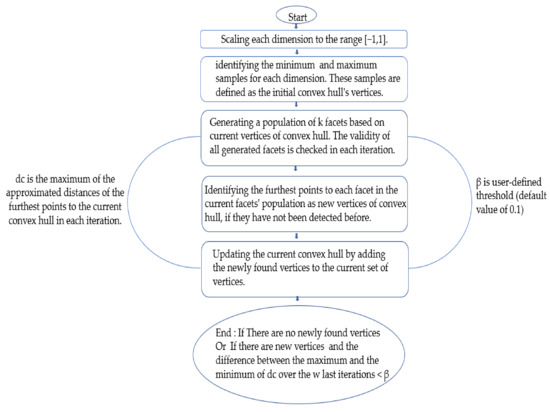
Figure 1. ApproxHull algorithm flowchart. Adapted from reference [62].

It should be noted that before applying ApproxHull, the original dataset is preprocessed. For equal columns (identical features) and duplicated rows (equal samples), rows with non-numerical values and rows with missing values are excluded to reduce the possibility of ApproxHull generating a singular matrix corresponding to a random invalid facet. ApproxHull ensures that all convex hull points from the design data are included in the training set, which is then augmented with samples randomly extracted from the design data to obtain the user-specified number of samples for the training set. The remaining design data are randomly split to the testing and validation sets, according to the user specifications. As a result of this procedure, training, testing, and validation sets are generated.

3.2. Convolutional Neural Network (CNN)

In recent years, convolutional networks have seen a series of successes in classifying large-scale images [60]. Its effectiveness stems from its ability to model nonlinear local dependencies [64,65]. A convolutional neural network architecture is typically made up of three layers: convolutional layer, pooling layer, and fully connected layer. The convolutional layer aims to extract features that represent the inputs. It is made up of many convolution kernels that are used to compute distinct feature maps [66]. Equation (3) describes the feature maps using several distinct kernels:

$$z_{i,j,k}^l=W_k^l{x}_{i,j}^l+b_k^l$$

(3)

where $x_{i,j}^l$ denotes the inputs of the lth layer at location (I, j), $W_k^l$ and $b_k^l$ represent, respectively, the weight vector and bias term of the lth layer and kth filter. Nonlinearities are introduced into CNN via the activation function, which is useful for multi-layer networks to capture nonlinear features. The activation function is given by:

$${\phi }_{i,j,k}^l=\phi \left(z_{i,j,k}^l\right)$$

(4)

The ReLu activation function is used in this work [67].

$$\mathrm{ReLu}\left(x\right)=\max \left(0,x\right)$$

(5)

The pooling layer enables to select and filter the features extracted by the convolutional layer. It intends to achieve shift-invariance by lowering the resolution of the feature maps. The pooling function for each feature map ${\phi }_{:,:,k}^l$ is as follows:

$$y_{i,j,k}^l=\mathrm{pool}\left({\phi }_{m,n,k}^l\right),\forall \left(m,n\right)\in R_{ij}$$

(6)

where $R_{ij}$ denotes a local neighborhood around location (I, j). The max-pooling is used in this work for pooling operation. Its output with stride l and size s is defined by:

y(i) = max x[i × l: i × l + s − 1]

(7)

The fully connected layers seek to conduct high-level reasoning. They connect all neurons of the previous layer to every neuron in the current layer to produce global semantic information. The output is generated by nonlinearly combining the features that have been selected with the fully connected layer.

Training a CNN involves minimizing a suitable loss function. Given a set of input output {($x^{\left(k\right)},y^{\left(k\right)}$), k = [1, $\dots ,K]\}$, where $x^{\left(K\right)}$ denotes the kth input data and $y^{\left(k\right)}$ is the matching target label, assume that θ represents all the CNN parameters and o is the CNN output. The loss function of CNN may be computed as follows:

$$\Gamma =\frac{1}{N}{{\displaystyle \sum }}_{n=1}^N{\ell }(\theta ,y^{\left(n\right)},o)$$

(8)

The best fitting set of parameters may be found by minimizing the loss function. Further information about CNN models can be found in [66]. The trial-and-error procedure was used to tune the CNN hyperparameters. The classification subnetwork CNN architecture proposed with the best hyperparameters values is as follows:

• Input shape (length defined by the appliance data).
• 1D convolutional layer (filters = 32, kernel size = 3, activation = ‘ReLu’).
• 1D convolutional layer (filters = 64, kernel size = 3, activation = ‘ReLu’).
• 1D convolutional layer (filters = 128, kernel size = 3, activation = ‘ReLu’).
• Maxpool layer.
• Fully connected dense layer (number of units = 1024, activation = ’ReLu’).
• Fully connected dense layer (number of units = 1).

3.3. Long Short-Term Memory (LSTM)

LSTM has been introduced by [68] to address both long-term and short-term dependency issues. It is a deep recurrent neural network that uses a feed-forward variation to process sequential data and address vanishing gradient issues. The LSTM design replaces the hidden layer of the conventional neural network units with combined memory cells. It is made up of three gates: an input gate, a forget gate, and an output gate. The state of the memory cell is referred to as a cell state. The LSTM network may add or delete information to the memory cell state via the input gate, output gate, and forget gate. Each gate has a specific purpose that is determined by the current external input and the previous cell’s output. The input gate determines how much the block input will update the cell state. The forget gate determines which information from the prior cell state should be erased and which should be stored. It enables the cell to memorize or forget its prior state, as necessary. The output gate determines which piece of the cell state should be propagated to the output. The block output is then computed by multiplying the filtered current cell state by the output gate. It can enable or prevent the cell state from affecting other neurons. Figure 2 presents the architecture of the LSTM cell. The terms $i_t,f_t,o_t,h_t,c_t$ denote, respectively, the input gate, forget gate, output gate, the output, and the cell state. The symbols σ and tanh represent the sigmoid activation function and the tanh activation function, respectively.

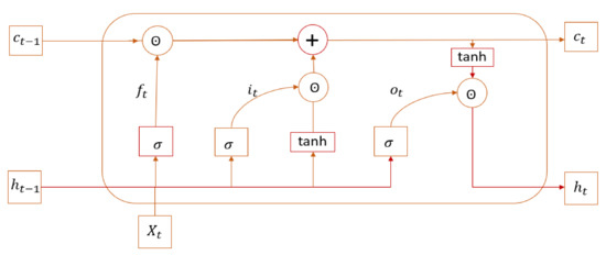
Figure 2. LSTM cell architecture. Adapted from reference [68].

One of the approaches to improve the recurrent neural network models is the usage of bidirectional layers [13]. Indeed, one recurrent neural network reads the input sequence forward, while the other reads it backward. To merge the output from the network’s forward and backward sides, an element-wise sum is employed. The bidirectional LSTM network predicts actual value using both prior and future information, and in this way is an ideal model for the NILM problem [57]. It is made up of three layers: input layer, hidden layer, and output layer. The hidden layer is made up of two unidirectional LSTM layers that have identical architecture and the same input but propagate the data in the opposite direction. The following are the vector formulas defining the forward LSTM layer for the propagation process [69].

$$f_t=\mathsf{\sigma }(W_f.\left[h_{t-1},x_t\right]+b_f)$$

(9)

$$i_t=\mathsf{\sigma }\left(W_i.\left[h_{t-1},x_t\right]+b_i\right)$$

(10)

$$\widehat{c_t}=\tanh \left(W_c.\left[h_{t-1},x_t\right]+b_c\right)$$

(11)

$$c_t=f_t\odot c_{t-1}+i_t\odot \widehat{c_t}$$

(12)

$$o_t=\mathsf{\sigma }\left(W_o.\left[h_{t-1},x_t\right]+b_o\right)$$

(13)

$$\widehat{h_t}=\tanh \left(c_t\right)$$

(14)

$$h_t=o_t\odot \widehat{h_t}$$

(15)

where $\odot$ denotes element-by-element multiplication. $W_f$, $W_i$, $W_c$,$W_o$ and $b_f$, $b_i$, $b_c$, $b_o$ are the weight matrices and bias vectors for forget gate, input gate, cell state, and output gate, respectively, in the forward LSTM layer.

The information propagation mechanism in the backward LSTM layer is described as follows:

$$f_t^{\prime }=\mathsf{\sigma }(W_f^{\prime }.\left[h_{t+1}^{\prime },x_t\right]+b_f^{\prime })$$

(16)

$$i_t^{\prime }=\mathsf{\sigma }\left(W_i^{\prime }.\left[h_{t+1}^{\prime },x_t\right]+b_i^{\prime }\right)$$

(17)

$${\widehat{c}}_t^{\prime }=\tanh \left(W_C^{\prime }.\left[h_{t+1}^{\prime },x_t\right]+b_c^{\prime }\right)$$

(18)

$$c_t^{\prime }=f_t^{\prime }\odot c_{t-1}^{\prime }+i_t^{\prime }\odot {\widehat{c}}_t^{\prime }$$

(19)

$$o_t^{\prime }=\mathsf{\sigma }\left(W_o^{\prime }.\left[h_{t+1}^{\prime },x_t\right]+b_o^{\prime }\right)$$

(20)

$$\widehat{h_t^{\prime }}=\tanh \left(c_t^{\prime }\right)$$

(21)

$$h_t^{\prime }=o_t^{\prime }\odot \widehat{h_t^{\prime }}$$

(22)

where $W_f^{\prime }$, $W_I^{\prime }$, $W_C^{\prime },W_O^{\prime }$ and $b_f^{\prime }$, $b_i^{\prime },b_c^{\prime }$, $b_o^{\prime }$ are the weight matrices and bias vectors for the forget gate, input gate, cell state, and output gate, respectively, in the backward LSTM layer.

The bidirectional LSTM output vector is defined by:

$${\widehat{y}}^b=W_s.\left(h_t\oplus h_t^{\prime }\right)+b_s$$

(23)

where $W_s$ and $b_s$ denote the weight matrix and bias vector of the output layer. The symbol ⊕ denotes vector splicing.

The loss function used is the mean square error (MSE) defined by:

$$\mathrm{MSE}=\frac{1}{N}{\displaystyle \sum }_{i=1}^N{\left({\widehat{y}}_i^b-y_i^b\right)}^2$$

(24)

The best fit of the model is obtained by minimizing the mean square error loss function. For more details about the LSTM model, please refer to [68]. The subnetwork architecture of the regression model with the optimal parameters used is as follows:

• Input shape (length defined by the appliance data).
• Bidirectional LSTM layer (number of hidden units = 32, activation = ‘ReLu’).
• Dropout layer with dropout = 0.3.
• Bidirectional LSTM layer (number of hidden units = 64, activation = ‘ReLu’).
• Dropout layer with dropout = 0.3.
• Bidirectional LSTM layer (number of hidden units = 128, activation = ‘ReLu’).
• Dropout layer with dropout = 0.3.
• Fully connected dense layer (number of units = 1024, activation = ’ReLu’).
• Fully connected dense layer (number of units = 1).

The general framework of the proposed disaggregation architecture is made up of two subnetworks architecture. Each subnetwork is considered as a subtask of the energy disaggregation task [63]. On the one hand, the classification is performed using the CNN architecture. The goal is to detect if the device is ON or OFF. It is assumed that a device is ON when its power consumption exceeds a certain threshold, and it is OFF elsewise. The input of the network is the training data selected using ApproxHull algorithm. The output of the classification subnetwork is the state of the device $s_t^{\left(i\right)}$= {$s_1^{\left(i\right)},\cdots ,$ $s_T^{\left(i\right)}$}, where $s_t^{\left(i\right)}$∈ {0,1} represents the ON-OFF state of device i at time t. On the other hand, the power sequence of the device is estimated using the bidirectional LSTM subnetwork architecture. The usage of recurrent neural networks enables the model to have an accurate estimate of every device’s energy usage while also ensuring the overall network architecture scalability. Assume that ${\widehat{s}}_t^i=f_c^i(X_t$), where $f_c^i$ is the device state classification subnetwork model and $X_t$ is the input. Let ${\widehat{p}}_t^i$ = $f_r^i\left(X_t\right)$, where $f_r^i\mathrm{is}$ the device power sequence estimate regression model. The final disaggregation output is generated by multiplying the classification subnetwork output by the regression subnetwork’s predicted power sequence, defined as:

$${\widehat{y}}_t^{\left(i\right)}={\widehat{s}}_t^i\odot {\widehat{p}}_t^i$$

(25)

where ${\widehat{y}}_t^{\left(i\right)}$ is the disaggregation output of appliance I at time t, and ${\widehat{s}}_t^i$ and ${\widehat{p}}_t^i$ denote, respectively, the output of the classification and regression subnetworks. Figure 3 depicts the full proposed disaggregation model architecture.

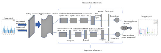
Figure 3. Proposed disaggregation model architecture.

3.4. Dataset

This study makes use of data collected from a detached household, a typical residential house located in Algarve, Portugal. It is equipped with a multitude of electrical appliances. The electric board includes 17 circuits breakers, 16 monophasic and 1 triphasic. A Circutor Wibee [70] measures each circuit breaker, with a sample interval of 1 s. The total aggregate consumption that will be used for the proposed NILM algorithm is measured by a three-phase energy meter from Carlo Gavazzi (EM340) [71]. It measures 45 distinct electric variables in the house sampled at 1 Hz. Table 1 presents the most important devices attached in each phase. Additional electric variables are monitored for each circuit breaker to obtain an approximation of ground truth for each appliance. A total of 198 variables are measured by the Circutor Wibee, including current, voltage, active power, reactive power, apparent power, frequency, power factor, capacitive reactive energy, and inductive reactive energy. Additionally, smart plugs enable the measurement of individual sockets from the same circuit breaker. Currently, three smart plugs are used, allowing monitoring of six additional variables every second, for each smart plug. It should be noted that the measuring equipment are not synchronized, and thus, the acquisition time instants for each meter differ. The house includes a PV installation made up of twenty Sharp NU-AK panels [72]. A Kostal Plenticore Plus inverter [73] is used, controlling also a BYD Battery Box HVH 11.5 [74] with a storage capacity of 11.5 kWh. From the inverter, 47 electrical variables are sampled each minute. An intelligent weather station (IWS) [75], measuring global solar radiation, atmospheric air temperature, and relative humidity, and a few self-powered wireless sensors (SPWS) [76] are employed for monitoring climate variables inside the house. The climate variables include relative humidity, air temperature, wall temperature, and movement. The transfer of data from/to the measurement appliances is handled by gateways and a technical network. The data is accessed through a wireless IP network using the Modbus IP protocol. An IoT platform was set up. For further details about the whole data acquisition system please refer to [77].

Table 1. Description of the devices in the house. LFL: linear fluorescent lamp, CFL: compact fluorescent lamp, LL: LED lamp, AC: air conditioner, TV: television, IL: incandescent lamp.

Phase	Devices
1	Security alarm, LFL_1, CFL_1, CFL_2, LL_1, LL_2, CFL_3, CFL_4, running machine, clothes iron, electric air heater_1, hair dryer_1, AC_1, AC_2, AC_3, CFL_5, CFL_6, LL_3, CFL_24, CFL_7, broadband router_1, electric air heater_2, electric air heater_3, immersion heater, aquarium pump, CFL_8, desktop computer, laptop computer_1, laptop computer_2, TV_1, audio system_1, printer, broadband router_2, and burner stove_1.
2	Swimming pool pump, IL_1, IL_2, LFL_2, LL_4, LL_5, LFL_4, hair dryer_2, LL_6, motor_1, motor_2, washing machine, electric water heating, broadband router_3, dryer, fridge freezer_1, coffee maker, toaster, food processor, small cooking appliance, TV_2, fridge freezer_3, freezer, LL_13, CFL_9, CFL_10, CFL_11, CFL_12, LFL_3, CFL_13, CFL_14, LL_7, and oven.
3	LL_8, CFL_15, CFL_16, LL_9, LL_10, LL_11, LL_12, CFL_17, CFL_18, CFL_19, CFL_20, CFL_21, CFL_22, AC_4, dish washer, microwave, fryer, kettle, CFL_23, TV_3, audio system_2, set top box, AC_5, and burner stove_2.

3.5. Evaluation Metrics

The proposed approach is based on both the detection of the state of appliances and power estimations. Therefore, it requires the use of both classification and estimation accuracy metrics. The most pertinent evaluation metrics were considered with the objective of reflecting the methodology’s efficiency in both recognizing the activation state and predicting the energy use.

The classification metrics used are defined as follows [78,79]:

$$\mathrm{Recall}=\frac{\mathrm{TP}}{\mathrm{TP}+\mathrm{FN}}$$

(26)

$$\mathrm{Precision}=\frac{\mathrm{TP}}{\mathrm{TP}+\mathrm{FP}}$$

(27)

$$\mathrm{F}1=2\times \frac{\mathrm{Precision}\times \mathrm{Recall}}{\mathrm{Precision}+\mathrm{Recall}}$$

(28)

where TP, FP, and FN denote, respectively, the number of true positives (actual = ON, predicted = ON), false positives (actual = OFF, predicted = ON), and false negatives (actual = ON, predicted = OFF).

The energy estimation metrics used are mean absolute error (MAE), signal aggregate error (SAE), and estimation accuracy (EA). They are described as follows [18,57]:

$${\mathrm{MAE}}^{\left(i\right)}=\frac{{{\displaystyle \sum }}_{t=1}^N\left|y_t^{\left(i\right)}-{\widehat{y}}_t^{\left(i\right)}\right|}{N}$$

(29)

$${\mathrm{SAE}}^{\left(i\right)}=\frac{\left|{\underset{·}{\overset{^}{\mathrm{E}}}}^{\left(i\right)}-E^{\left(i\right)}\right|}{E^{\left(i\right)}}$$

(30)

$${\mathrm{EA}}^{\left(i\right)}=1-\frac{{{\displaystyle \sum }}_1^N\left|y_t^{\left(i\right)}-{\widehat{y}}_t^{\left(i\right)}\right|}{2\times {{\displaystyle \sum }}_{t=1}^N{y}_t^{\left(i\right)}}$$

(31)

where N denotes the number of load data values, $y_t^{\left(i\right)}$ is the ground truth power values of appliance i at time t, ${\widehat{y}}_t^{\left(i\right)}$ is the predicted power values of appliance i at time t, ${\underset{·}{\overset{^}{\mathrm{E}}}}^{\left(i\right)}$ is the total predicted energy, and $E^{\left(i\right)}$ is total ground truth energy for appliance i.

4. Results and Discussion

4.1. Data Pre-Processing

The data were collected for several months from the house described in Section 3.4. In this study, only four weeks of data are considered representing, however, around 1.5 million samples for each device. The aggregated active and reactive powers measured by EM340 for phase 2 are extracted. For each instant of time, a sliding window of 20 variables (10 active and 10 reactive lagged power values) is constructed. These data, together with the label (appliance on/off) if a classification is sought, or the current active power, if a prediction is desired, are fed to the ApproxHull algorithm. To evaluate the proposed approach, four popular appliances for evaluating NILM algorithms are considered. These four devices are within the range of the major consumers in the case study house. They are the washing machine, fridge, swimming pool pump, and electric water heater. The ground truth active power sequence for each appliance is determined manually using the Circutor Wibee measurements and smart plugs data. The ON-OFF status of each appliance is determined using a similar approach to that used in NILMTK [80]. The appliance is considered ON when its consumed power exceeds a defined threshold value for a minimum time threshold. Indeed, for certain multistate appliances where energy consumption can fall below the threshold value for brief periods of time without being switched off, a minimum time threshold is defined during which the power supply is kept below the threshold. The appliance is assumed to be OFF if the time duration where the power is below the power threshold is higher than the minimum time threshold defined. Furthermore, the ON state is obtained from samples that are strictly consecutive above a predefined threshold, where sequences of data smaller than the predefined minimum time threshold are eliminated. Table 2 summarizes the parameters used to generate the device labels.

Table 2. Parameters used to generate appliance status.

Appliances	Max Power (W)	Power Threshold (W)	Time Threshold (s)
Washing machine	2500	20	3
Electric water heating	1700	1500	3
Swimming pool pump	1200	500	3600
Fridge	200	50	60

Table 3 presents some statistics about the number of activations, the maximum and the average ON duration, and the total active energy consumed for each device over the considered data period.

Table 3. Appliance statistics.

Appliances	ON Duration (s)		Activations	Energy (kWh)
	Max	Average
Washing machine	8696	2550	17	9.5
Electric water heating	10,169	561	663	122.9
Swimming pool pump	25,202	24,985	28	159.1
Fridge	7045	2100	708	36.1

The ApproxHull algorithm described in Section 3.1 is applied to the overall dataset (four weeks of data sampled every second, consisting of 2,419,200 samples), to generate training, testing, and validation sets for each appliance. One dataset is created for each appliance. First, the convex points representing the whole input range in which the model is supposed to be employed are generated. Then, all the convex points found are included in the training set for each appliance dataset. Following that, the remaining samples are randomly distributed throughout the balance of the training, testing, and validation sets, in the ratios of 60%, 20%, and 20%, respectively. Table 4 presents the average number of vertices and the size of the training, testing, and validation datasets for each appliance.

Table 4. Size of training, testing, and validation sets.

Appliances	CH Vertices	Training Set	Testing Set	Validation Set
Washing machine	170	1,451,513	483,839	483,837
Electric water heating	118	1,375,956	458,652	458,652
Swimming pool pump	109	1,375,956	458,652	458,652
Fridge	106	1,375,956	458,652	458,652

4.2. Training and Testing

One model is trained for each appliance. The experiments were conducted using data from 1 March 2021 to 28 March 2021 for the washing machine and from 2 June 2021 to 30 June 2021 for the other appliances. A hyperparameter tweaking was conducted to obtain the optimum hyperparameter settings. The network parameters are obtained using Adam optimization method [81] utilizing a learning rate of 5 × 10⁻⁵ and a batch size of 512. The binary cross entropy loss function was used for the classification subnetwork and the mean square error loss function for the regression subnetwork. The full architecture loss function is the result of combining the loss functions of the two subnetworks. Early stopping was used to avoid overfitting [82]. It is also called implicit regularization since it interrupts the training when the error on the validation set increases. Table 5 and Table 6 present the summary of results obtained in the test dataset in terms of state identification and estimation of energy of each appliance without ApproxHull and with ApproxHull, respectively.

Table 5. Performance’s evaluation results without ApproxHull: mean absolute error (MAE), signal aggregate error (SAE), and estimation accuracy (EA).

Appliance	TP	TN	FP	FN	Recall	Precision	F1	MAE (W)	SAE	EA
Washing machine	9872	469,495	3959	511	0.95	0.71	0.81	8.90	0.46	0.66
Electric water heating	74,424	380,307	3107	814	0.98	0.95	0.97	18.5	0.007	0.96
Swimming pool pump	126,772	331,301	379	200	0.99	0.99	0.99	6.6	0.016	0.98
Fridge	291,218	105,227	28,595	33612	0.89	0.91	0.90	17.5	0.17	0.83

Table 6. Performance’s evaluation results with ApproxHull: mean absolute error (MAE), signal aggregate error (SAE), and estimation accuracy (EA).

Appliance	TP	TN	FP	FN	Recall	Precision	F1	MAE (W)	SAE	EA
Washing machine	13,034	469,737	547	519	0.96	0.96	0.96	1.64	0.05	0.93
Electric water heating	55,157	403,053	158	284	0.99	0.99	0.99	5.0	0.007	0.98
Swimming pool pump	134,803	323,699	64	86	0.99	0.99	0.99	4.92	0.002	0.98
Fridge	326,212	99,553	25,862	7025	0.97	0.92	0.95	12.72	0.09	0.88

The results demonstrate the model’s effectiveness in recognizing and estimating the energy of each device. The proposed ApproxHull data selection approach has significantly improved the model’s performance when compared to the model without ApproxHull, particularly for multistate devices (washing machine and fridge) that have a complex signature behavior and, therefore, are difficult to identify (worse F1 value).

Indeed, the mean absolute error for the washing machine and fridge have been lowered, respectively, by 81% and 27% with the ApproxHull data selection. For the electric water heater and swimming pool pump, the mean absolute error was reduced by 73% and 25%, respectively. The F1 score of the washing machine and fridge were improved by 18% and 5% using ApproxHull data selection.

Regarding the estimation accuracy (EA), there is an improvement of 40% for the washing machine and 6% for the fridge using ApproxHull data selection. Due to their basic architecture, the electric water heater and swimming pool pump could be disaggregated with good performance. Nevertheless, by employing ApproxHull, performance presented slightly higher values both in terms of estimation accuracy and F1. Figure 4 and Figure 5 depict the comparison of both F1 score and estimation accuracy without ApproxHull and when ApproxHull data selection is employed for all the devices considered in the experiment.

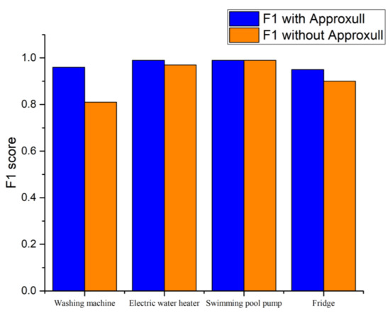
Figure 4. F1 score comparison without and with ApproxHull data selection algorithm.

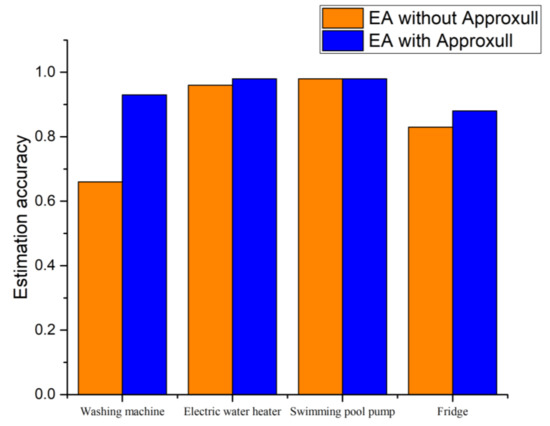
Figure 5. Estimation Accuracy (EA) comparison without and with ApproxHull data selection algorithm.

Despite the complex architecture of multi-state devices, the proposed data selection approach enables a more accurate identification and estimation of each device’s consumption. Some examples of disaggregation outputs are presented in Figure 6, Figure 7, Figure 8 and Figure 9. Figure 6 shows the estimated active power consumption versus the ground truth active power of the washing machine as well as the aggregated active power. Figure 7 presents the estimated active power of the fridge compared to its ground truth. The aggregated power can be seen in Figure 8 and Figure 9. Figure 8 and Figure 9 depict the aggregate active power, the ground truth, and the estimated active power for the electric water heater and swimming pool pump, respectively.

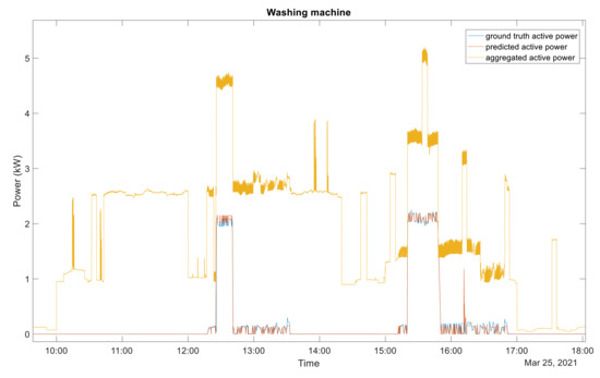
Figure 6. Disaggregation output of the washing machine. Blue, ground truth active power; red, predictive active power; yellow, aggregate active power.

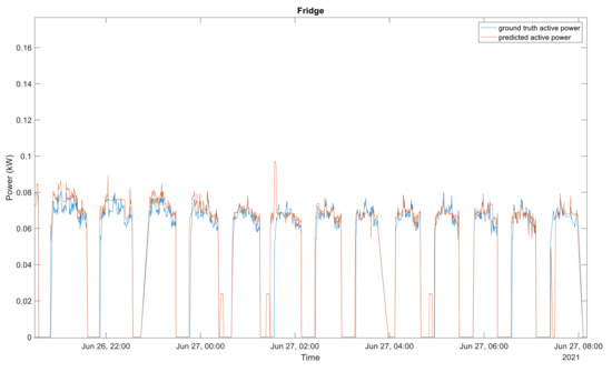
Figure 7. Disaggregation output of the fridge. Blue, ground truth active power; red, predictive active power.

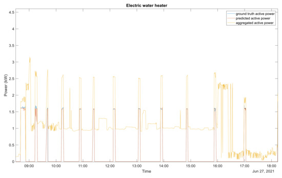
Figure 8. Disaggregation output of the electric water heater. Blue, ground truth active power; red, predictive active power; yellow, aggregate active power.

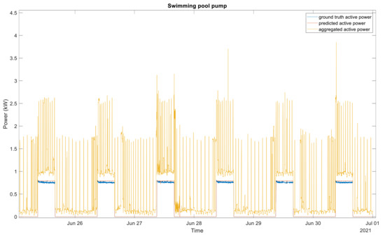
Figure 9. Disaggregation output of the swimming pool pump. Blue, ground truth active power; red, predictive active power; yellow, aggregate active power.

As it can be seen in Figure 6, Figure 7, Figure 8 and Figure 9, there is a very good agreement between the estimated active power and the ground truth active for all four appliances considered in the experiment. The estimated power consumption signals are very close to the ground truth. It should also be mentioned that each of these devices presented very satisfactory performances.

To validate the reproducibility of the experiment, a five-fold cross validation was used. As in the original experiment, 80% of the data was used for training and 20% for testing; the design data was partitioned into five mutually exclusive subsets of equal size, with one subset being utilized for testing and the remaining four being used to estimate the parameters and compute the model’s accuracy. This process is performed k times by circularly alternating the test subset. Table 7 presents the results of the five-cross-validation for the washing machine and fridge in term of F1 score.

Table 7. F1 score using cross validation.

Washing Machine	0.963	0.961	0.959	0.958	0.959
Fridge	0.944	0.938	0.950	0.934	0.947

4.3. Comparison with Other State-of-the-Art Techniques

As highlighted in [14,31] the direct comparison of NILM methods is not easy because of the ambiguity on the evaluation metrics which depends on data and on the context of experiments. The approach proposed in this paper is based on a private house data sampled at a low frequency of 1 Hz. It employs past active and reactive powers as inputs. However, in most of the existing low frequency public dataset only active power measurements are available [53,54]. Thus, an accurate qualitative comparison of methods with different datasets is not possible. However, as an illustration, a comparison was conducted. Table 8 presents the comparison of the proposed NILM approach to state of art NILM methods for washing machine.

Table 8. Comparison results with existing non-intrusive load monitoring methods for washing machine.

Method	Recall	Precision	F1	MAE (W)	SAE	EA
Online-NILM [42]	1	0.60	0.70	118.11	-	-
MFS-LSTM [57]	-	-	0.76	14.42	0.51	0.74
CNN [83]	0.78	0.20	0.32	18.38	-	-
LDwA [61]	-	-	0.69	11.17	-	-
CNN [60]	0.98	0.87	0.92	-	-	0.92
TP-NILM [18]	0.86	0.87	0.86	8.31	0.01	-
Proposed	0.96	0.96	0.96	1.64	0.05	0.93

The performances comparison of the fridge to the state-of-the-art methods is presented in Table 9.

Table 9. Comparison results with existing non-intrusive load monitoring methods for the fridge.

Method	Recall	Precision	F1	MAE (W)	SAE	EA
Online-NILM [42]	0.73	0.87	0.79	4.34	-	-
MFS-LSTM [57]	-	-	0.87	19.60	0.46	0.76
CNN [83]	0.97	0.80	0.88	7.90	-	-
LDwA [61]	-	-	0.86	19.81	-	-
TP-NILM [18]	0.89	0.85	0.87	17.03	−0.05	-
Proposed	0.97	0.92	0.95	12.72	0.09	0.88

The results presented in Table 8 and Table 9 show that the proposed approach is very effective in identifying the states of the devices and in estimating the energy consumed by each device. Fridge and washing machine are very common multi-state appliances for testing NILM algorithms. For the washing machine, the proposed approach achieves the best results in terms of precision (96%), F1 score (96%), mean absolute error (1.64 W), and estimation accuracy (93%). However, it obtained a slightly worse recall (96%) than CNN (98%) presented in [60] and Online-NILM (100%) proposed in [42].

For the fridge, the proposed approach consistently outperforms state-of-the-art methods in terms of recall (97%), precision (92%), F1 score (95%), and estimation accuracy (88%). Conversely, it had a slightly worse mean absolute error of 12.72 W compared to the Online-NILM 4.34 W presented in [42]. The overall results demonstrate that, when compared to state-of-the-art algorithms, the proposed approach effectively disaggregates target devices with higher power estimation accuracy and a superior F1 score.

5. Conclusions

This paper proposes an NILM framework based on low frequency power data using a convex hull data selection approach and a hybrid deep learning architecture. Data were collected in a private house in Algarve, Portugal. The input of the model is a sliding window of active and reactive power values sampled at 1 Hz.

As a primary step, data selection using a randomized approximation convex hull is conducted. It is based on the selection of the most informative vertices from the real convex hull. Then, a hybrid deep learning model is designed by combining two sub-network models. It is built by combining a classification subnetwork model based on convolutional neural networks with a regression subnetwork model based on bidirectional long short-term memory neural networks.

The output of the classification subnetwork is the sequence of states of the devices, whereas the output of the regression subnetwork is the power sequence of the target device at each time instant. In fact, the regression subnetwork tends to predict irrelevant powers that do not belong to the target device. The use of a classification subnetwork enables the detection of the device’s ON/OFF state and, therefore, the elimination of any prediction that does not belong to the target device under analysis. The model’s output is generated by merging the results of two subnetworks.

The obtained results demonstrated that the use of the ApproxHull data selection approach significantly enhances the performance of the designed model particularly for multi-state devices. Moreover, the results of the test showed that the proposed approach accurately disaggregates target devices with higher power estimation accuracy and a superior F1 score than state-of-the-art approaches.

ApproxHull data selection may be used for both offline training and online modeling. Future work will focus on the implementation of the proposed approach for online non-intrusive load monitoring application in home energy management systems.

References

- Dong, K.; Dong, X.; Jiang, Q. How renewable energy consumption lower global CO2 emissions? Evidence from countries with different income levels. World Econ. 2020, 43, 1665–1698. [Google Scholar] [CrossRef]
- IEA Portugal 2021, IEA, Paris. Available online: https://www.iea.org/reports/portugal-2021 (accessed on 3 December 2021).
- Zhang, M.; Zhang, K.; Hu, W.; Zhu, B.; Wang, P.; Wei, Y.M. Exploring the climatic impacts on residential electricity consumption in Jiangsu, China. Energy Policy 2020, 140, 111398. [Google Scholar] [CrossRef]
- Bertoldi, P.; Economidou, M.; Palermo, V.; Boza-Kiss, B.; Todeschi, V. How to finance energy renovation of residential buildings: Review of current and emerging financing instruments in the EU. Wiley Interdiscip. Rev. Energy Environ. 2021, 10, e384. [Google Scholar] [CrossRef]
- Lopes, M.A.R.; Antunes, C.H.; Reis, A.; Martins, N. Estimating energy savings from behaviours using building performance simulations. Build. Res. Inf. 2017, 45, 303–319. [Google Scholar] [CrossRef]
- Xu, X.; Xiao, B.; Li, C.Z. Critical factors of electricity consumption in residential buildings: An analysis from the point of occupant characteristics view. J. Clean. Prod. 2020, 256, 120423. [Google Scholar] [CrossRef]
- Tzeiranaki, S.T.; Bertoldi, P.; Diluiso, F.; Castellazzi, L.; Economidou, M.; Labanca, N.; Serrenho, T.R.; Zangheri, P. Analysis of the EU Residential Energy Consumption: Trends and Determinants. Energies 2019, 12, 1065. [Google Scholar] [CrossRef] [Green Version]
- Balezentis, T. Shrinking ageing population and other drivers of energy consumption and CO2 emission in the residential sector: A case from Eastern Europe. Energy Policy 2020, 140, 111433. [Google Scholar] [CrossRef]
- Mattinen, M.K.; Heljo, J.; Vihola, J.; Kurvinen, A.; Lehtoranta, S.; Nissinen, A. Modeling and visualization of residential sector energy consumption and greenhouse gas emissions. J. Clean. Prod. 2014, 81, 70–80. [Google Scholar] [CrossRef]
- IEA Appliances and Equipment, IEA, Paris. Available online: https://www.iea.org/reports/appliances-and-equipment (accessed on 14 December 2021).
- Ruano, A.; Hernandez, A.; Ureña, J.; Ruano, M.; Garcia, J. NILM Techniques for Intelligent Home Energy Management and Ambient Assisted Living: A Review. Energies 2019, 12, 2203. [Google Scholar] [CrossRef] [Green Version]
- Marangoni, G.; Tavoni, M. Real-time feedback on electricity consumption: Evidence from a field experiment in Italy. Energy Effic. 2021, 14, 1–17. [Google Scholar] [CrossRef]
- Kelly, J.; Knottenbelt, W. Neural NILM: Deep Neural Networks Applied to Energy Disaggregation. In Proceedings of the 2nd ACM International Conference on Embedded Systems for Energy-Efficient Built Environments, ACM, Seoul, Korea, 4–5 November 2015; pp. 55–64. [Google Scholar] [CrossRef] [Green Version]
- Laouali, I.H.; Qassemi, H.; Marzouq, M.; Ruano, A.; Bennani, S.D.; El Fadili, H. A survey on computational intelligence techniques for non intrusive load monitoring. In Proceedings of the 2020 IEEE 2nd International Conference on Electronics, Control, Optimization and Computer Science, ICECOCS 2020, IEEE, Kenitra, Marroco, 2 December 2020. [Google Scholar]
- Zoha, A.; Gluhak, A.; Imran, M.A.; Rajasegarar, S. Non-intrusive Load Monitoring approaches for disaggregated energy sensing: A survey. Sensors 2012, 12, 16838–16866. [Google Scholar] [CrossRef] [Green Version]
- Abubakar, I.; Khalid, S.N.; Mustafa, M.W.; Shareef, H.; Mustapha, M. Application of load monitoring in appliances’ energy management—A review. Renew. Sustain. Energy Rev. 2017, 67, 235–245. [Google Scholar] [CrossRef]
- Saha, D.; Bhattacharjee, A.; Chowdhury, D.; Hossain, E.; Islam, M.M. Comprehensive NILM Framework: Device Type Classification and Device Activity Status Monitoring Using Capsule Network. IEEE Access 2020, 8, 179995–180009. [Google Scholar] [CrossRef]
- Massidda, L.; Marrocu, M.; Manca, S. Non-intrusive load disaggregation by convolutional neural network and multilabel classification. Appl. Sci. 2020, 10, 1454. [Google Scholar] [CrossRef] [Green Version]
- Puente, C.; Palacios, R.; González-Arechavala, Y.; Sánchez-Úbeda, E.F. Non-intrusive load monitoring (NILM) for energy disaggregation using soft computing techniques. Energies 2020, 13, 3117. [Google Scholar] [CrossRef]
- Esa, N.F.; Abdullah, M.P.; Hassan, M.Y. A review disaggregation method in Non-intrusive Appliance Load Monitoring. Renew. Sustain. Energy Rev. 2016, 66, 163–173. [Google Scholar] [CrossRef]
- Hart, G.W. Nonintrusive Appliance Load Monitoring. Proc. IEEE 1992, 80, 1870–1891. [Google Scholar] [CrossRef]
- Lindahl, P.A.; Green, D.H.; Bredariol, G.; Aboulian, A.; Donnal, J.S.; Leeb, S.B. Shipboard Fault Detection Through Nonintrusive Load Monitoring: A Case Study. IEEE Sens. J. 2018, 18, 8986–8995. [Google Scholar] [CrossRef]
- Hernández, Á.; Ruano, A.; Ureña, J.; Ruano, M.G.; Garcia, J.J. Applications of NILM Techniques to Energy Management and Assisted Living. FAC-PapersOnLine 2020, 52, 164–171. [Google Scholar] [CrossRef]
- De Baets, L.; Develder, C.; Dhaene, T.; Deschrijver, D. Detection of unidentified appliances in non-intrusive load monitoring using siamese neural networks. Int. J. Electr. Power Energy Syst. 2019, 104, 645–653. [Google Scholar] [CrossRef]
- Liu, Y.; Wang, X.; You, W. Non-intrusive Load Monitoring by Voltage-Current Trajectory Enabled Transfer Learning. IEEE Trans. Smart Grid 2018, 10, 5609–5619. [Google Scholar] [CrossRef]
- Singh, S.; Majumdar, A. Deep sparse coding for non-intrusive load monitoring. IEEE Trans. Smart Grid 2018, 9, 4669–4678. [Google Scholar] [CrossRef] [Green Version]
- Çavdar, I.H.; Faryad, V. New design of a supervised energy disaggregation model based on the deep neural network for a smart grid. Energies 2019, 12, 1217. [Google Scholar] [CrossRef] [Green Version]
- Devlin, M.A.; Hayes, B.P. Non-Intrusive Load Monitoring and Classification of Activities of Daily Living using Residential Smart Meter Data. IEEE Trans. Consum. Electron. 2019, 65, 339–348. [Google Scholar] [CrossRef]
- Fagiani, M.; Bonfigli, R.; Principi, E.; Squartini, S.; Mandolini, L. A non-intrusive load monitoring algorithm based on non-uniform sampling of power data and deep neural networks. Energies 2019, 12, 1371. [Google Scholar] [CrossRef] [Green Version]
- Liu, Q.; Kamoto, K.M.; Liu, X.; Sun, M.; Linge, N. Low-Complexity Non-Intrusive Load Monitoring Using Unsupervised Learning and Generalized Appliance Models. IEEE Trans. Consum. Electron. 2019, 65, 28–37. [Google Scholar] [CrossRef]
- Zeifman, M.; Roth, K. Nonintrusive appliance load monitoring: Review and outlook. IEEE Trans. Consum. Electron. 2011, 57, 76–84. [Google Scholar] [CrossRef]
- Hart, G.W. Prototype Nonintrusive Appliance load Monitor: Progress Report 2; MIT Energy Laboratory: Concord, MA, USA, 1985. [Google Scholar]
- Huber, P.; Calatroni, A.; Rumsch, A.; Paice, A. Review on deep neural networks applied to low-frequency nilm. Energies 2021, 14, 2390. [Google Scholar] [CrossRef]
- Makonin, S.; Popowich, F.; Bajic, I.V.; Gill, B.; Bartram, L. Exploiting HMM Sparsity to Perform Online Real-Time Nonintrusive Load Monitoring. IEEE Trans. Smart Grid 2016, 7, 2575–2585. [Google Scholar] [CrossRef]
- Bonfigli, R.; Principi, E.; Fagiani, M.; Severini, M.; Squartini, S.; Piazza, F. Non-intrusive load monitoring by using active and reactive power in additive Factorial Hidden Markov Models. Appl. Energy 2017, 208, 1590–1607. [Google Scholar] [CrossRef]
- Zoha, A.; Gluhak, A.; Nati, M.; Imran, M.A. Low-power appliance monitoring using Factorial Hidden Markov Models. In Proceedings of the 2013 IEEE 8th International Conference on Intelligent Sensors, Sensor Networks and Information Processing, ISSNIP 2013, Melbourne, VIC, Australia, 2–5 April 2013. [Google Scholar]
- Kolter, J.Z.; Jaakkola, T. Approximate inference in additive factorial HMMs with application to energy disaggregation. J. Mach. Learn. Res 2012, 22, 1472–1482. [Google Scholar]
- Zia, T.; Bruckner, D.; Zaidi, A. A hidden Markov model based procedure for identifying household electric loads. In Proceedings of the 37th Annual Conference of the IEEE Industrial Electronics Society, Melbourne, VIC, Australia, 7–10 November 2011; pp. 3218–3223. [Google Scholar] [CrossRef]
- Mauch, L.; Yang, B. A New Approach for Supervised Power Disaggregation by Using a Deep Recurrent LSTM. In Proceedings of the 2015 IEEE Global Conference on Signal and Information Processing (GlobalSIP), Orlando, FL, USA, 13–16 December 2015; pp. 63–67. [Google Scholar]
- Kim, H.; Marwah, M.; Arlitt, M.; Lyon, G.; Han, J. Unsupervised Disaggregation of Low Frequency Power Measurements. In Proceedings of the 2011 SIAM International Conference on Data Mining, Mesa, AZ, USA, 28–30 April 2011; Society for Industrial and Applied Mathematics: Philadelphia, PA, USA, 2011; pp. 747–758. [Google Scholar]
- Parson, O.; Ghosh, S.; Weal, M.; Rogers, A. Non-Intrusive Load Monitoring Using Prior Models of General Appliance Types. In Proceedings of the Twenty-Sixth AAAI Conference on Artificial Intelligence, Toronto, ON, Canada, 22–26 July 2012; Elsevier: Amsterdam, The Netherlands, 2012; Volume 217, pp. 356–362. [Google Scholar]
- Mengistu, M.A.; Girmay, A.A.; Camarda, C.; Acquaviva, A.; Patti, E. A Cloud-based On-line Disaggregation Algorithm for Home Appliance Loads. IEEE Trans. Smart Grid 2018, 3053, 1–10. [Google Scholar] [CrossRef]
- Figueiredo, M.B.; De Almeida, A.; Ribeiro, B. An experimental study on electrical signature identification of non-intrusive load monitoring (NILM) systems. Lect. Notes Comput. Sci. 2011, 6594, 31–40. [Google Scholar] [CrossRef]
- Lin, Y.H.; Tsai, M.S.; Chen, C.S. Applications of fuzzy classification with fuzzy c-means clustering and optimization strategies for load identification in NILM systems. In Proceedings of the 2011 IEEE International Conference on Fuzzy Systems (FUZZ-IEEE 2011), Taipei, Taiwan, 27–30 June 2011; pp. 859–866. [Google Scholar] [CrossRef]
- Moradzadeh, A.; Zeinal-Kheiri, S.; Mohammadi-Ivatloo, B.; Abapour, M.; Anvari-Moghaddam, A. Support vector machine-assisted improvement residential load disaggregation. In Proceedings of the 2020 28th Iranian Conference on Electrical Engineering (ICEE), Tabriz, Iran, 4–6 August 2020; pp. 1–6. [Google Scholar] [CrossRef]
- Le, T.T.H.; Kim, H. Non-intrusive load monitoring based on novel transient signal in household appliances with low sampling rate. Energies 2018, 11, 3409. [Google Scholar] [CrossRef] [Green Version]
- Liu, H. Non-Intrusive Load Monitoring: Theory, Technologies and Applications; Springer: Berlin/Heidelberg, Germany, 2019; ISBN 9789811518607. [Google Scholar]
- Giri, S.; Bergés, M.; Rowe, A. Towards automated appliance recognition using an EMF sensor in NILM platforms. Adv. Eng. Inform. 2013, 27, 477–485. [Google Scholar] [CrossRef]
- Azad, S.A.; Ali, A.B.M.S.; Wolfs, P. Identification of typical load profiles using K-means clustering algorithm. In Proceedings of the Asia-Pacific World Congress on Computer Science and Engineering, Nadi, Fiji, 4–5 November 2014; pp. 1–6. [Google Scholar] [CrossRef]
- Zhang, B.; Zhao, S.; Shi, Q.; Zhang, R. Low-rate non-intrusive appliance load monitoring based on graph signal processing. In Proceedings of the 2019 International Conference on Security, Pattern Analysis, and Cybernetics (SPAC), Guangzhou, China, 20–23 December 2019; pp. 11–16. [Google Scholar] [CrossRef]
- He, K.; Stankovic, L.; Liao, J.; Stankovic, V. Non-Intrusive Load Disaggregation Using Graph Signal Processing. IEEE Trans. Smart Grid 2018, 9, 1739–1747. [Google Scholar] [CrossRef] [Green Version]
- Zhang, C.; Zhong, M.; Wang, Z.; Goddard, N.; Sutton, C. Sequence-to-point learning with neural networks for non-intrusive load monitoring. In Proceedings of the Thirty-Second AAAI Conference on Artificial Intelligence, New Orleans, LA, USA, 2–7 February 2018; pp. 2604–2611. [Google Scholar]
- Kolter, J.Z.; Johnson, M.J. REDD: A Public Data Set for Energy Disaggregation Research. In Proceedings of the SustKDD Workshop on Data Mining Applications in Sustainability, San Diego, CA, USA, 21–24 August 2011. [Google Scholar]
- Kelly, J.; Knottenbelt, W. The UK-DALE dataset, domestic appliance-level electricity demand and whole-house demand from five UK homes. Sci. Data 2015, 2, 150007. [Google Scholar] [CrossRef] [Green Version]
- Zhou, X.; Li, S.; Liu, C.; Zhu, H.; Dong, N.; Xiao, T. Non-Intrusive Load Monitoring Using a CNN-LSTM-RF Model Considering Label Correlation and Class-Imbalance. IEEE Access 2021, 9, 84306–84315. [Google Scholar] [CrossRef]
- Pecan Street Inc. Available online: https://dataport.pecanstreet.org/ (accessed on 14 December 2021).
- Rafiq, H.; Shi, X.; Zhang, H.; Li, H.; Ochani, M.K. A deep recurrent neural network for non-intrusive load monitoring based on multi-feature input space and post-processing. Energies 2020, 13, 2195. [Google Scholar] [CrossRef]
- Beckel, C.; Kleiminger, W.; Cicchetti, R.; Staake, T.; Santini, S. The ECO data set and the performance of non-intrusive load monitoring algorithms. In Proceedings of the 1st ACM Conference on Embedded Systems for Energy-Efficient Buildings, BuildSys’14, Memphis, TN, USA, 3–6 November 2014. [Google Scholar]
- Rafiq, H.; Shi, X.; Zhang, H.; Li, H.; Ochani, M.K.; Shah, A.A. Generalizability Improvement of Deep System Using Data Augmentation. IEEE Trans. Smart Grid 2021, 12, 3265–3277. [Google Scholar] [CrossRef]
- Kong, W.; Dong, Z.Y.; Wang, B.; Zhao, J.; Huang, J. A practical solution for non-intrusive type II load monitoring based on deep learning and post-processing. IEEE Trans. Smart Gridw 2020, 11, 148–160. [Google Scholar] [CrossRef]
- Piccialli, V.; Sudoso, A.M. Improving Non-Intrusive Load Disaggregation through an Attention-Based Deep Neural Network. Energies 2021, 14, 847. [Google Scholar] [CrossRef]
- Khosravani, H.R.; Ruano, A.E.; Ferreira, P.M. A convex hull-based data selection method for data driven models. Appl. Soft Comput. J. 2016, 47, 515–533. [Google Scholar] [CrossRef]
- Shin, C.; Joo, S.; Yim, J.; Lee, H.; Moon, T.; Rhee, W. Subtask gated networks for non-intrusive load monitoring. In Proceedings of the Thirty-Third AAAI Conference on Artificial Intelligence and Thirty-First Innovative Applications of Artificial Intelligence Conference and Ninth AAAI Symposium on Educational Advances in Artificial Intelligence, Honolulu, HI, USA, 27 January–1 February 2019; pp. 1150–1157. [Google Scholar] [CrossRef]
- Krizhevsky, A.; Sutskever, I.; Hinton, G.E. ImageNet Classification with Deep Convolutional Neural Networks. Proc. Adv. Neural Inf. Process. Syst. 2012, 25, 1097–1105. [Google Scholar] [CrossRef]
- Russakovsky, O.; Deng, J.; Su, H.; Krause, J.; Satheesh, S.; Ma, S.; Huang, Z.; Karpathy, A.; Khosla, A.; Bernstein, M.; et al. ImageNet Large Scale Visual Recognition Challenge. Int. J. Comput. Vis. 2015, 115, 211–252. [Google Scholar] [CrossRef] [Green Version]
- Gu, J.; Wang, Z.; Kuen, J.; Ma, L.; Shahroudy, A.; Shuai, B.; Liu, T.; Wang, X.; Wang, G.; Cai, J.; et al. Recent advances in convolutional neural networks. Pattern Recognit. 2018, 77, 354–377. [Google Scholar] [CrossRef] [Green Version]
- Nair, V.; Hinton, G.E. Rectified Linear Units Improve Restricted Boltzmann Machines. Available online: https://www.cs.toronto.edu/~fritz/absps/reluICML.pdf (accessed on 10 December 2021).
- Hochreiter, S. Long Short-Term Memory. Neural Comput. 1997, 1780, 1735–1780. [Google Scholar] [CrossRef]
- Jiao, M.; Wang, D. The Savitzky-Golay filter based bidirectional long short-term memory network for SOC estimation. Int. J. Energy Res. 2021, 45, 19467–19480. [Google Scholar] [CrossRef]
- Circutor: Consumption Analyzers. Available online: http://circutor.com/en/products/measurement-and-control/fixed-power-analyzers/consumption-analyzers/wibeee-series-detail (accessed on 20 August 2021).
- Gavazzi, C. Automation Company: EM340 Utilises Touchscreen Technology. Available online: https://www.carlogavazzi.co.uk/blog/carlo-gavazzi-energy-solutions/em340-utilises-touchscreen-technology (accessed on 14 December 2021).
- Sharp NU-AK PV Panels. Available online: https://www.sharp.co.uk/gb (accessed on 14 December 2021).
- Kostal Plenticore Plus Inverter. Available online: https://www.kostal-solar-electric.com/en-gb/products/hybrid-inverters/plenticore-plus (accessed on 14 December 2021).
- BYD Battery Box HV. Available online: https://www.bydbatterybox.com/ (accessed on 14 December 2021).
- Mestre, G.; Ruano, A.; Duarte, H.; Silva, S.; Khosravani, H.; Pesteh, S.; Ferreira, P.M.; Horta, R. An intelligent weather station. Sensors 2015, 15, 31005–31022. [Google Scholar] [CrossRef]
- Ruano, A.; Silva, S.; Duarte, H.; Ferreira, P.M. Wireless Sensors and IoT Platform for Intelligent HVAC Control. Appl. Sci. 2018, 8, 370. [Google Scholar] [CrossRef] [Green Version]
- Ruano, A.; Bot, K.; Ruano, M.G. Home Energy Management System in an Algarve Residence. First Results. In Proceedings of the 14th APCA International Conference on Automatic Control and Soft Computing, Bragança, Portugal, 1–3 July 2020; Gonçalves, J.A., Braz-César, M., Coelho, J.P., Eds.; Springer International Publishing: Cham, Switzerland, 2021; pp. 332–341. [Google Scholar]
- Makonin, S.; Popowich, F. Nonintrusive load monitoring performance evaluation A unified approach for accuracy reporting. Energy Effic. 2015, 8, 809–814. [Google Scholar] [CrossRef]
- Pereira, L.; Nunes, N. Performance evaluation in non-intrusive load monitoring: Datasets, metrics, and tools—A review. Wiley Interdiscip. Rev. Data Min. Knowl. Discov. 2018, 8, 1–17. [Google Scholar] [CrossRef] [Green Version]
- Batra, N.; Kelly, J.; Parson, O.; Dutta, H.; Knottenbelt, W.; Rogers, A.; Singh, A.; Srivastava, M. NILMTK: An open source toolkit for non-intrusive load monitoring. In Proceedings of the 5th International Conference on Future Energy Systems, e-Energy 2014, Cambridge, UK, 11–13 June 2014. [Google Scholar]
- Kingma, D.P.; Ba, J.L. Adam: A method for stochastic optimization. In Proceedings of the 3rd International Conference on Learning Representations, ICLR 2015, San Diego, CA, USA, 7–9 May 2015; pp. 1–15. [Google Scholar]
- Caruana, R.; Lawrence, S.; Giles, L. Over Fitting in Neural Nets: Back-propagation, Conjugate Gradient, and Early Stopping. Adv. Neural Inf. Process. Syst. 2000, 13, 381–387. [Google Scholar]
- Athanasiadis, C.; Doukas, D.; Papadopoulos, T.; Chrysopoulos, A. A scalable real-time non-intrusive load monitoring system for the estimation of household appliance power consumption. Energies 2021, 14, 767. [Google Scholar] [CrossRef]
Publisher’s Note: MDPI stays neutral with regard to jurisdictional claims in published maps and institutional affiliations. |
© 2022 by the authors. Licensee MDPI, Basel, Switzerland. This article is an open access article distributed under the terms and conditions of the Creative Commons Attribution (CC BY) license (https://creativecommons.org/licenses/by/4.0/).