Tabular Open Circuit Voltage Modelling of Li-Ion Batteries for Robust SOC Estimation

Abstract

Battery management systems depend on open circuit voltage (OCV) characterization for state of charge (SOC) estimation in real time. The traditional approach to OCV-SOC characterization involves collecting OCV-SOC data from sample battery cells and then fitting a polynomial model to this data. The parameters of these polynomial models are known as the OCV-parameters, or OCV-SOC parameters, in battery management systems and are used for real-time SOC estimation. Even though traditional OCV-SOC characterization approaches are able to abstract the OCV-SOC behavior of a battery in a few parameters, these parameters are only applicable in high precision computing systems. However, many practical battery applications do not have access to high-precision computing resources. The typical approach in a low-precision system is to round the OCV-parameters. This paper highlights the perils of rounding the OCV parameters and proposes an alternative OCV-SOC table. First, several existing OCV-SOC parameters are compared in terms of their expected system requirements and accuracy losses due to rounding. Then, a systematic optimization-based approach is introduced to create an OCV-SOC table that is robust to rounding. A formal performance evaluation metric is introduced to measure the robustness of the resulting OCV-SOC table. It is shown that the OCV-SOC table obtained through the proposed optimization approach outperforms the traditional parametric OCV-SOC models with respect to rounding.

1. Introduction

Li-ion rechargeable battery packs have been widely used in present day electric vehicles (EVs). To maintain the safety, efficiency, and reliability of the EV system, battery packs need to be constantly monitored. A battery management system (BMS) [1,2,3] monitors the battery pack through instantaneous voltage, current, and temperature measurements and performs various control operations. The BMS needs to accurately estimate crucial diagnostic parameters of a battery pack, such as—battery impedance [4,5], battery capacity [6,7,8], state-of-charge (SOC) [9,10], state-of-health (SOH) [11,12], time to shut down, and the remaining useful life (RUL) [13]. The battery fuel gauge (BFG) is an important part of the BMS. It estimates the SOC, SOH and the RUL of the battery pack based on continuous measurements of current, terminal voltage and temperature from the battery.

Battery SOC estimation is the most important function of a BFG and is an active area of research [14,15]. The SOC of a battery can be computed through Coulomb counting [16] or though voltage-lookup [17,18,19,20,21,22,23] based method. Both of these methods have limitations: the Coulomb counting approach requires the knowledge of battery capacity and the initial SOC, whereas the voltage-based approach suffers from modeling errors. Modern BFGs attempt SOC estimation by combining both Coulomb counting and voltage-lookup approaches by utilizing non-linear filtering techniques [24,25,26,27,28]. The present paper is focused on voltage-based approach to SOC estimation.

The voltage-based approach to SOC estimation exploits the monotonic relationship between the open circuit voltage (OCV) and the SOC of the battery. By measuring the voltage across the battery terminals, if the OCV-SOC relationship is already known, the SOC can be computed—or ‘looked up’. In general, the battery OCV-SOC relationship is parametrized through non-linear functions [17]. The OCV-SOC relationship can be derived through theoretically intense electrochemical approaches. However, the most practical approach is to obtain the OCV-SOC parameters though empirical means. Empirical approaches use data collected in a laboratory setting to obtain the OCV-SOC parameters. In [17], several OCV-SOC models and various OCV parameter estimation (i.e., curve fitting) approaches are summarized. Figure 1 summarizes the empirical approach to OCV-SOC characterization.

Figure 1. Empirical OCV-SOC characterization.

Figure 2 shows a generic illustration explaining how the offline estimated OCV-SOC parameters are used in battery SOC estimation. The OCV-SOC parameters, estimated using the offline approach, summarized in Figure 1, needs to be stored in memory for SOC estimation.

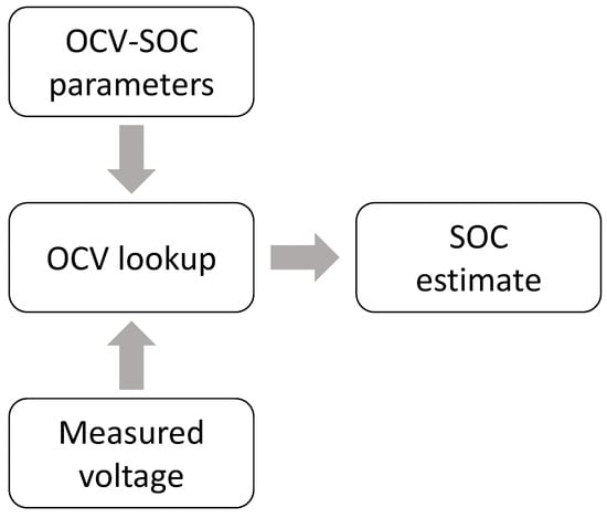
Figure 2. SOC estimation using OCV lookup.

1.1. Computing System Requirements

Figure 3 shows two different configurations of a battery management system, which consists of BFG only in this case, within a device. In the first case, shown in Figure 3a, the BFG lies within the operating system. In this case, the BFG algorithm, which is part of the operating system, enjoys a high-precision (i.e., high bit) computing environment. In the second case, shown in Figure 3b, the BFG lies outside the operating system. Many practical battery management systems fall under this category [29]. In this case, the BFG cannot afford the same high-precision computing environment available within an operating system.

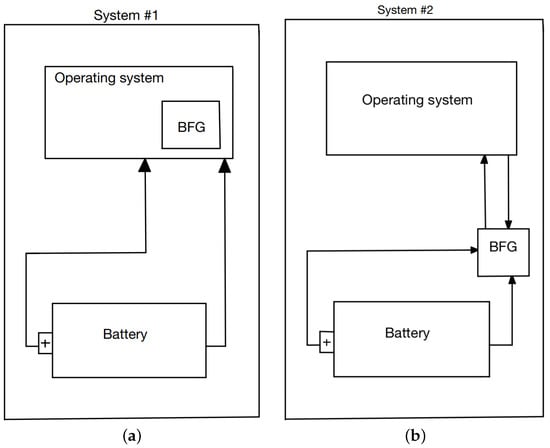
Figure 3. Types of BFG installation in a system. (a) BFG within OS. (b) BFG outside OS.

1.2. Rounding Errors

Table 1 lists various OCV-SOC models along with their model parameters reported in the literature. In order to perform SOC estimation, a BFG needs to store the OCV-SOC model parameters. The range of parameter values, indicated by the lowest and highest values in Table 1, is an indicator of system requirements. The range of OCV parameters needs to be compared with the range of SOC $\in [0,1]$ and the range of OCV ∈ [3 V, 4.2 V] that it represents. Similarly, the storage and processing of the OCV parameters is an important indicator of performance. The combined + 3 model needs a 30-bit system to store its parameters without any approximations—which is very significant for many low cost BFGs.

Table 1. Overview of existing models in the literature.

Reference	Model	Parameters	Lowest Parameter Value	Highest Parameter Value	System Requirement (Bits)
Combined [24]	$k_0+\frac{k_1}{s}+k_{2}s$ $+k_{3}ln\left(s\right)+k_{4}ln(1-s)$	$k_0=-1.041084,k_1=-0.809928,k_2=7.128030,k_3=-4.534755,$ $k_4=0.318780$	$k_3=-4.534755$	$k_2=7.128030$	25
Combined + 3 [17]	$k_0+\frac{k_1}{s}+\frac{k_2}{s^2}+\frac{k_3}{s^3}$ $+\frac{k_4}{s^4}+k_{5}s+k_{6}ln\left(s\right)$	$k_0=-9.081846,k_1=103.087009,k_2=-18.184590,k_3=2.062476,$ $k_4=-0.101779,k_5=-76.603691,k_6=141.199419,k_7=-1.116841$	$k_5=-76.603691$	$k_6=141.199419$	30
Polynomial [30]	$p_1+p_{2}s+p_3{s}^2$ $+p_4{s}^3+\frac{p_5}{s}+\frac{p_6}{s^2}$	$p_1=-3.882237,p_2=15.883339,p_3=-15.742669,p_4=6.780481,$ $p_5=1.737813,p_6=-0.153465$	$p_3=-15.742669$	$p_2=15.883339$	26
Sum of sine functions [31]	$a_1\sin (b_{1}s+c_1)$ $+a_2\sin (b_{2}s+c_2)$ $+a_3\sin (b_{3}s+c_3)$	$a_1=4.848,a_2=7.715,a_3=6.655,$ $b_1=1.512,b_2=4.756,b_3=4.928,$ $c_1=0.5841,c_2=1.99,c_3=5.038$	$a_2=7.715$	$c_1=0.5841$	16
Double exponential & quadratic [31,32,33]	$a_{1}exp\left(b_{1}s\right)$ $+a_{2}exp\left(b_{2}s\right)+c{s}^2$	$a_1=3.679,a_2=-0.2528,b_1=-0.1101,b_2=-6.829,c=0.9386$	$b_2=-6.829$	$a_1=3.679$	17
Fractional [34]	$k_0+k_{1}s+k_2{s}^2$ $-k_3{E}_{\alpha ,\beta }(-k_4{s}^{\alpha })$	$k_0=1.588,k_1=4.921,k_2=-3.073,k_3=-1.051,k_4=13.31,$ $\alpha =1.655,\beta =1.455$	$k_2=-3.073$	$k_4=13.31$	16
Polynomial & exponential [35]	$k_0+k_{1}s+k_2{s}^2$ $+k_3{s}^3+k_4{e}^{k_{5}s}$	$k_0=3.685,k_1=0.2156,k_2=-0.1178,k_3=0.3201,k_4=-1.031,$ $k_5=-35$	$k_5=-35$	$k_0=3.685$	16
Linear, logarithmic & exponential [36]	$a+b{(-lns)}^m+cs$ $+d{e}^{n(s-1)}$	$a=3.875,b=-0.3351,c=-0.5332,d=0.8315,$ $m=0.6537,n=0.6$	$c=-0.5332$	$a=3.875$	18
8th order polynomial [37,38]	$k_0+k_{1}s+k_2{s}^2$ $+k_3{s}^3+k_4{s}^4+k_5{s}^5$ $+k_6{s}^6+k_7{s}^7+k_8{s}^8$	$k_0=2.85,k_1=4.80,k_2=-17.8,k_3=38.59,k_4=4.91,k_5=-210.52,$ $k_6=433.98,k_7=-368.45,k_8=115.81$	$k_7=-368.45$	$k_6=433.98$	19
Weng’s model [39]	$k_0+k_1\frac{1}{1+e^{{\alpha }_1(s-{\beta }_1)}}$ $+k_2\frac{1}{1+e^{{\alpha }_2(s-{\beta }_2)}}$ $+k_3\frac{1}{1+e^{{\alpha }_3(s-1)}}$ $+k_4\frac{1}{1+e^{{\alpha }_{4}s}}+k_{5}s$	$k_0=3.4002,k_1=0.0080,k_2=0.0785,k_3=-0.2150,k_4=-1.3032,$ $k_5=0.0891,{\alpha }_1=-14,{\alpha }_2=-18,{\alpha }_3=28,{\alpha }_4=40$	${\alpha }_2=-18$	${\alpha }_4=40$	17
[40]	$k_0+k_1(1-e^{{\alpha }_{1}s})$ $+k_2(1-e^{\frac{{\alpha }_2}{1-s}})+k_{3}s$	Not available	-	-	-

In order to fit the parameters to the available space in low cost systems, it is a common practice to round them. Figure 4 shows the resulting OCV-SOC curve after rounding the parameters to lower significant numbers for some of the OCV-SOC models listed in Table 1. It is evident from Figure 4 that the OCV-SOC parametric representation of a battery may be significantly altered by rounding. This substantiates that approximating the parameters have serious effects on the resulting OCV-SOC curve for some models, whereas certain model parameters are robust to rounding. Table 1 and Figure 4 highlight the problems with existing OCV-SOC models in low-cost environments:

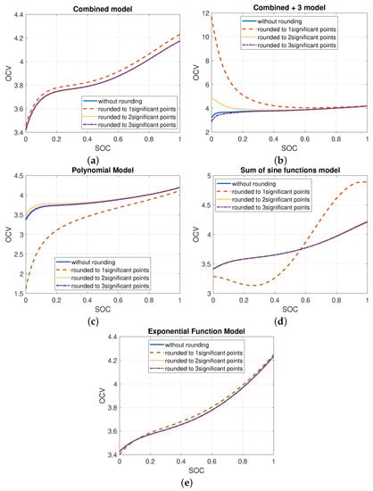
Figure 4. Rounding effects on accuracy in parametric models—(a) combined, (b) combined + 3, (c) polynomial, and (d) sum of sine functions (e) exponential.

(a)

Existing OCV-SOC models require high-bit computing resources for parameter storage and processing, and

(b)

Existing model predictions are susceptible to significant errors when the model parameters are rounded.

It is also noteworthy that existing OCV-SOC models listed in Table 1 rely on special functions, such as logarithmic and trigonometric functions. Most low-cost computing systems are unable to accurately compute these functions to the highest precision needed and approximations must be made. In [17], the errors involved in the numerical implementation of some of these functions are analyzed and alternate approaches are discussed for the implementation of OCV-SOC models in computationally restrictive environments.

1.3. Contribution of the Paper

The objective of this paper is to present OCV-SOC tables as an alternative to the model based OCV-SOC characterizations summarized in Table 1. Specifically, this paper presents the following contributions:

• For the first time, this paper relates the accuracy of SOC estimation to the numerical stability of the estimated OCV-SOC parameters due to a very common practice: rounding.
• The OCV-SOC table formulation is introduced as an objectively defined optimization problem.
• An approach is presented to formally quantify the performance of an OCV-SOC table: similarity metrics between a tabular OCV model and a hi-fidelity model is proposed as the performance metric of a particular tabular OCV model.
• Three new approaches are presented to create OCV-SOC tables based on hi-fidelity models.
• The resulting three tables are evaluated based on the metrics developed in this paper.

In order to make use of the proposed approach, the OCV-SOC parameters need to be first estimated offline using data collected in a high precision computing environment, such as a personal computer. After that, the proposed algorithms are employed to convert the OCV-SOC parameters into tabular OCV-SOC models. The tabular OCV-SOC models are created in a way that they can be stored and processed in much simpler computing environments, such as low-bit microcontrollers. It is also noteworthy that, in typical Li-ion batteries, the OCV ranges between 3 V and 4.2 V, whereas the SOC ranges between 0 and 1. The mentioned OCV-SOC range is true for all the models listed in Table 1. However, they are a much smaller range compared to the range of OCV-SOC parameters listed in Table 1. The proposed OCV-SOC table can be used for SOC estimation using state-space techniques, such as the extended Kalman filter [24] without requiring any additional parameters to be stored—since the change in SOC is much smaller between samples, linear interpolation is adequate to compute the required Jacobian for the EKF-based SOC estimation using the tabular OCV-SOC models.

The rest of the paper is organized as follows—Section 2 describes the problem of finding a non-uniform sampling of the OCV-SOC curve such that the sampling error is minimized. In Section 3, different approaches to developing a tabular OCV model are presented. Tabular approaches developed are implemented on the combined + 3 OCV model, which is discussed in Section 4. Results are presented in Section 6. Section 7 concludes the paper.

2. Problem Description

Consider a function $f\left(x\right)$ that is defined in $x\in [a,b]$. The goal is to represent this function at n discrete points, i.e.,

$$\begin{array}{c}\hfill g\left(x\right)=\sum _{i=1}^{n}f\left(x\right)\delta (x-x_i)i=1,\dots ,n\end{array}$$

(1)

such that the sampling error is minimized. Let us define the sampling error as the following

$$\begin{array}{c}\hfill e\left(x_i\right)=\frac{{\Delta }_i}{2}(f\left(x_i\right)+f\left(x_{i+1}\right))-{\int }_{x_i}^{x_{i+1}}f\left(x\right)dxi=2,\dots ,n\end{array}$$

(2)

where

$$\begin{array}{c}\hfill {\Delta }_i=x_{i+1}-x_i\end{array}$$

(3)

Figure 5 shows an example of sampling error when ${\Delta }_i=x_{i+1}-x_i=\Delta$, i.e., uniform sampling.

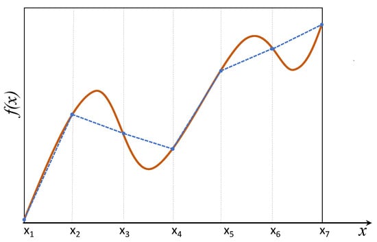
Figure 5. Uniform sampling: It can be seen that uniform sampling error (samples shown in dotted blue) increases with the magnitude of the curvature (function shown in red).

The objective of this paper is to find a non-uniform sampling of the function such that the sum of the squared sampling errors in (2) is minimized. That is, for a given n

$$\widehat{\mathcal{X}}=arg\underset{\mathcal{X}}{min}\sum _{i=1}^{n}e{\left(x_i\right)}^2$$

(4)

where $\mathcal{X}=\{x_1,x_2,\dots x_n\}$.

3. Solution Approaches

In this section, we describe several approaches to obtaining the samples.

3.1. Cumulative Approach

Let us define the area of $f\left(x\right)$ as

$$\begin{array}{c}\hfill {\mathcal{I}}_f={\int }_{x_1=a}^{x_n=b}f\left(x\right)dx\end{array}$$

(5)

Of the n points, $x_1=a$ and $x_n=b$ are preassigned. This leaves us with $L=n-2$ points to be assigned. The first unknown sample $x_2$ is selected such that

$$\begin{array}{c}\hfill {\int }_a^{x_2}f\left(x\right)dx=\frac{{\mathcal{I}}_f}{L+1}\end{array}$$

(6)

The subsequent samples $x_i,i=3,\dots ,n-1,$ are selected such that

$$\begin{array}{c}\hfill {\int }_{x_i-1}^{x_i}f\left(x\right)dx=\frac{{\mathcal{I}}_f}{L+1},i=3,\dots ,n-1\end{array}$$

(7)

Evidently, the last sample satisfies,

$$\begin{array}{c}\hfill {\int }_{x_{n-1}}^{x_b}f\left(x\right)dx=\frac{{\mathcal{I}}_f}{L+1}\end{array}$$

(8)

Figure 6 shows an example of cumulative tabular approach for $n=6$ points.

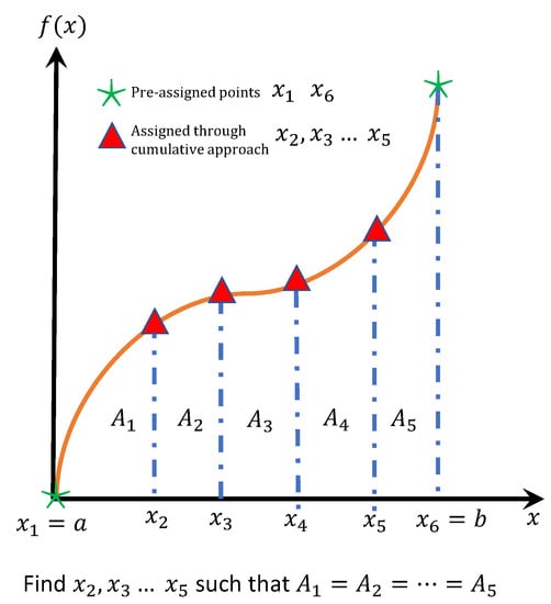
Figure 6. Pictorial representation of cumulative approach for $n=6$ points.

Algorithm 1 shows the procedural steps for placing table support points in the cumulative approach.

Algorithm 1 Cumulative approach.

1: Compute $I_f$ defined in (5) 2: Compute the first unknown sample according to (6) 3: Compute all samples until $n-1$ as defined in (7)

3.2. Inflection Point Approach

The curvature of a function is defined as

$$\begin{array}{c}\hfill C\left(x\right)=\frac{d^{2}f\left(x\right)}{d{x}^2}\end{array}$$

(9)

This approach assumes that the sign of the curvature changes at least once in the interval of $x\in [a,b]$. This is a valid assumption for all the OCV-SOC models. Let us assume, without loss of generality, that the sign of curvature changes at k (≥1) points and denote these k values as $x_{i_1},x_{i_2},\dots ,x_{i_k}$. That is, $x_i=\{x_{i_1},x_{i_2},\dots ,x_{i_k}\}$ will satisfy

$$\begin{array}{c}\hfill C\left(x_{i_j}\right)={\left.\frac{d^{2}f\left(x\right)}{d{x}^2}\right|}_{x=x_{i_j}}=0,j=1,2,\dots ,k\end{array}$$

(10)

These k values of $x_i$ are denoted as the “inflection points” or “critical points” from now on. The nature of the curve significantly changes at critical points, that is the function changes from convex to concave when the sign of the curvature changes from positive to negative, and vice versa; hence, one support point is assigned to each of the k critical points. Additionally, one support point is assigned, each at the start and end of the interval $[a,b]$, i.e., out of the n available support points, $k+2$ points—$x_1=a$, $x_n=b$ and the k values of $x_i$—are preassigned. These $k+2$ points are denoted as the “preassigned points” from now on. This leaves us with $n-k-2$ points to be assigned. In the remainder of this section, two different approaches are discussed to assign these remaining support points. Each of these two approaches consists of the following two steps:

(a)

Find number of support points to be allocated to each of the $k+1$ sections created by the k inflection points.

(b)

Placement of support points in each section.

The following notations will be used to describe these approaches:

$$\begin{array}{cc}\hfill r& =⌊\frac{n-k-2}{k+1}⌋\hfill \end{array}$$

(11)

$$\begin{array}{cc}\hfill m& =mod\left(\frac{n-k-2}{k+1}\right)\hfill \end{array}$$

(12)

where $\lfloor ·\rfloor$ denotes the floor operation and $mod\left(·\right)$ denotes the modulus operation. Here, one can see that

$$\begin{array}{c}\hfill n-k-2=r(k+1)+m\end{array}$$

(13)

The absolute area of the curvature in each of the $k+1$ sections is defined as

$$\begin{array}{c}\hfill A_j={\int }_{x_{i_j}}^{x_{i_{j+1}}}\left|C\left(x\right)\right|dxj=0,1,\dots ,k\end{array}$$

(14)

where $x_{i_0}=a$, $x_{i_{k+1}}=b,$ and $x_{i_1},x_{i_2},\dots ,x_{i_k}$ are defined according to (10). It is to be noted that $x_{i_0}=a$ and $x_{i_{k+1}}=b$ are not the critical points.

The next two subsections describe two different approaches to allocate these remaining $r(k+1)+m$ support points.

3.2.1. Approach-1 Based on Equal Distance in Each Section

In this approach, the goal is to place the $n-k-2$ support points equally between the k inflection points in each of the $k+1$ sections.

(a) Number of support points:

• Each section gets r support points.
• The remaining m support points are allocated as follows:
  If $m\le 3$, the m support points are assigned to section j such that

  $$\begin{array}{c}\hfill A_j>A_i\forall i=\{0,1,\dots ,k\},i\ne j\end{array}$$

  (15)
  Otherwise, if $m>3$ and m is even, $m/2$ support points are assigned to each of section $j_1$ and section $j_2$ such that

  $$\begin{array}{c}\hfill A_{j_1},A_{j_2}>A_i\forall i=\{0,1,\dots ,k\},i\ne j_1,i\ne j_2\end{array}$$

  (16)
  Otherwise, if $m>3$ and m is odd, $\lceil m/2\rceil$ support points are assigned to section $j_1$ such that

  $$\begin{array}{c}\hfill A_{j_1}>A_i\forall i=\{0,1,\dots ,k\},i\ne j_1\end{array}$$

  (17)
  $\lfloor m/2\rfloor$ support points are assigned to section $j_2$ such that

  $$\begin{array}{c}\hfill A_{j_2}>A_i\forall i=\{0,1,\dots ,k\},i\ne j_1,i\ne j_2\end{array}$$

  (18)

(b) Placement of support points: Once the number of points in each section is allocated, the points in each section are then placed equally distant within that section. Let us assume that section j, which is bounded by $x_{i_j}$ and $x_{i_{j+1}}$, was assigned L support points. The location of these L support points can be written as

$$\begin{array}{c}\hfill x_l=x_{i_j}+d\ast l,l=1,2,\dots ,L\end{array}$$

(19)

where

$$\begin{array}{c}\hfill d=\frac{x_{i_{j+1}}-x_{i_j}}{L+1}\end{array}$$

(20)

where the distance in each section is determined by the difference between the preassigned points of that section divided by the total number of points plus one of that section.

Figure 7 explains allocation and placement of tabular support points by the inflection-1 approach for the example of a single inflection point of $f\left(x\right)$.

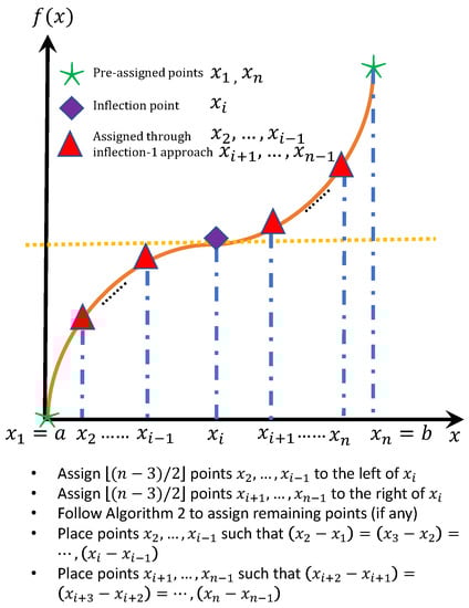
Figure 7. Pictorial representation of inflection-1 approach considering one inflection point.

Algorithm 2 shows the procedural steps for allocating and placing table support points in the inflection-1 approach.

3.2.2. Approach-2 Based on Equal Area in Each Section

In this approach, the goal is to place the $n-k-2$ support points as a ratio of the area under the curvature defined in (14).

(a) Number of support points:

• Each section j gets $r_j$ support points as follows

  $$\begin{array}{c}\hfill r_j=⌊\frac{A_j}{{\sum }_{i=0}^k{A}_i}⌋\times (n-k-2)\end{array}$$

  (21)

  where $j=0,\dots ,k$ and the remaining number of points m is given by

  $$\begin{array}{c}\hfill m=n-k-2-\sum _{j=0}^k{r}_j\end{array}$$

  (22)
• The remaining m support points are allocated as follows: The section with the highest area under the curvature gets one point; next, the section with the second highest area under the curvature gets one point; this is continued until all the remaining m points are assigned to a section.

(b) Placement of support points: Once the number of points in each section is allocated, the points in each section are then placed based on equal area sampling in each of those sections. The approach to assign support points for each section is very similar to the approach described in Section 3 with one difference: In Section 3, area under $f\left(x\right)$ is considered; here, the area under the curvature $C\left(x\right)$ is considered.

Algorithm 2 Inflection-1 approach.

(I) Allocation of support points 1: Compute $C\left(x_{i_j}\right)$, i.e., determine k inflection points of (10) 2: Compute r defined in (11) 3: Allocate r points to each of the $k+1$ sections created by the k inflection points 4: Compute the remaining points, m, defined in (12) 5: if $m\le 3$ then 6:     assign all m points to section $j\mathrm{s}.\mathrm{t}.A_j>A_i\forall i=\{0,1,\dots ,k\},i\ne j$ ; where $A_j$ is defined in (14) 7: else 8:     if m is even then 9:         assign $m/2$ points each to sections $j_1,j_2\mathrm{s}.\mathrm{t}.A_{j_1},A_{j_2}>A_i\forall i=\{0,1,\dots ,k\},$$i\ne j_1,i\ne j_2$ 10:     else 11:         (a) assign $\lceil m/2\rceil$ points to section $j_1\mathrm{s}.\mathrm{t}.A_{j_1}>A_i\forall i=\{0,1,\dots ,k\},i\ne j_1$ 12:         (b) assign $\lfloor m/2\rfloor$ points to section $j_2\mathrm{s}.\mathrm{t}.A_{j_2}>A_i\forall i=\{0,1,\dots ,k\},i\ne j_1,$$i\ne j_2$ 13:     end if 14: end if (II) Placement of support points 15: For each section, place support points according to the distance d defined for that section in (20).

Figure 8 explains the allocation and placement of tabular support points by the inflection-2 approach for the example of a single inflection point of $f\left(x\right)$.

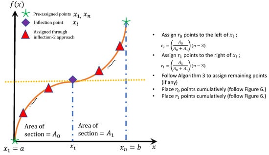
Figure 8. Pictorial representation of inflection-2 approach considering one inflection point.

Algorithm 3 shows the procedural steps for allocating and placing table support points in the inflection-2 approach.

Algorithm 3 Inflection-2 approach.

(I) Allocation of support points 1: Compute $C\left(x_{i_j}\right)$, i.e., determine k inflection points of (10) 2: Compute $r_j$ defined in (21) 3: Allocate $r_j$ points to each jth section, where $j=0,\dots ,k$ 4: Compute the remaining points, m, defined in (22) 5: Place each point in m to section j from the largest to the least area. (II) Placement of support points 6: For each section, place support points based on the cumulative approach in Algorithm 1

In Section 4, the approaches presented in this section are elaborated using a particular OCV-SOC curve.

4. Implementation on OCV Model

In this section, the combined + 3 model from Table 1 is taken as the reference OCV-SOC model to implement the tabular approaches presented in Section 3. The combined + 3 OCV-SOC model is given by,

$$\begin{array}{cc}\hfill V_{\circ }\left(s\right)=& k_0+\frac{k_1}{s}+\frac{k_2}{s^2}+\frac{k_3}{s^3}+\frac{k_4}{s^4}\hfill \\ \hfill & +k_{5}s+k_{6}ln\left(s\right)+k_{7}ln(1-s)\hfill \end{array}$$

(23)

where it is assumed that the OCV parameters $k_0,k_1,\dots k_7$ are obtained by linearly scaling $s\in [0,1]$ to lie between $[ϵ,1-ϵ]$ [41]. The implementation detailed below assumes the parameters of the combined + 3 model as those provided in Table 1 with $ϵ=0.175$.

4.1. Cumulative Approach

The area under the OCV-SOC curve, shown in Figure 9a, is given by

$$\begin{array}{cc}\hfill {\mathcal{I}}_f& ={\int }_{ϵ}^{1-ϵ}{V}_{\circ }\left(s\right)ds\hfill \\ \hfill & =[k_{0}s+k_{1}ln\left(s\right)-\frac{k_2}{s}-\frac{k_3}{2s^2}-\frac{k_4}{3s^3}+k_5\frac{s^2}{2}\hfill \\ \hfill & +k_6(sln\left(s\right)-s)-k_7((1-s)ln(1-s)-(1-s)){]}_{ϵ}^{1-ϵ}\hfill \end{array}$$

(24)

$$\begin{array}{c}=2.5073\hfill \end{array}$$

(25)

Out of the n available support points, $x_1=ϵ$ and $x_n=1-ϵ$ are preassigned. The remaining $L=n-2$ points are found as follows. The first unknown support point $x_2$ can be found such that

$$\begin{array}{cc}\hfill & {\int }_{x_1=ϵ}^{x_2}{V}_{\circ }\left(s\right)ds=[k_{0}s+k_{1}ln\left(s\right)-\frac{k_2}{s}-\frac{k_3}{2s^2}-\frac{k_4}{3s^3}+k_5\frac{s^2}{2}\hfill \\ \hfill & +k_6(sln\left(s\right)-s)-k_7((1-s)ln(1-s)-(1-s)){]}_{ϵ}^{x_2}=\frac{2.5073}{L+1}\hfill \end{array}$$

(26)

Similarly, the second unknown point $x_3$ can be found such that

$$\begin{array}{c}\hfill {\int }_{x_2}^{x_3}{V}_{\circ }\left(s\right)ds=\frac{2.5073}{L+1}\end{array}$$

(27)

By continuing in a similar fashion, the $(n-1)\mathrm{th}$ point can be found as

$$\begin{array}{c}\hfill {\int }_{x_{n-2}}^{x_{n-1}}{V}_{\circ }\left(s\right)ds=\frac{2.5073}{L+1}\end{array}$$

(28)

The nth point, $x_n=1-ϵ$, automatically satisfies

$$\begin{array}{c}\hfill {\int }_{x_{n-1}}^{1-ϵ}{V}_{\circ }\left(s\right)ds=\frac{2.5073}{L+1}\end{array}$$

(29)

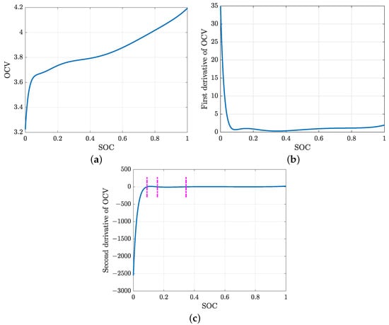
Figure 9. OCV model and its first two derivatives—(a) OCV model-$V_{\circ }\left(s\right)$, (b) first derivative-$V_{\circ }^{\prime }\left(s\right)$, and (c) second derivative-$V_{\circ }^{″}\left(s\right)$.

A demonstration of this approach for different numbers of support points n is presented in Section 6.

4.2. Inflection Point Approach

In this approach, we have to find the points where the curvature of the OCV model, $C\left(s\right)=\frac{d^2{V}_{\circ }\left(s\right)}{d{s}^2}$ = 0 and find locations where it changes sign.

$$\begin{array}{cc}\hfill \frac{d^2{V}_{\circ }\left(s\right)}{d{s}^2}=& 2\frac{k_1}{s^3}+6\frac{k_2}{s^4}+12\frac{k_3}{s^5}+20\frac{k_4}{s^6}-\frac{k_6}{s^2}-\frac{k_7}{{(1-s)}^2}=0\hfill \end{array}$$

(30)

There are six roots of the equation above, however only three are in the range, $s\in [ϵ,1-ϵ]$. Figure 9 represents the curvature of the OCV model considered and the inflection points are marked. The inflection points are thus, $s=[0.2334,0.2773,0.3995]$ in the range $[ϵ,1-ϵ]$ . These three inflection points create four sections in the OCV-SOC curve. The inflection points, along with the points at $s=ϵ$ and $s=1-ϵ$, form the $k+2=5$ preassigned points, $[ϵ,0.2334,0.2773,0.3995,1-ϵ]$. With the identified inflection points, approaches as discussed in the previous section help in determining the support points for the tabular OCV model.

4.2.1. Approach-1 Based on Equal Distance

• The first step is to allocate the number of points to each of the four sections, given the total number of support points, n. Denote the number of points allocated to each section by an array, say

  $$\begin{array}{c}\hfill L=[L_0,L_1,L_2,L_3]\end{array}$$

  (31)

  where each $L_j,j=0,1,2,3$ is determined by the logic discussed in Section 3.2.1.
• The distance between the points in each section is then the difference between the preassigned points of that section divided by the number of points plus one of the corresponding section, which is

  $$\begin{array}{cc}\hfill [d_0,d_1,d_2,d_3]=& \left[\frac{0.2334-ϵ}{L_0+1},\frac{0.2773-0.2334}{L_1+1},\right.\hfill \\ \hfill & \left.\frac{0.3995-0.2773}{L_2+1},\frac{(1-ϵ)-0.3995}{L_3+1}\right]\hfill \end{array}$$

  (32)
• Points in the first section are then placed at,

  $$\begin{array}{c}\hfill x_l=ϵ+d_{0}l\end{array}$$

  (33)

  where $l=1,\dots ,L_0$, while in the second section, points are placed at,

  $$\begin{array}{c}\hfill x_l=0.2334+d_{1}l\end{array}$$

  (34)

  where $l=1,\dots ,L_1$.
• Similarly, points in the third and fourth section are placed accordingly.
• Thus, $x(1:n)$ and the corresponding OCV at those points form the support (SOC, OCV) pairs of the tabular OCV model.

4.2.2. Approach-2 Based on Equal Area

• The first step is to allocate the number of points to each of the four sections, given the total number of support points, n. Denote the number of points allocated to each section as in (31).
• The absolute area of each of the sections is determined as in (14). Denote the absolute area of each of the sections as $[A_0,A_1,A_2,A_3]$.
• The points in the first section can thus be determined as

  $$\begin{array}{c}\hfill {\int }_{x_i}^{x_{i+1}}C\left(x\right)dx=\frac{A_0}{L_0+1},i=1,\dots ,L_0\end{array}$$

  (35)

  while in the second section, points are determined as

  $$\begin{array}{c}\hfill {\int }_{x_i}^{x_{i+1}}C\left(x\right)dx=\frac{A_1}{L_1+1},i=1,\dots ,L_1\end{array}$$

  (36)
• Similarly, points in the third and fourth section are placed accordingly.
• Thus, $x(1:n)$ and the corresponding OCV at those points form the support (SOC, OCV) pairs of the tabular OCV model.

5. Experimental Details

The proposed approach is demonstrated using data collected from four commercially available Li-ion batteries.

5.1. Batteries Tested

The model number of the battery is Samsung-30T INR21700. One of the four identical cells is shown in Figure 10 and the features of the cell is summarized in Table 2. The four tested battery cells are labeled ‘C1202’, ‘C1203’, ‘C1204’, and ‘C1205’ and will be referred using these labels in the remainder of this paper.

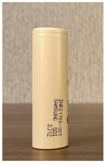
Figure 10. Samsung-30T INR21700 Li-ion battery.

Table 2. Specifications of Li-ion battery.

Specification	Value (Unit)
Nominal capacity	3000 mAh
Max. continuous discharge current	35 A
Nominal voltage	3.6 V
Height	70 mm
Diameter	21 mm
Weight	70 g
Internal resistance	15 m $\mathsf{\Omega }$

5.2. Testing Equipment

The data from batteries is collected using Arbin battery cycler (LBT21084, Arbin Instruments, College Station, TX, USA). It has 16 independently controlled channels, each with a voltage range of 0–5 V and a current range of ±10 A. Four channels were used to collect OCV-SOC data simultaneously from four cells at room temperature. The experimental setup used for testing the batteries is shown in Figure 11.

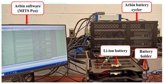
Figure 11. Experimental setup for battery testing.

5.3. OCV-SOC Characterization Test

A constant current–constant voltage (CC-CV) charging regime is followed to fully charge the battery before conducting an OCV-SOC test. A low current slow discharge–charge of the battery is pursued to perform the OCV-SOC test.

• A constant current is supplied to the battery until the terminal voltage reaches 4.2 V.
• The terminal voltage is maintained at 4.2 V for constant voltage charging until the current drops to 0.01 A.
• The battery is rested for one hour.
• A constant current of $C/30$ is supplied to slowly discharge the battery for thirty hours until the SOC reaches 0%. A rest of 1 h follows, before the battery is charged back again by $C/30$ for thirty hours until the SOC reaches 100%.

The battery terminal voltage and current data recorded by Arbin cycler during the OCV experiment is shown in Figure 12. The data is then processed to obtain the typical OCV-SOC curve represented by the combined + 3 model in (23).

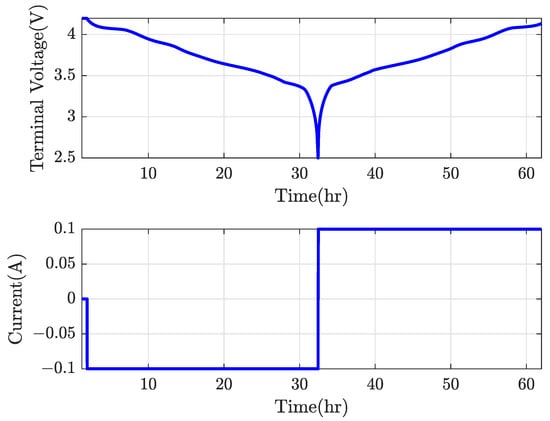
Figure 12. V-I data in OCV test.

5.4. OCV Parameter Estimation

The terminal voltage, $V_t$ and current, I, recorded from the battery during OCV experiment can be written in the form of observation model as follows:

$$V_t=V_o\left(s\right)+IR+n$$

(37)

where $V_o\left(s\right)$ is the OCV of the battery represented using the combined + 3 model in (23) as a function of the SOC, s, and R denotes the internal resistance of the battery. n is the zero-mean Gaussian noise in the measurement of voltage.

The estimation of OCV parameters is the solution to the least-squares problem formulated using the observation model in (37) as follows:

$$\begin{array}{cc}\hfill V_t& =[1\frac{1}{s}\frac{1}{s^2}\frac{1}{s^3}\frac{1}{s^4}sln\left(s\right)ln(1-s)]\left[\begin{array}{c}{\mathbf{k}}_{\circ }\\ R\end{array}\right]+n\hfill \\ \hfill & =\mathbf{p}{\left(s\right)}^T\mathbf{k}+n\hfill \end{array}$$

(38)

where

$$\begin{array}{cc}\hfill \mathbf{p}{\left(s\right)}^T& =[1\frac{1}{s}\frac{1}{s^2}\frac{1}{s^3}\frac{1}{s^4}sln\left(s\right)ln(1-s)]\hfill \\ \hfill \mathbf{k}& =\left[\begin{array}{c}{\mathbf{k}}_{\circ }\\ R\end{array}\right]\hfill \\ \hfill {\mathbf{k}}_{\circ }& ={\left[{\kappa }_0{\kappa }_1{\kappa }_2{\kappa }_3{\kappa }_4{\kappa }_5{\kappa }_6{\kappa }_7\right]}^T\hfill \end{array}$$

A batch of L observations of (38) from the characterization test, spanning the entire range of OCV and SOC, can be written in the vector observation form as

$$\begin{array}{cc}\hfill {\mathbf{v}}_t& ={\mathbf{p}}^{\mathbf{T}}\mathbf{k}+\mathbf{n}\hfill \end{array}$$

(39)

where the data (of length L) is collected during the entire SOC region as required in OCV-SOC characterization [17]. For example, the data collected from each battery is similar to the one shown in Figure 12.

The OCV parameters can then be estimated through the least squares approach as follows [17]:

$$\begin{array}{c}\hfill \widehat{\mathbf{k}}=arg\underset{\mathbf{k}}{min}\parallel {\mathbf{v}}_t-{\mathbf{p}}^{\mathbf{T}}\mathbf{k}\parallel \end{array}$$

(40)

Table 3 gives the values of the obtained OCV parameters for all four battery cells obtained by incorporating a linear scaling approach presented in [41].

Table 3. Obtained OCV-SOC parameters.

	C1202	C1203	C1204	C1205
$k_0$	−7.583571	−7.97819289	−8.066393564	−8.958403863
$k_1$	167.937349	163.9771372	162.9340579	142.8466347
$k_2$	−28.707024	−28.0994585	−27.93066927	−24.66098891
$k_3$	3.179598	3.119518894	3.101048887	2.753908717
$k_4$	−0.154205	−0.151625024	−0.150700733	−0.13454535
$k_5$	−136.082267	−132.0073615	−130.9737274	−111.5824628
$k_6$	239.483802	233.2027873	231.5789098	201.0624577
$k_7$	−1.939093	−1.842637102	−1.825728052	−1.337800859

Once the OCV parameters, ${\mathbf{k}}_{\circ }$, are determined, OCV-SOC tables can be created using one of the three approaches detailed in Section 3.

6. Results

In this section, results for the proposed tabular OCV modeling approaches, described in Section 3, are illustrated using data collected from C1202.

Figure 13a shows the plot of the OCV-SOC curve, corresponding to the combined + 3 model (23). The first and second derivatives of the curve is shown in Figure 13b and Figure 13c, respectively.

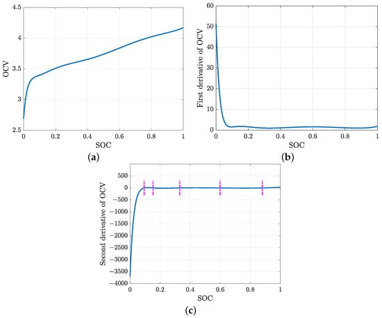
Figure 13. OCV model and its first two derivatives—(a) OCV model-$V_{\circ }\left(s\right)$, (b) first derivative-$V_{\circ }^{\prime }\left(s\right)$, and (c) second derivative- $V_{\circ }^{″}\left(s\right)$.

Figure 14 shows a comparison of the three approaches. The solid red line shows the parameterized OCV-SOC curve (the same curve as in Figure 13a) and the blue‘*’ markers denote the tabular entries obtained using the proposed approaches. The left column of Figure 14 summarizes the results for $n=16$ support points and the right column summarizes the results for $n=32$ support points. The first, second, and third rows of Figure 14 show the true OCV-SOC curve and the resulting tabular approximations using the cumulative, inflection-1, and inflection-2 approaches. The last row of Figure 14 shows the SOC lookup error based on the resulting tabular OCV model for each approach. Here, the SOC lookup error is computed for each possible OCV within the given range by employing linear interpolation to find SOC for a given OCV. Both the cumulative and the inflection-1 approaches produce less than 1% in SOC lookup error with just 32 points.

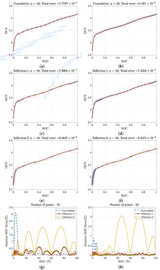
Figure 14. Tabular approximation error—(a) cumulative-16 point, (b) cumulative-32 point, (c) inflection-1-16 point, (d) inflection-1-32 point, (e) inflection-2-16 point, (f) inflection-2-32 point, (g) SOC lookup error for 16 points, and (h) SOC lookup error for 32 points.

Table 4 shows the obtained tabular OCV model for the inflection-1 approach for $n=16$ points, for all four batteries. It can be noticed that the variance in the values is less compared to the model parameters shown in Table 3.

Table 4. Tabular OCV model.

C1202		C1203		C1204		C1205
SOC	OCV	SOC	OCV	SOC	OCV	SOC	OCV
0	2.6929	0	2.6902	0	2.7003	0	2.7296
0.0236	3.1683	0.0238	3.1678	0.0236	3.1692	0.0246	3.1836
0.0473	3.3177	0.0476	3.3175	0.0472	3.3171	0.0492	3.3247
0.0709	3.3668	0.0714	3.3667	0.0708	3.3658	0.0738	3.3725
0.0945	3.3923	0.0951	3.3923	0.0944	3.3910	0.0984	3.3991
0.1238	3.4225	0.1245	3.4226	0.1242	3.4216	0.1254	3.4270
0.1530	3.4561	0.1539	3.4562	0.1539	3.4557	0.1523	3.4570
0.2417	3.5478	0.2428	3.5481	0.2432	3.5479	0.2416	3.5469
0.3303	3.6094	0.3318	3.6103	0.3325	3.6101	0.3308	3.6099
0.4644	3.7059	0.4660	3.7075	0.4673	3.7073	0.4706	3.7129
0.5985	3.8368	0.6003	3.8384	0.6021	3.8384	0.6103	3.8511
0.7391	3.9740	0.7418	3.9760	0.7425	3.9748	0.7618	3.9999
0.8798	4.0759	0.8833	4.0784	0.8829	4.0773	0.9132	4.1080
0.9199	4.1018	0.9222	4.1036	0.9219	4.1029	0.9421	4.1260
0.9599	4.1315	0.9611	4.1321	0.9610	4.1319	0.9711	4.1453
1.0000	4.1710	1.0000	4.1693	1.0000	4.1696	1.0000	4.1676

Figure 15 shows the tabular approximation error defined in (2) for all the three approaches for different number of support points, n. Here, it can be seen that each approach results in reduced error with increasing number of points. The inflection-1 approach consistently outperforms the other two approaches.

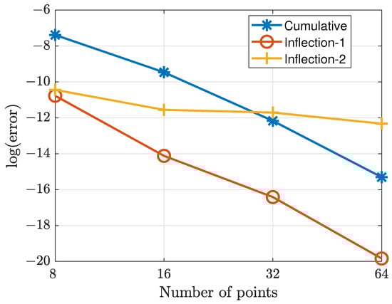
Figure 15. Tabular approximation error vs. number of points.

Figure 16 shows the results of rounding the digits of tabular approaches. This figure must be viewed in comparison to Figure 4, which shows how rounding in parametric models resulted in significantly altered OCV-SOC curves.

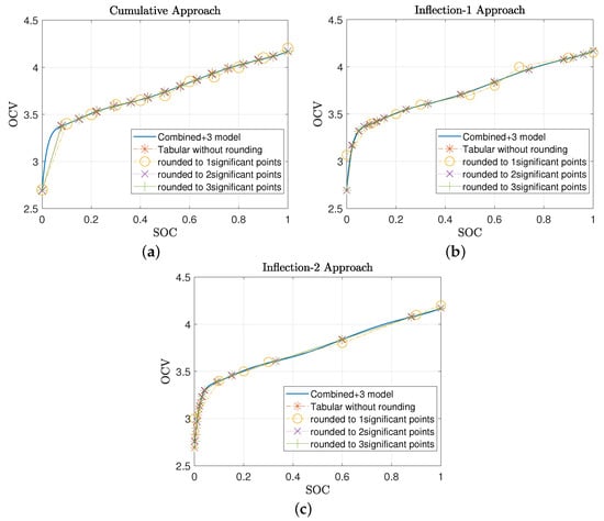
Figure 16. Effect of rounding in tabular models—(a) cumulative, (b) inflection-1,and (c) Inflection-2.

The following two metrics are used to quantify the distortion of an OCV curve in relation to the original, high-precision model in (23).

$$\begin{array}{cc}\hfill \mathrm{KL}\mathrm{divergence}& =\sum _{i=1}^n{\mathrm{OCV}}_0\left(s_i\right)log\left(\frac{{\mathrm{OCV}}_0\left(s_i\right)}{{\mathrm{OCV}}_1\left(s_i\right)}\right)\hfill \end{array}$$

(41)

$$\begin{array}{cc}\hfill \mathrm{Cos}\mathrm{ine}\mathrm{distance}& =1-\frac{{\sum }_{i=1}^n{\mathrm{OCV}}_0\left(s_i\right){\mathrm{OCV}}_1\left(s_i\right)}{\sqrt{{\sum }_{i=1}^n{\mathrm{OCV}}_0^2\left(s_i\right)}\sqrt{{\sum }_{j=1}^n{\mathrm{OCV}}_1^2\left(s_i\right)}}\hfill \end{array}$$

(42)

where $s_1,s_2,\dots ,s_n$ span the entire SOC range [0, 1]. Using the above two metrics, the combined + 3 parametric and the inflection-1 tabular models with rounding are compared to the true combined + 3 model without any rounding. The results of such a comparison are tabulated in Table 5.

Table 5. KL divergence and cosine distance.

	Parametric Combined + 3 Model			Tabular Inflection-1 Model
	Rounded to 1 Digit	Rounded to 2 Digits	Rounded to 3 Digits	Without Rounding	Rounded to 1 Digit	Rounded to 2 Digits	Rounded to 3 Digits
KL divergence	0.044608	0.002606	0.000167	2.41 × 10${}^{-8}$	4.13 × 10${}^{-5}$	2.54 × 10${}^{-7}$	2.76 × 10${}^{-8}$
Cosine distance	0.058112	0.00275	0.000147	2.49 × 10${}^{-8}$	3.77 × 10${}^{-5}$	2.54 × 10${}^{-7}$	2.85 × 10${}^{-8}$

A uniform SOC grid of hundred samples is selected. The OCV values corresponding to the SOC grid for the parametric combined + 3 model are obtained through (23) by rounding the OCV parameters, $k_0,k_1,\dots k_7$, from one to three significant digits. For the tabular model, since, the inflection-1 method performs significantly better than the other two tabular models, the OCV values corresponding to the SOC grid are found by linear interpolation using Table 4 inflection-1 values as is and by rounding the table values from one to three significant digits. The OCV values obtained from rounding the parameters of the OCV model and from rounding the table are compared to the OCV values of the true combined + 3 model without any rounding in (23) through KL divergence and cosine distance and the following observations are made.

It can be seen that, the KL divergence for the parametric model with rounding is greater than that for the tabular model with rounding. Hence, the parametric model with rounding is more divergent from the true model as compared to the tabular model with rounding. This clearly indicates that, even with rounding, the tabular approach performs better than the parametric approach. Cosine distance, another indicator of divergence, similar to KL, also shows how rounding in the parametric model largely affects its approximation to the true combined + 3 model, as compared to the tabular model with rounding. Within the parametric and tabular models themselves, rounding the significant digits from three to one renders the approximation to be more divergent from the true model. Thus, the rounding effects seen visually in the parametric and tabular models in Figure 4 and Figure 16, respectively, are also formally validated through the KL divergence and cosine distance metrics in Table 5. This clearly concludes how even with rounding, the tabular approach outperforms the parametric model.

7. Conclusions

This papers outlines the difficulties in traditional OCV-SOC characterization employed in battery management systems. It is shown that traditional approaches, which store the OCV-SOC characteristics in the form of parameterized functions, suffer from high computing requirements and susceptibility to rounding errors. As opposed to storing the parameters of the OCV-SOC functions, the advantages of a tabular OCV-SOC model are detailed in this paper.

Three different approaches are presented to convert traditional, high-precision OCV-SOC parameters into OCV-SOC tables. The proposed approaches can be employed to create OCV-SOC tables based on the available computing capabilities. It is also possible to select tabular OCV-SOC models that guarantee a certain maximum SOC estimation error. Memory and computational power are valuable resources of a BMS in battery packs. It is shown that significant savings in memory can be achieved by the proposed tabular OCV-SOC models. The resulting OCV-SOC table is shown to be less sensitive to rounding, compared to their parametric counterparts.

The present work can be extended in several of the following directions (i) the proposed algorithms should be implemented in a BMS for SOC estimation; (ii) currently, the proposed tabular approaches are developed on a fitted OCV-SOC combined + 3 model; future work should be focused on developing these approaches directly from battery experimental data; (iii) applicability of the proposed approach in different battery chemistries, for example LFP batteries, needs to be investigated; and (iv) performance of the proposed tabular approaches in the implementation of Kalman Filter needs to be analyzed.

References

- Hasan, M.K.; Mahmud, M.; Ahasan Habib, A.; Motakabber, S.; Islam, S. Review of electric vehicle energy storage and management system: Standards, issues, and challenges. J. Energy Storage 2021, 41, 102940. [Google Scholar] [CrossRef]
- Balasingam, B.; Ahmed, M.; Pattipati, K. Battery management systems—Challenges and some solutions. Energies 2020, 13, 2825. [Google Scholar] [CrossRef]
- Hannan, M.A.; Hoque, M.M.; Hussain, A.; Yusof, Y.; Ker, P.J. State-of-the-art and energy management system of lithium-ion batteries in electric vehicle applications: Issues and recommendations. IEEE Access 2018, 6, 19362–19378. [Google Scholar] [CrossRef]
- Wang, X.; Wei, X.; Zhu, J.; Dai, H.; Zheng, Y.; Xu, X.; Chen, Q. A review of modeling, acquisition, and application of lithium-ion battery impedance for onboard battery management. eTransportation 2021, 7, 100093. [Google Scholar] [CrossRef]
- Balasingam, B.; Pattipati, K.R. On the identification of electrical equivalent circuit models based on noisy measurements. IEEE Trans. Instrum. Meas. 2021, 70, 1–16. [Google Scholar] [CrossRef]
- Zhou, Z.; Cui, Y.; Kong, X.; Li, J.; Zheng, Y. A fast capacity estimation method based on open circuit voltage estimation for linixcoymn1-xy battery assessing in electric vehicles. J. Energy Storage 2020, 32, 101830. [Google Scholar] [CrossRef]
- Pan, W.; Luo, X.; Zhu, M.; Ye, J.; Gong, L.; Qu, H. A health indicator extraction and optimization for capacity estimation of li-ion battery using incremental capacity curves. J. Energy Storage 2021, 42, 103072. [Google Scholar] [CrossRef]
- Zheng, Y.; Cui, Y.; Han, X.; Dai, H.; Ouyang, M. Lithium-ion battery capacity estimation based on open circuit voltage identification using the iteratively reweighted least squares at different aging levels. J. Energy Storage 2021, 44, 103487. [Google Scholar] [CrossRef]
- Movahedi, H.; Tian, N.; Fang, H.; Rajamani, R. Hysteresis compensation and nonlinear observer design for state-of-charge estimation using a nonlinear double-capacitor li-ion battery model. IEEE/ASME Trans. Mechatron. 2021, 27, 594–604. [Google Scholar] [CrossRef]
- Ni, Z.; Yang, Y. A combined data-model method for state-of-charge estimation of lithium-ion batteries. IEEE Trans. Instrum. Meas. 2021, 71, 1–11. [Google Scholar] [CrossRef]
- Deng, Z.; Hu, X.; Lin, X.; Xu, L.; Che, Y.; Hu, L. General discharge voltage information enabled health evaluation for lithium-ion batteries. IEEE/ASME Trans. Mechatron. 2020, 26, 1295–1306. [Google Scholar] [CrossRef]
- Bian, X.; Liu, L.; Yan, J.; Zou, Z.; Zhao, R. An open circuit voltage-based model for state-of-health estimation of lithium-ion batteries: Model development and validation. J. Power Sources 2020, 448, 227401. [Google Scholar] [CrossRef]
- Hasib, S.A.; Islam, S.; Chakrabortty, R.K.; Ryan, M.J.; Saha, D.K.; Ahamed, M.H.; Moyeen, S.I.; Das, S.K.; Ali, M.F.; Islam, M.R.; et al. A comprehensive review of available battery datasets, rul prediction approaches, and advanced battery management. IEEE Access 2021, 9, 86166–86193. [Google Scholar] [CrossRef]
- Zhou, W.; Zheng, Y.; Pan, Z.; Lu, Q. Review on the battery model and soc estimation method. Processes 2021, 9, 1685. [Google Scholar] [CrossRef]
- How, D.N.T.; Hannan, M.A.; Lipu, M.S.H.; Ker, P.J. State of charge estimation for lithium-ion batteries using model-based and data-driven methods: A review. IEEE Access 2019, 7, 136116–136136. [Google Scholar] [CrossRef]
- Movassagh, K.; Raihan, A.; Balasingam, B.; Pattipati, K. A critical look at coulomb counting approach for state of charge estimation in batteries. Energies 2021, 14, 4074. [Google Scholar] [CrossRef]
- Pattipati, B.; Balasingam, B.; Avvari, G.; Pattipati, K.; Bar-Shalom, Y. Open circuit voltage characterization of lithium-ion batteries. J. Power Sources 2014, 269, 317–333. [Google Scholar] [CrossRef]
- Tong, S.; Klein, M.P.; Park, J.W. On-line optimization of battery open circuit voltage for improved state-of-charge and state-of-health estimation. J. Power Sources 2015, 293, 416–428. [Google Scholar] [CrossRef]
- Dang, X.; Yan, L.; Xu, K.; Wu, X.; Jiang, H.; Sun, H. Open-circuit voltage-based state of charge estimation of lithium-ion battery using dual neural network fusion battery model. Electrochim. Acta 2016, 188, 356–366. [Google Scholar] [CrossRef]
- Li, L.-L.; Liu, Z.-F.; Wang, C.-H. The open-circuit voltage characteristic and state of charge estimation for lithium-ion batteries based on an improved estimation algorithm. J. Test. Eval. 2018, 48, 1712–1730. [Google Scholar] [CrossRef]
- Susanna, S.; Dewangga, B.R.; Wahyungoro, O.; Cahyadi, A.I. Comparison of simple battery model and thevenin battery model for soc estimation based on ocv method. In Proceedings of the 2019 International Conference on Information and Communications Technology, Yogyakarta, Indonesia, 24–25 July 2019; pp. 738–743. [Google Scholar]
- Wang, Q.; Qi, W. New soc estimation method under multi-temperature conditions based on parametric-estimation ocv. J. Power Electron. 2020, 20, 614–623. [Google Scholar] [CrossRef]
- Jibhkate, U.N.; Mujumdar, U.B. Development of low complexity open circuit voltage model for state of charge estimation with novel curve modification technique. Electrochim. Acta 2022, 429, 140944. [Google Scholar] [CrossRef]
- Plett, G.L. Extended kalman filtering for battery management systems of lipb-based hev battery packs: Part 2. modeling and identification. J. Power Sources 2004, 134, 262–276. [Google Scholar] [CrossRef]
- Fathoni, G.; Widayat, S.A.; Topan, P.A.; Jalil, A.; Cahyadi, A.I.; Wahyunggoro, O. Comparison of state-of-charge (soc) estimation performance based on three popular methods: Coulomb counting, open circuit voltage, and kalman filter. In Proceedings of the 2017 2nd International Conference on Automation, Cognitive Science, Optics, Micro Electro-Mechanical System, and Information Technology, Jakarta, Indonesia, 23–24 October 2017; pp. 70–74. [Google Scholar]
- Xu, X.; Wu, D.; Yang, L.; Zhang, H.; Liu, G. State estimation of lithium batteries for energy storage based on dual extended kalman filter. Math. Probl. Eng. 2020, 2020, 6096834. [Google Scholar] [CrossRef]
- Gismero, A.; Schaltz, E.; Stroe, D.-I. Recursive state of charge and state of health estimation method for lithium-ion batteries based on coulomb counting and open circuit voltage. Energies 2020, 13, 1811. [Google Scholar] [CrossRef]
- Amifia, L.K.; Riansyah, M.; Muttaqin, B.I.A.; Ratri, A.P.; Rifansyah, F.A.; Prakoso, B.W. Optimization of battery management system with soc estimation by comparing two methods. In Proceedings of the 2nd International Conference on Electronics, Biomedical Engineering, and Health Informatics, Surabaya, Indonesia, 3–4 November 2021; Springer: Singapore, 2022; pp. 445–457. [Google Scholar]
- Adafruit. Adafruit LC709203F LiPoly/LiIon Fuel Gauge and Battery Monitor. Available online: https://www.adafruit.com/product/4712 (accessed on 20 April 2022).
- Yu, Q.-Q.; Xiong, R.; Wang, L.-Y.; Lin, C. A comparative study on open circuit voltage models for lithium-ion batteries. Chin. J. Mech. Eng. 2018, 31, 65. [Google Scholar] [CrossRef]
- Zhang, R.; Xia, B.; Li, B.; Cao, L.; Lai, Y.; Zheng, W.; Wang, H.; Wang, W.; Wang, M. A study on the open circuit voltage and state of charge characterization of high capacity lithium-ion battery under different temperature. Energies 2018, 11, 2408. [Google Scholar] [CrossRef]
- Baccouche, I.; Jemmali, S.; Manai, B.; Omar, N.; Essoukri Ben Amara, N. Improved ocv model of a li-ion nmc battery for online soc estimation using the extended kalman filter. Energies 2017, 10, 764. [Google Scholar] [CrossRef]
- Lazreg, M.B.; Jemmali, S.; Baccouche, I.; Manai, B.; Hamouda, M. Lithium-ion battery pack modeling using accurate ocv model: Application for soc and soh estimation. In Proceedings of the 2020 IEEE 4th International Conference on Intelligent Energy and Power Systems (IEPS), Istanbul, Turkey, 7–11 September 2020; pp. 175–179. [Google Scholar]
- Zhang, Q.; Cui, N.; Li, Y.; Duan, B.; Zhang, C. Fractional calculus based modeling of open circuit voltage of lithium-ion batteries for electric vehicles. J. Energy Storage 2020, 27, 100945. [Google Scholar] [CrossRef]
- Chen, M.; Rincon-Mora, G.A. Accurate electrical battery model capable of predicting runtime and iv performance. IEEE Trans. Energy Convers. 2006, 21, 504–511. [Google Scholar] [CrossRef]
- Zhang, C.; Jiang, J.; Zhang, L.; Liu, S.; Wang, L.; Loh, P.C. A generalized soc-ocv model for lithium-ion batteries and the soc estimation for lnmco battery. Energies 2016, 9, 900. [Google Scholar] [CrossRef]
- Nejad, S.; Gladwin, D.; Stone, D. A systematic review of lumped-parameter equivalent circuit models for real-time estimation of lithium-ion battery states. J. Power Sources 2016, 316, 183–196. [Google Scholar] [CrossRef]
- Elmahdi, F.; Ismail, L.; Noureddine, M. Fitting the ocv-soc relationship of a battery lithium-ion using genetic algorithm method. E3S Web Conf. 2021, 234, 00097. [Google Scholar] [CrossRef]
- Weng, C.; Sun, J.; Peng, H. A unified open-circuit-voltage model of lithium-ion batteries for state-of-charge estimation and state-of-health monitoring. J. Power Sources 2014, 258, 228–237. [Google Scholar] [CrossRef]
- Hu, Y.; Yurkovich, S.; Guezennec, Y.; Yurkovich, B. Electro-thermal battery model identification for automotive applications. J. Power Sources 2011, 196, 449–457. [Google Scholar] [CrossRef]
- Ahmed, M.S.; Raihan, S.A.; Balasingam, B. A scaling approach for improved state of charge representation in rechargeable batteries. Appl. Energy 2020, 267, 114880. [Google Scholar] [CrossRef]
Publisher’s Note: MDPI stays neutral with regard to jurisdictional claims in published maps and institutional affiliations. |
© 2022 by the authors. Licensee MDPI, Basel, Switzerland. This article is an open access article distributed under the terms and conditions of the Creative Commons Attribution (CC BY) license (https://creativecommons.org/licenses/by/4.0/).