Abstract
Microgrids using renewable energy sources play an important role in providing universal electricity access in rural areas in the Global South. Current methods of system dimensioning rely on stochastic load profile modeling, which has limitations in microgrids with industrial consumers due to high demand side uncertainties. In this paper, we propose an alternative approach considering demand side management during system design which we implemented using a genetic scheduling algorithm. The developed method is applied to a test case system on Idjwi Island, Democratic Republic of the Congo (DRC), which is to be powered by a micro hydropower plant (MHP) in combination with a photovoltaic (PV) system and a battery energy storage system (BESS). The results show that the increased flexibility of industrial consumers can significantly reduce the cost of electricity. Most importantly, the presented method quantifies the trade-off between electricity cost and consumer flexibility. This gives local stakeholders the ability to make an informed compromise and design an off-grid system that covers their electricity needs in the most cost-efficient way.
1. Introduction
1.1. Motivation
Limited access to electricity is a significant challenge, particularly in many rural regions in the Global South. As of 2019, close to 760 million people lack access to modern forms of electricity, with about 75% of this population living in Sub-Saharan Africa [1]. United Nations (UN) Sustainable Development Goal (SDG) 7 aims to reach universal access to affordable, reliable, and sustainable energy by 2030 [2]. Decentralized electricity supply through microgrids is expected to play a significant role in achieving this goal. It is estimated that 50% of new energy access on the road to SDG 7 will be provided by off-grid systems [3]. In rural areas in particular, off-grid systems using renewable energy are often more economical than a grid connection [4].
The use of microgrids can reduce the global cost of reaching universal energy access by up to 30% while significantly reducing CO2 emissions [5]. At the same time, microgrids often provide a faster and more reliable path to energy access for rural communities compared to grid connection [6]. Public grids in the Global South tend to be unreliable and suffer from a lack of generation capacity, which further motivates the independent electricity supply through microgrids [7]. Renewable off-grid electrification gives rural communities autonomy and reduces dependency on fossil fuels while reducing environmental impact [8].
Reliable electricity supply is essential for the improvement of living conditions, access to health care and education as well as socio-economic development [9]. The productive use of energy (PUE) plays a vital role in ensuring a positive impact of energy access while securing the economic viability of microgrids [10]. Since domestic electricity demand in newly electrified rural areas is typically low, commercial users can act as “anchor consumers” [11]: their relatively high and reliable energy demand shows the potential to reduce energy costs in microgrids and can therefore be an enabler for off-grid electrification. Using electric energy for value-adding activities generates income that is critical in creating a sufficient ability to pay for electricity [11,12,13].
The optimal dimensioning of microgrids and the capacity of their components is a central question in research and practical application. It significantly impacts economic viability and therefore is a key factor in the long-term success and sustainability of rural electrification efforts [14,15].
1.2. Related Work
Current research has presented numerous approaches and methods to optimize the generation components of microgrids. Mohseni et al. [16] give an overview of a range of different exact and heuristic optimization algorithms that have been applied to this problem. Rahimian et al. [17] and Hossain-McKenzie et al. [18] present several available software tools for microgrid design. The commercial software HOMER Pro, which enables multi-criteria and multi-objective optimization of off-grid energy systems, is commonly used in feasibility analyses and case studies [8,19]. There is a wide range of further tools available with different capabilities and focuses, from large-area electrification planning to site-specific optimization of individual microgrids [20,21,22,23].
While the available microgrid design methods and tools vary widely in application and focus, their design processes generally follow a similar approach. The basis for system design is the electricity demand of the study site represented by the load profiles of the consumers. Based on locally specific data such as solar irradiation, wind energy potential, or fossil fuel cost, microgrid components are dimensioned, optimizing desired objectives.
Analyzing the electricity demand and modeling load profiles of off-grid communities is a central aspect of microgrid dimensioning. Williams et al. [24] developed typical load profiles of different consumer types in rural Tanzania based on surveys and smart meter measurements, which can serve as a basis to model the load profiles of off-grid communities. GIZ’s (Gesellschaft für Internationale Zusammenarbeit—German Corporation for International Cooperation) “Guide to mini-grid sizing and demand forecasting” [14] gives a detailed introduction to demand evaluation and forecasting methods for practical application in regions of the Global South. Blodgett et al. [25] show that survey-based demand estimations are often error-prone—even more so if the goal is not only to predict daily energy consumption but also hourly load profiles needed for many microgrid design tools.
Tools and methods to model hourly load profiles have been developed using neural networks and stochastic methods [26,27]. Espín-Sarzosa et al. [28] present a method for more detailed modeling of the demand of small productive consumers taking voltage variations into account. “Top–down” approaches often use geographic information systems (GIS) data to evaluate energy demand as a basis for the large-area planning of new electricity access [22,29].
Uncertainty in energy consumption and hourly load profiles pose a major challenge in microgrid dimensioning since over- or under capacities strongly impact economic viability and, therefore, the sustainable operation of microgrids [30]. Allee et al. [31] combine survey and smart-meter data using a machine learning approach to improve the accuracy of demand predictions. Bustos and Watts [32] argue that the demand of isolated communities is not fixed but subject to a “trade-off” between the cost of electricity and the level of demand coverage. Their method takes this cost–coverage trade-off for off-grid communities into account during microgrid design.
Demand side management (DSM) in renewable energy microgrids shows significant potential by optimizing the use of renewable energy (RE) sources in order to improve profitability [33,34]. It can reduce required system component dimensions and, therefore, reduce system and energy costs [35]. Vahid et al. [36] and Nazemi et al. [37] present methods to take the DSM of automatically dispatchable loads into account during demand forecasting and load profile modeling.
Awais et al. [38] summarize numerous strategies that have been proposed to solve resource-constrained scheduling problems (RCSP) representing DSM in smart grids. Several methods and tools for finding exact solutions using Integer Linear (ILP) or Mixed-Integer Linear Programming (MILP) have been developed [39,40]. RCSPs are strongly NP-hard, making exact methods for larger problems computationally expensive and motivating the use of heuristic approaches such as genetic algorithms (GA) [41].
1.3. Our Contribution
The presented work is motivated by the authors’ involvement in a microgrid project on Idjwi Island in the eastern Democratic Republic of the Congo (DRC). A local organization operates a microgrid and a micro hydropower plant (MHP) to provide electricity to an industrial campus to support local socio-economic development. The small existing system is not able to cover the energy demand, and the development of a microgrid with a larger MHP and potentially a photovoltaic (PV) system is planned.
While the current system can provide a maximum of approximately 20 kW, the installed consumer capacity of the industrial campus exceeds 120 kW. The industrial campus consists of a relatively small number of facilities, such as mills and workshops, most of which belong to the organization that operates the grid. Arrangements between the facilities, adjustments to operating procedures, and the hours of operations (shifts) can be easily coordinated, and the organization has a strong interest in using the available energy in the most cost- and benefit-optimized way. Therefore, when dealing with limited power, it is common practice to schedule the operation of industrial loads, for example, moving them to nighttime hours. Local stakeholders confirmed that when the generation capacities are expanded in the future, consumers will still be willing to schedule their operations to reduce demand peaks and adapt to RE generation to reduce their cost of electricity. This means that, similarly to the observation in [32], electricity demand and especially hourly load profiles are not fixed but depend on availability and energy cost. While previous work investigates a cost–coverage trade-off, we focus on the trade-off between energy cost and required consumer flexibility.
Existing methods of microgrid dimensioning rely on stochastically modeled load profiles, which are usually based on standard load profiles for one or several representative days of the year. These stochastically modeled, static load profiles can estimate demand in a microgrid well if a large number of relatively small, primarily residential consumers are supplied. Their usage of electricity follows typical patterns, and the large number of independent consumers reduces their individual impact on the total load. However, in the industrial microgrid investigated, the number of consumers is relatively small, and their power demand corresponds to a large fraction of the overall capacity of the microgrid. The operation of a single corn mill, for example, has a major impact on the total load. At the same time, it can be flexibly operated according to the available generated power. This “manual DSM” can reduce the necessary capacity and, consequently, the cost of the microgrid. Existing stochastic, static load profile modeling does not address this cost-flexibility trade-off.
In this paper, we present a novel approach representing the observed consumer scheduling in the microgrid dimensioning process. Instead of modeling load profiles, we model possible electricity generation based on renewable energy potential and generation capacities. In the next step, the operation of consumers is scheduled, maximizing operation during preferred operating times.
Using this demand side management approach during system design gives local stakeholders and microgrid developers the chance to evaluate the relationship between system sizing, energy cost, and required consumer flexibility. We implemented a genetic algorithm (GA) to solve the resource-constrained scheduling problem representing the described DSM approach.
1.4. Organization
In Section 2, we present the developed dimensioning method and the individual steps of the process as well as the implemented scheduling algorithm. Section 3 introduces the case of the microgrid on Idjwi Island, DRC, where the developed method is applied. In Section 4, the results, as well as a comparison with a conventional dimensioning method using Homer PRO, are discussed. In Section 5 and Section 6, we draw conclusions and give an outlook on future work.
2. Methods
2.1. Overview
The proposed novel method of microgrid dimensioning considering the demand side flexibility of small industrial consumers aims to avoid the limitations of load profile modeling with conventional methods. Residential and private electricity consumption is often dominated by many small electrical devices such as lighting, consumer electronics or home appliances with power demands far below 1 kW. Their operation is generally unscheduled and unplanned but follows typical daily and weekly patterns [42].
In contrast, small industrial consumers such as mills or workshops often have power demands of more than 10 kW and therefore make up a significant share of the load profile in a typical microgrid. Consequently, applying statistical load profile modeling with such consumers will likely be highly uncertain. At the same time, the number of such consumers is limited, and their operation can often be planned. The proposed method takes advantage of this, applying DSM during system design. Thereby, the uncertainties of load profile modeling are reduced, and it is possible to consider the cost–flexibility trade-off during system design (see Figure 1).
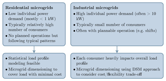
Figure 1.
Comparison of residential and industrial consumer characteristics in microgrids.
The flow chart in Figure 2 shows the steps of the proposed method. During data collection, the operation data of small industrial consumers are collected (A), and the local potential for power generation from RE sources is assessed (B). In the next step, scenarios are defined as combinations of different dimensioning steps of an MHP, a PV system, and a BESS (C). For each scenario, a generation profile (D), as well as system costs (E), are determined. The developed genetic algorithm is then applied to schedule all jobs of the consumers constrained by the power generation according to the consumers’ preferred operation times (F). We then evaluate the resulting schedules (G). Instead of interpreting them as exact operation schedules for the final microgrid, we use them to quantify the flexibility required from consumers. Together with the calculated Levelized Cost of Electricity (LCOE) (H), it is now possible to make a cost–flexibility trade-off compromising between electricity cost and required consumer flexibility (I).
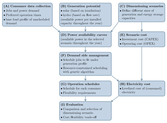
Figure 2.
Overview of the proposed microgrid dimensioning approach.
2.2. Consumer Data Collection
In this first step, the characteristics of potential electricity consumers in the microgrid are assessed. Each consumer can contribute scheduled and unscheduled loads to the total demand. Unscheduled loads are defined as an hourly load profile for one week.
Scheduled loads are represented by jobs that describe a shift of a given consumer. Table 1 shows the properties of a job.

Table 1.
Properties of jobs used in the scheduling algorithm.
A job is defined to have a constant power demand for a certain duration. This “rectangle” load profile is an obvious simplification of the actual load a small industrial consumer would have during a shift. For the purpose of the developed dimensioning method, it represents the power that needs to be available or “reserved” in the microgrid to ensure the operation of the consumer. Productive processes such as mills or workshops mainly use electric motors, which have start-up powers up to four times the nominal power lasting for a few milliseconds to seconds depending on the machine’s inertia [10]. Since it is unlikely that multiple motors in the microgrid are started exactly at the same time, it is tolerable that the motor’s start-up power exceeds the reserved power for a short time.
Consumers’ operating times can be specified for each hour of one day and by weekdays. The three categories shown in Table 2 represent the preferred times of operation.
Table 2.
Classification of operating times and their flexibility cost.
2.3. Renewable Generation Potential
Electricity generation from micro hydropower is defined by the available flow rate and hydraulic head. We only consider run-of-river type MHP without water storage. Therefore, the available flow rate directly impacts the power output of the MHP.
Solar irradiation at the site defines the local solar power potential. We use the Photovoltaic Geographical Information System (PVGIS) tool [43] to determine solar power output per kilowatt-peak installed capacity of a PV system. PVGIS uses a model to calculate PV power output considering air temperature, wind speed, cell technology, solar spectrum, and shallow-angle reflection, which is presented in further detail in the cited publications [44,45].
For the subsequent steps of the process, we calculate the multi-annual average of hourly generation potential of solar and hydropower.
2.4. Dimensioning Scenarios
Scenarios are defined by the combination of different sizings of system components of the microgrid. The dimensioning of the solar system and micro hydropower plant define how RE potentials are used and therefore define the power generation throughout the year.
At the same time, the investment and, therefore, the yearly cost of the microgrid depend on the dimensioning of its components. The yearly cost of the system is calculated using the annuity method as proposed in [46]:
Based on annual cost and annually delivered energy, the LCOE is calculated as follows:
2.5. DSM—Scheduling of Consumer Operation
The scheduling of consumer jobs is performed for each scenario. Based on the resulting operation schedules, the required consumer flexibility can be evaluated for each scenario. In the following, we describe the formulated resource-constrained scheduling problem to be solved with the implemented genetic algorithm.
2.5.1. Objective Function
The scheduling problem is solved by minimizing the following objective function, which is applied to evaluate the fitness of each individual of the population in the generational loop of the GA.
The objective function contains the decision variables shown in Table 3 to which an individual weight is assigned. The calculation of the value of the decision variables in the evaluation function of the implemented GA is described in Section 2.6.2.
Table 3.
Decision variables.
2.5.2. Constraints
The scheduling is carried out minimizing the objective function under the following constraints.
- Each job must be scheduled once within the timeframe defined by its release and deadline. This constraint is respected by the seeding and mutation function of the implemented GA. Therefore, populations always consist of individual solutions which respect this constraint.
- Jobs of the same consumer cannot be scheduled in parallel. Therefore, for valid scheduling solutions, the value of the decision variable parallel_schedule_hours must equal 0.
- The power demand of the scheduled jobs must be equal to or less than the availability at any timestep. The power availability at every timestep t is defined by the RE generation, the total unscheduled load, and the power provided by the BESS as follows:The power demand of the scheduled jobs at a given timestep t equalswith N being the number of consumers and being the power demand of a job of consumer n.The sum of excess power demand throughout the scheduling period equals the power_overshoot, which must be 0 for a valid scheduling solution.
- The power of the BESS at a given timestep t is positive when it is discharged and negative when it is charged. It is constrained by its capacity, C-rate, and SoC limits. A BESS model respecting these constraints is implemented in the GA. It is described in further detail in Section 2.6.2.
2.6. Implementation of the Resource-Constrained Scheduling Genetic Algorithm
We implemented a GA to solve the resulting resource-constrained scheduling problem using the Python library Distributed Evolutionary Algorithms in Python (DEAP) with the parameters shown in Table 4 [47].
Table 4.
Parameters used in the genetic algorithm.
2.6.1. Individual Representation
Each “individual” corresponds to a schedule of all jobs of the problem and is represented by a list of integer values. Its length is equivalent to the number of jobs to be scheduled. Each value represents the scheduled first timestep of the corresponding job, while the index represents the job’s ID. A seeding function creates the individuals of the initial population. It randomly selects starting times for each job, respecting the allowed timeframe defined by the job’s release and deadline.
2.6.2. Evaluation
During the evaluation, the fitness of an individual is determined. An operation schedule is created in which every job is placed according to the start time given by the individual. With this operation schedule and the power demand of each job, the resulting load profile of the individual is calculated. Based on the given power generation, the power overshoot—representing the “energy shortage per hour”—is calculated.
The BESS is modeled as a dispatchable load and generation capacity. The battery is charged when electricity generation exceeds the demand and discharged when the scheduled demand exceeds generation (see simplified sketch in Figure 3). The discharging and charging power of the BESS is limited by its specified C-rate as follows:
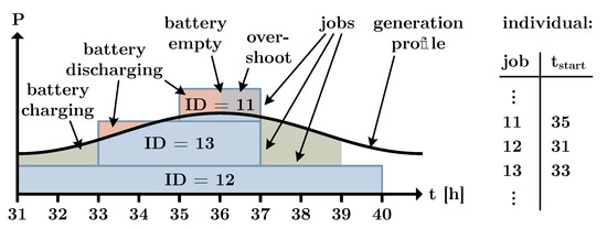
Figure 3.
Visual representation of the evaluation of individual fitness.
The evaluation function iterates through each timestep of the individual’s operation schedule. When the power availability at a given timestep exceeds the load of the scheduled consumer operation (), the battery is charged with the available excess power (). However, if the excess power exceeds the maximal charging power of the BESS () or the charging power required to achieve an SoC of 100% in the current timestep, the lower absolute value of the two is used as .
Any additional power that cannot be charged into the battery is automatically curtailed (i.e., not fed into the microgrid) and therefore is not part of the evaluation. In practice, a temporary surplus of energy in the electricity grid (compare timestep 39 in Figure 3) leads to a rise in frequency at which PV stand-alone inverters will gradually reduce their output power (not shown in the sketch). If the frequency continues to rise due to a then still existing surplus, the additional power is thermally dissipated by the electronic load controllers of the hydropower plant in order to maintain the power balance and stabilize the frequency.
In case the load of the scheduled consumer operation exceeds the available power (), the BESS is discharged with the required power to match the power overshoot (). If this power exceeds the maximal discharging power () or the maximal discharging power required to reach the lower bound of the BESS SoC defined by the maximum depth of discharge, the lower absolute value of the two is used for . The power overshoot at the given timestep is reduced by the according discharging power of the BESS.
Any additional power shortage that the battery cannot match will result in a power overshoot (), making the scheduling scenario invalid (compare timestep 36 in Figure 3).
Similarly, the number of hours of operation of jobs during unfavored and strongly unfavored hours and the parallel scheduling of jobs of one consumer are evaluated. The fitness of the individual is then calculated according to the objective function (5). Additionally, the evaluation function determines the contribution of every single job to the reduction of an individual’s fitness. The larger this contribution is, the higher is the probability of variation of the starting time of the job during mutation.
2.6.3. Selection
We use DEAP’s standard tournament selection with a tournament size of 3: The selection method randomly draws three individuals from the population and compares their fitness. The best individual of the ones drawn wins the tournament and is added to the offspring. This is repeated N times, with N being the number of individuals in the population.
2.6.4. Crossover
A two-point crossover is applied to two individuals in the offspring with a defined probability. The crossover exchanges a randomly drawn segment of the two individuals.
2.6.5. Mutation
The mutation function is applied to an individual with a user-defined probability. Each individual’s job starting time is varied with a probability defined by the job’s normalized fitness, which has been determined during evaluation. Therefore, jobs with a stronger negative impact on the individual’s fitness are moved with a higher probability. Similar to individual seeding, jobs can only be placed within their allowed timeframe (defined by release and deadline) during mutation.
3. The Case of Kalenge Industrial Campus on Idjwi Island, DR Congo
We apply the proposed method to the test case of the Kalenge Industrial Campus microgrid on Idjwi Island. The observations and exchange with the local operators of the campus were the motivation to develop the presented, novel method. In the following section, we introduce the test case. It is important to note that the collection of consumer data is preliminary and was completed remotely to generate a basis to test the method. A renewed, more detailed data collection is necessary for further application.
3.1. Site Background
Idjwi Island is located in the Eastern Democratic Republic of the Congo (DRC) in Lake Kivu at the border of Rwanda. As of 2017, it had an estimated population of 290,000, which was rapidly growing in the previous decade [48,49]. The lack of infrastructure is a major challenge. Energy access is scarce, since there is no public electricity grid with a connection to the mainland [49]. In the past years, off-grid electrification has gained some momentum, with several new microgrids being developed [50,51].
The Kalenge industrial campus is located on the eastern shore of the Island at GPS coordinates −2.0864, 29.0712. The local organization PROLASA developed the campus to provide infrastructure for small businesses to foster socio-economic development. An MHP with a maximum capacity of 20 kW was built to supply electricity for productive consumers such as corn mills, carpentry, welding, or coffee milling. Since the existing MHP only covers a fraction of the demand, it is planned to increase its capacity and potentially add a PV system to the microgrid. We demonstrate the proposed dimensioning method for the presented site with the system topology shown in Figure 4. The MHP includes an electronic load controller, which dissipates power when the generation exceeds the load.
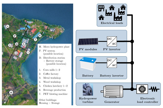
Figure 4.
Aerial image of the industrial campus with locations of generators and consumers (left), sketch of the assumed system topology (right).
The industrial campus currently uses a diesel generator to power larger consumers with a demand exceeding the power provided by the MHP. In a future energy system with increased RE generation capacities, the stakeholders aim to not depend on diesel generators due to the relatively high and volatile diesel price of 1.2 to USD/L (as of 2020) and difficult fuel supply and logistics.
3.2. Consumer Data
We collected data on energy consumers and their characteristics in interviews with the manager of the industrial campus and operators of individual businesses. The consumers listed in Table 5 were found to have scheduled operation, meaning they can adapt their operation to the available power generation. Their operation times and jobs have been specified as described in the Methods section.
Table 5.
Description of the scheduled consumers in the test case.
In addition, the base load profile of unscheduled energy demand at the industrial campus seen in Figure 5 was estimated based on the typical use of small electrical appliances and lighting observed on the industrial campus.
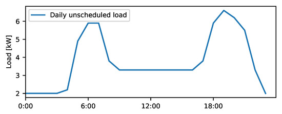
Figure 5.
Unscheduled load profile of the industrial campus.
3.3. Micro Hydropower Potential
The current MHP is located at the Tama River at GPS coordinates –2.09254, 29.06884, with a distance of approximately 800 m to the industrial campus. The potential intake for an extended, future MHP will be approximately 700 m upstream, providing a head of 120 m. These site specifications are defined by local circumstances, such as available land and accessibility. The Tama River has a catchment area of around 8 km2 at the potential intake position. Local flow rate measurements and modeled runoff based on GIS precipitation data [52] provide the estimated flow rate data depicted in Figure 6. A seasonal change between rainy and dry seasons can be observed.
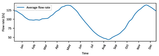
Figure 6.
Average available flow rate at the MHP site.
3.4. Solar Power Potential
The solar potential was evaluated using the PVGIS tool [43]. The potential output of a PV system in kW/kWp was determined with an hourly resolution from 2005 to 2016 as a basis to calculate a multi-year average power output. As shown in Figure 7, there are very small seasonal changes in the solar power availability at the site.
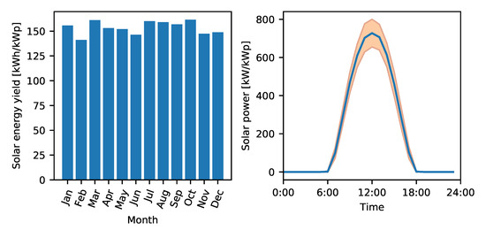
Figure 7.
Monthly solar energy yield at the microgrid site (left) with mean daily power curve and its standard deviation (right).
3.5. Techno-Economic Specifications of System Components
Table 6 summarizes the techno-economic specification of the considered system components. We assume a weighted average cost of capital (WACC) of 10%.
While being one of the most cost-effective off-grid electricity generation technologies, calculating the economic performance of MHP is challenging due to the strong dependency on site-specific factors [53,54]. Therefore, their cost can range from 2000 to 10,000 USD/kW depending on site characteristics. Generally, the cost of MHP per installed capacity decreases with higher hydraulic heads [55,56]. The following cost estimations for the site on Idjwi Island are based on reported cost per kW from MHP projects in neighboring Rwanda.
Table 6.
Techno-economic assumptions for the system components.
Table 6.
Techno-economic assumptions for the system components.
| Component | CAPEX | OPEX | Lifetime | Other Assumptions |
|---|---|---|---|---|
| MHP | 4000 [57] | 100 [58] | 40 a |
|
| PV system | 1600 | 15 [46] | 20 a [46,59] |
|
| BESS *4 | 900 | 10 [61] | 10 a [46,61] |
|
| Grid *6 | 110,000 USD | 2% | 20 a [64] |
*1 The efficiency includes all components of the MHP (penstock to generator) and is assumed to be constant. For the given hydraulic head, a Pelton turbine, which has high partial-load efficiency, would be most suitable [65]. *2 Estimation is based on the cost range given in [46,59]. *3 Optimal tilt in Rwanda is at -3°, but a steeper anglewas chosen to allow the rain to wash off dust [66]. *4 We only consider lithium-ion batteries since they havebecome the most economical battery technology for most microgrid applications [67]. *5 Estimated cost for the full AC-coupled battery system, including battery and inverter, based on cost range given in [46,62,67]. *6 These assumptions are based on cost data from the already existing distribution grid infrastructure at the site. For simplification, we assume no dependency on installed generation capacities.
3.6. Dimensioning Scenarios
We consider two “base scenarios” defined by the dimensioning of the MHP with 45 and 75 L/s nominal flow rate. Here, 45 L/s represents the base flow rate, which is available for at least 95% of the year and therefore provides a steady hydropower generation. At around 60% of the year, the available flow rate exceeds 75 L/s. This second MHP dimensioning scenario provides a higher annual energy supply at the cost of seasonal variations due to the rainy and dry seasons. The scenarios are defined by the combination of the dimensioning steps of each component, as shown in Table 7. We assume that scenarios including a PV system require a BESS for system stability and to account for short-term fluctuations of PV generation due to shading from clouds. Therefore, a total of 42 dimensioning scenarios are considered.
Table 7.
Overview of the dimensioning scenarios.
4. Results and Discussion
4.1. The Test Case of Kalenge Industrial Campus, Idjwi Island
We applied the developed method for the presented test case and the defined dimensioning scenarios. In the first step, the annual costs of the considered dimensioning scenarios are calculated based on the techno-economic parameters and the respective component sizing. We model a yearly power generation profile for each scenario combining the power output of the MHP and the PV system throughout the year based on the previously presented RE potential. The implemented algorithm is applied for each scenario to schedule the consumers’ jobs, minimizing the operation outside the consumers’ preferred operation times. Table 8 shows the selected parameters of the genetic algorithm.
Table 8.
Parameter values chosen for the genetic algorithm.
We conducted the scheduling on a computer with an i9-9900K CPU ( GHz) and 32 GB RAM, on which one generational loop took approximately 8.8 s per scenario. Figure 8 shows the convergence of the cost function of Equation (5) for the individual scenarios during the progress of the GA. After approximately 1500 generations, all scenarios show only slow improvements, and we assume convergence toward the respective optimum.
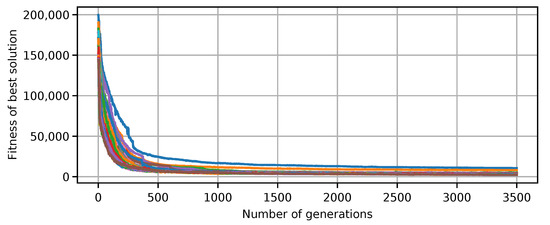
Figure 8.
Convergence of the fitness of the best solutions discovered for each scenario.
For each scenario, the algorithm returns the schedule of consumer operation of the best solution discovered. Figure 9 shows exemplary segments of resulting power demand after scheduling. The generation profile represents the maximal RE generation available before curtailment by the electronic load controller of the MHP or the PV inverter. The adaptation of demand to seasonally and daily varying generation is visible. The battery allows the demand to exceed the electricity generation for short periods.
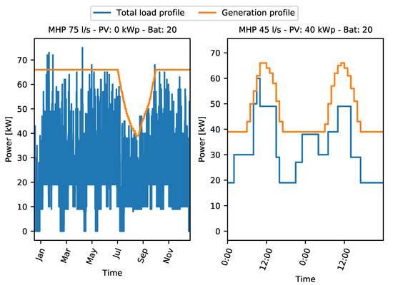
Figure 9.
Exemplary segment of load and generation profiles after scheduling for the whole year (left) and detailed view of one day (right).
As mentioned in Section 2.1, operation schedules are used as a basis to quantify how much consumer flexibility is required to fulfill the demand with the defined microgrid dimensioning scenarios. They are not intended to be used as exact, yearlong schedules for consumer operation once the off-grid system is completed. Instead, analyzing the modeled operation schedules in the dimensioning process provides insight into the required consumer flexibility during operation.
For example, base scenarios using only an MHP and no PV system or BESS show shifts of energy demand to night hours, indicating increased operation outside consumers’ preferred times. Further analysis of the resulting load profiles demonstrates this effect. The hourly profiles of average weekly load in Figure 10 show the increase of daytime peak and decrease of nighttime demand with increasing microgrid capacities for three exemplary scenarios.
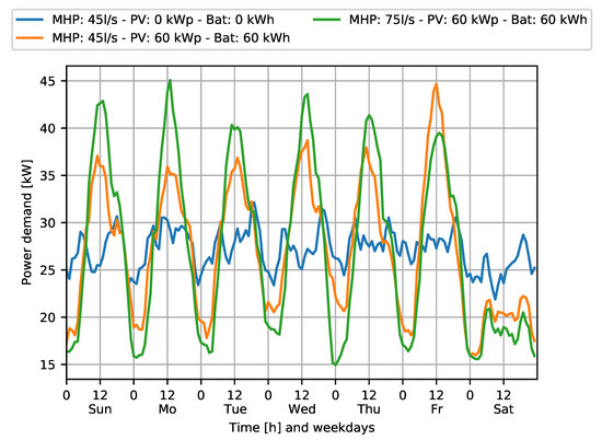
Figure 10.
Average week load profile of 3 exemplary scenarios.
A flatter load profile with higher nighttime operation means that a larger fraction of generated energy of the MHP is used. Therefore, smaller dimensioning scenarios have higher load factors which reduce LCOE at the cost of increasing required consumer flexibility.
Figure 11 shows this effect in detail for the beverage production in the test case. An increase in system component dimensions reduces operating hours outside of the preferred operation times. Visualizations such as this can help local stakeholders understand the impact of increased required flexibility on their operation.
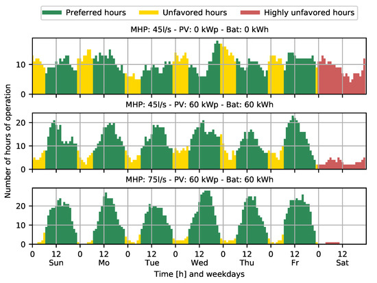
Figure 11.
Sum of operating hours of the beverage production for each hour of the week over the period of one year—three exemplary scenarios.
In order to quantify the overall consumer flexibility required for each scenario, we calculate the total number of hours of operation outside of the preferred operation times. LCOE is calculated based on the yearly delivered energy and the scenario’s annual cost.
Figure 12 and Figure 13 show that an increase in consumer flexibility can significantly decrease LCOE. For the test case on Idjwi Island, the modeled scenarios result in LCOE ranging from over 0.32 USD/kWh to just below 0.15 USD/kWh. Together with the analysis of the scheduling results, we can now quantify the relationship between required consumer flexibility and LCOE and use it as a basis for selecting a system design.
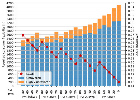
Figure 12.
LCOE and required consumer flexibility over decreasing system component dimensioning for the 45 L/s MHP base scenario.
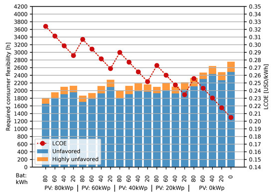
Figure 13.
LCOE and required consumer flexibility over decreasing system component dimensioning for the 75 L/s MHP.
The value or cost of consumer flexibility is subject to numerous locally specific, non-technical factors which can hardly be depicted in a microgrid dimensioning method. Therefore, we propose a manual selection and decision by the local stakeholders compromising between flexibility cost and LCOE. For example, the operator of a corn mill might be willing to start their morning shift at 6:00 instead of 8:00 to achieve an electricity price that allows them to operate economically. Productive users of energy should be able to decide how flexible they want to be to reduce their cost of energy.
The final selection of an optimal microgrid design for the test case should be based on further considerations. The MHP’s dimensioning can hardly be adapted cost-efficiently when the electricity demand grows in the following years, since civil works and hydro-mechanical equipment would have to be replaced. PV and BESS, on the other hand, could be expanded relatively easily. At the same time, with the estimated demand for the test case, LCOE values below USD/kWh are only achievable with the smaller MHP. Depending on the individual ability to pay of consumers and their willingness to operate flexibly, local stakeholders can make an informed decision for an economically viable off-grid energy system.
4.2. Uncertainties in Demand and RE Generation
The developed method determines the required consumer flexibility by scheduling the shifts of small industrial consumers constrained by the available RE generation. The number of shifts and, therefore, the total energy demand as well as the RE generation profiles are subject to uncertainties that impact the resulting required consumer flexibility.
While these uncertainties were not considered during the demonstration of the developed method with the test case, they can be addressed in a further application by varying the energy demand and RE generation in sensitivity analyses.
During consumer data collection, instead of recording a fixed number of jobs for each consumer, a range of the number of shifts can be determined, taking into account uncertainty and the possible development of energy demand. Uncertainty in RE generation can be represented by modeling generation profiles of single years instead of a multi-year average. Applying the developed method would then result in a possible range of required consumer flexibility.
4.3. Comparison with the Conventional Dimensioning Method
As previously described, conventional methods of microgrid dimensioning rely on modeled load profiles as a basis to design a cost-optimal energy system. For comparison, we apply this conventional approach for the test case using HOMER Pro. In the first step, a synthetic load profile is modeled. HOMER includes standard load profiles for different types of consumer characteristics. The “commercial” profile was selected as it fits best to the typical demand profile of the industrial campus. A random day-to-day variability and timestep variability of 10 and 20%, respectively, are applied to create a synthetic, yearlong load profile that is scaled to match the average daily energy demand of 653 kWh.
The load profile in HOMER (see Figure 14) shows significantly higher daytime loads than the results of the scheduling approach. While a more sophisticated load profile modeling of the industrial campus could be performed to consider the consumer characteristics in detail, it would still lack information on the required consumer flexibility.
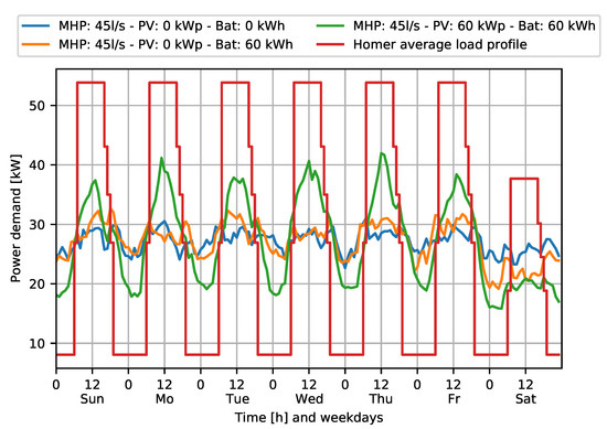
Figure 14.
Weekly average load profile of HOMER (red) together with results of the scheduling approach.
We optimized an off-grid energy system for the base scenarios of a 45 and 75 L/s MHP with the techno-economic parameters listed in Table 6 in Section 3.5 and obtained the results summarized in Table 9.
Table 9.
Results of the microgrid optimization with HOMER Pro.
We can now compare the resulting microgrid designs from HOMER Pro with the results of our novel method. For base scenario A, the resulting system dimensions are slightly larger than in the modeled scenarios. HOMER’s result for base scenario B lies in the middle of the range of the modeled scenarios.
In both cases, the scheduling results indicate that HOMER’s standard load profile would still require consumer flexibility. This is not quantified during system design and could therefore lead to problems and unanticipated shortages during microgrid operation.
HOMER’s results suggest a relatively large system design and high LCOE. The conventional approach does not allow compromising between consumer flexibility and LCOE in order to match the consumer’s ability to pay. While manually estimating a “flatter” load profile to optimize another scenario is possible and would likely reduce LCOE, the users would not know if the system was feasible for their demand and how much demand side flexibility it would require.
5. Outlook
The presented results for the test case demonstrated that the proposed method and algorithm provide a quantified insight into the trade-off between LCOE and required consumer flexibility in a microgrid for the productive use of energy. The results also point to numerous possible future improvements and further development to facilitate practical application.
5.1. Improved Definition of the Search Space
The current approach requires a search space, which is manually defined by the sizing steps of the system components. Therefore, it is possible to miss an optimal solution either because it lies outside the search space or between defined steps. A possible solution is to apply the developed method in a multi-step process in combination with the conventional dimensioning approach. In the first step, an optimization using a modeled load profile would be performed, as demonstrated in Section 4.3. The resulting microgrid capacities then define the upper limit of the search space for the DSM approach presented in this paper. After this first run, users can further limit the search space to an “area of interest”, where required consumer flexibility and LCOE are feasible. In this reduced search space, a further run of the DSM approach with smaller steps can be performed. Furthermore, the resulting load profile of a selected dimensioning scenario could be used to verify the results using a conventional dimensioning method.
5.2. Performance Improvements and Reduction of Complexity
The reduction of step size or the extension of the search space would again increase the problem size, which points to a limitation of the current implementation: Solving many relatively large scheduling problems is computationally expensive. It is unlikely that in practical applications, users would be willing to run multi-day optimizations to design an off-grid energy system. The current implementation of the GA shows potential for significant performance improvements, for example, from parallelization and parameter tuning. Reducing the modeled timeframe during optimization from one year to one exemplary month would significantly reduce the problem complexity. Modeling a full year gives the ability to take seasonal variations of generation and demand into account easily. While this is useful for the presented test case, where the hydropower generation shows seasonal variations, it might not be necessary in many other cases, especially in microgrids in Central Africa that rely only on solar power. Reducing the observed timeframe to exemplary segments would also likely reduce the complexity of consumer data collection.
5.3. Combination with Conventional Microgrid Dimensioning Methods Using Modeled Load Profiles
In practical application, our proposed method might be most beneficial in combination with conventional approaches to load profile modeling. A typical microgrid in the Global South, where anchor consumers act as enablers for rural electrification, could have a limited number of small industrial users and many residential consumers with little individual electricity demand [10,11]. The residential, unscheduled baseload can be modeled based on standard load profiles, while the cost of electricity for small industrial consumers could be reduced by finding a feasible compromise with the required flexibility.
5.4. Modeling Diesel Generators
Modeling dispatchable generation from diesel generators is another possible future improvement of the developed method. This would enable the application of off-grid systems with PV as the only RE generation technology, which often include diesel generators as backup. Exploiting demand side flexibility could prove especially valuable in solar–diesel microgrids where the use of the diesel backup generator is associated with high variable costs.
5.5. Incentive Models to Encourage and Reward Consumer Flexibility in Microgrids
The developed method gives users a quantified relationship between required consumer flexibility and the cost of electricity. This is a valuable basis for developing incentive and operation models for productive users of energy that motivate demand flexibility and reward contributions to reduced LCOE. In order to facilitate the stable operation of the microgrid and to avoid overloads, it might be necessary to include remote or timed switches in the microgrid, which connect and disconnect scheduled consumers according to previously agreed operating hours.
5.6. Further Application at the Test Case Site on Idjwi Island
We aim to further develop and apply the novel approach at the presented site on Idjwi Island. The discussion of our results with local stakeholders can provide valuable insight for future work. It is important to understand which analysis or visualization consumers need to assess and understand the implications of required flexibility for their operation to make an informed flexibility–LCOE trade-off.
Furthermore, a renewed consumer data collection at the site of the test case would be valuable to account for past changes as well as the possible future development of energy demand. At the same time, this gives the chance to develop reliable and efficient methods to collect the required structured consumer data, for example, in workshops or interviews with local stakeholders.
5.7. Microgrid Stability during Operation of Industrial Consumers
The productive use of energy in microgrids poses further challenges outside of the scope of economic system optimization. Industrial consumers such as mills often use asynchronous motors that can make up a significant share of the total load of the microgrid. Especially during start-up, this can be challenging for frequency and voltage stability. Investigating this effect and possible measures to reduce it is valuable, since it can impact the scheduling and operation of small industrial consumers.
5.8. Assessing Small Hydropower Potential for Off-Grid Energy Systems
Finally, the experience from the site on Idjwi Island has shown that while MHPs have a large potential in off-grid energy supply for the productive use of energy, there are significant challenges that complicate their development. Other than for solar power, a quick analysis of generation potential based on GIS data is difficult. Hydropower potential is heavily dependent on site-specific factors and flow rate data. Therefore, the further development of tools that evaluate MHP potential and their integration in dimensioning methods for off-grid energy systems could be a valuable contribution [68].
6. Conclusions
Decentralized electricity supply with microgrids is essential in achieving universal energy access, especially in rural regions in the Global South. Off-grid electrification using renewable energy sources gives rural communities energy independence and improves living conditions. The productive use of electricity in microgrids can ensure their economic viability and foster socio-economic development.
The dimensioning of off-grid energy systems defines their investment, operation, and energy cost. Therefore, appropriate sizing is a key factor for long-term success. Conventional dimensioning methods rely on modeled load profiles and entail uncertainty, especially in microgrids with a high share of productive users of energy. At the same time, they do not provide the opportunity to account for consumer flexibility and quantify its value in reducing LCOE.
In this paper, we present a novel method of microgrid dimensioning that aims to overcome these limitations. Instead of modeling load profiles, we represent the electricity demand of industrial consumers as flexible jobs that can be scheduled according to consumers’ preferences and available renewable energy. This method of applying demand side management during system design gives the opportunity to quantify the value of consumer flexibility to reduce LCOE.
We implemented a genetic algorithm to solve the resource-constrained scheduling problem. While the complexity of the scheduling problem makes it computationally expensive, it proves to be capable of finding viable solutions. We propose several further improvements of the algorithm and simplification of the problem to overcome this limitation.
We demonstrate the novel method with the test case of a microgrid that is planned to supply multiple small industrial consumers on Idjwi Island, DRC. The results show that consumer flexibility has a significant impact on the resulting energy cost. For the test case, LCOE ranging from 0.15 to 0.32 USD/kWh are possible depending on consumer flexibility. The quantified cost–flexibility trade-off gives local stakeholders the ability to make an informed compromise when designing an off-grid system that matches their ability to pay and the demand side flexibility they are willing to provide.
We compare the novel method with a conventional approach relying on a modeled load profile with HOMER Pro. With the resulting system design, an LCOE of approximately 0.26 USD/kWh is achieved. Unlike the proposed novel method, it does not provide insight into the potential to reduce LCOE by increasing demand side flexibility.
With the presented novel method, we overcome this limitation and contribute a new approach to designing economically viable microgrids for PUE.
Author Contributions
Conceptualization, J.K. and M.L.; methodology, J.K.; software, J.K.; validation, J.K.; formal analysis, J.K.; investigation, J.K.; resources, J.K. and M.L.; data curation, J.K.; writing—original draft preparation, J.K.; writing—review and editing, M.L.; visualization, J.K. and M.L.; supervision, M.L.; project administration, M.L. All authors have read and agreed to the published version of the manuscript.
Funding
The presented work was funded by the German Research Foundation (DFG) as part of the Research Training Group 2153: ‘Energy Status Data—Informatics Methods for its Collection, Analysis and Exploitation’.
Institutional Review Board Statement
Not applicable.
Informed Consent Statement
Not applicable.
Data Availability Statement
The presented data and developed software code are available at the following Git repository: https://git.scc.kit.edu/ipe-avt/dsm_mg_energies (accessed on 8 August 2022)—KITopen-ID: 1000151341. https://publikationen.bibliothek.kit.edu/1000151341 (accessed on 8 August 2022).
Acknowledgments
We acknowledge support by the KIT-Publication Fund of the Karlsruhe Institute of Technology.
Conflicts of Interest
The authors declare no conflict of interest. The funders had no role in the design of the study; in the collection, analyses, or interpretation of data; in the writing of the manuscript, or in the decision to publish the results.
Abbreviations
The following abbreviations are used in this manuscript:
| BESS | Battery Energy Storage System |
| CAPEX | Capital Expenditures |
| CRF | Capital Recovery Factor |
| DEAP | Distributed Evolutionary Algorithms in Python |
| DRC | Democratic Republic of the Congo |
| DSM | Demand Side Management |
| GA | Genetic Algorithm |
| GIS | Geographic Information System |
| ILP | Integer Linear Programming |
| LCOE | Levelized Cost of Electricity |
| MHP | Micro Hydropower Plant |
| MILP | Mixed-Integer Linear Programming |
| OPEX | Operating Expenses |
| PUE | Productive Use of Energy |
| PV | Photovoltaic |
| PVGIS | Photovoltaic Geographical Information System |
| RCSP | Resource-Constrained Scheduling Problem |
| RE | Renewable Energy |
| SDG | Sustainable Development Goal |
| SoC | State of Charge |
| UN | United Nations |
| WACC | Weighted Average Cost of Capital |
References
- IEA; IRENA; UNSD; World Bank; WHO. Tracking SDG 7: The Energy Progress Report; World Bank: Washington DC, USA, 2021. [Google Scholar]
- United Nations. Resolution adopted by the General Assembly on 25 September 2015, Transforming our world: The 2030 Agenda for Sustainable Development; United Nations Sustainable Development Summit 2015: New York, NY, USA, 2015. [Google Scholar]
- International Energy Agency. Energy Access Outlook 2017: From Poverty to Prosperity; IEA: Paris, France, 2017. [Google Scholar]
- Cader, C. Is a Grid Connection the Best Solution? Frequently Overlooked Arguments Assessing Centralized Electrification Pathways; Micro Perspectives for Decentralized Energy Supply (MES): Bangalore, India, 2015; pp. 137–141. [Google Scholar]
- Blechinger, P.; Köhler, M.; Jütte, C.; Berendes, S.; Nettersheim, C. Off-Grid Renewable Energies to Achieve SDG-7 and SDG-13: Cheaper, Cleaner and Smarter; Alliance for Rural Electrification: Brussels, Belgium, 2020. [Google Scholar]
- Blechinger, P.; Köhler, M.; Jütte, C.; Berendes, S.; Nettersheim, C. Off-Grid Renewable Energy for Climate Action—Pathways for Change; ’Deutsche Gesellschaft für Internationale Zusammenarbeit (GIZ) GmbH: Bonn, Germany; Eschborn, Germany, 2019. [Google Scholar]
- Mehta, R. A Microgrid Case Study for Ensuring Reliable Power for Commercial and Industrial Sites. In Proceedings of the 2019 IEEE PES GTD Grand International Conference and Exposition Asia (GTD Asia), Bangkok, Thailand, 19–23 March 2019; pp. 594–598. [Google Scholar] [CrossRef]
- Mandelli, S.; Barbieri, J.; Mereu, R.; Colombo, E. Off-grid systems for rural electrification in developing countries: Definitions, classification and a comprehensive literature review. Renew. Sustain. Energy Rev. 2016, 58, 1621–1646. [Google Scholar] [CrossRef]
- Corfee-Morlot, J.; Parks, P.; Ogunleye, J.; Ayeni, F. Achieving Clean Energy Access in Sub-Saharan Africa. Financ. Clim. Futur. Rethink. Infrastruct. 2019, 1–76. [Google Scholar]
- Booth, S.; Li, X.; Baring-Gould, I.; Kollanyi, D.; Bharadwaj, A.; Weston, P. Productive Use of Energy in African Micro-Grids: Technical and Business Considerations; National Renewable Energy Lab (NREL): Golden, CO, USA, 2018. [Google Scholar]
- Kurz, K. The ABC-Modell: Anchor Customers as Core Clients for Mini-Grids in Emerging Economies; Deutsche Gesellschaft für Internationale Zusammenarbeit (GIZ) GmbH: Bonn, Germany; Eschborn, Germany, 2014. [Google Scholar]
- Olk, H.; Mundt, J. Photovoltaics for Productive Use Applications: A Catalogue of DC-Appliances; Deutsche Gesellschaft für Internationale Zusammenarbeit (GIZ) GmbH: Bonn, Germany; Eschborn, Germany, 2016. [Google Scholar]
- Robert, F.C.; Sisodia, G.S.; Gopalan, S. The critical role of anchor customers in rural microgrids: Impact of load factor on energy cost. In Proceedings of the 2017 IEEE International Conference on Computation of Power, Energy Information and Commuincation (ICCPEIC), Melmaruvathur, India, 22–23 March 2017; pp. 398–403. [Google Scholar] [CrossRef]
- Blechinger, P.; Papadis, E.; Baart, M.; Telep, P.; Simonsen, F. What Size Shall It Be? A Guide to Mini-Grid Sizing and Demand Forecasting; Deutsche Gesellschaft für Internationale Zusammenarbeit (GIZ) GmbH: Bonn and Eschborn, Germany, 2016. [Google Scholar]
- Chatterjee, A.; Burmester, D.; Brent, A.; Rayudu, R. Research Insights and Knowledge Headways for Developing Remote, Off-Grid Microgrids in Developing Countries. Energies 2019, 12, 2008. [Google Scholar] [CrossRef]
- Mohseni, S.; Brent, A.C.; Burmester, D. Off-Grid Multi-Carrier Microgrid Design Optimisation: The Case of Rakiura–Stewart Island, Aotearoa–New Zealand. Energies 2021, 14, 6522. [Google Scholar] [CrossRef]
- Rahimian, M.; Iulo, L.D.; Duarte, J.M.P. A Review of Predictive Software for the Design of Community Microgrids. J. Eng. 2018, 2018, 5350981. [Google Scholar] [CrossRef]
- Hossain-McKenzie, S.; Reno, M.J.; Eddy, J.; Schneider, K.P. Assessment of Existing Capabilities and Future Needs for Designing Networked Microgrids; Sandia National Laboratories: Albuquerque, NM, USA; Lifermore, CA, USA, 2019. [Google Scholar]
- HOMER Pro. Available online: https://www.homerenergy.com/products/pro/index.html (accessed on 2 February 2022).
- Simpkins, T.; Cutler, D.; Anderson, K.; Olis, D.; Elgqvist, E.; Callahan, M.; Walker, A. REopt: A Platform for Energy System Integration and Optimization. In Proceedings of the ASME 2014 8th International Conference on Energy Sustainability collocated with the ASME 2014 12th International Conference on Fuel Cell Science, Engineering and Technology (Volume 2), Boston, MA, USA, 30 June–2 July 2014. [Google Scholar] [CrossRef]
- Deforest, N.; Cardoso, G.; Brouhard, T. Distributed Energy Resources Customer Adoption Model (DER-CAM) v5.9; Lawrence Berkeley National Lab.(LBNL): Berkeley, CA, USA, 2018. [Google Scholar] [CrossRef]
- Ciller, P.; Ellman, D.; Vergara, C.; Gonzalez-Garcia, A.; Lee, S.J.; Drouin, C.; Brusnahan, M.; Borofsky, Y.; Mateo, C.; Amatya, R.; et al. Optimal Electrification Planning Incorporating On- and Off-Grid Technologies: The Reference Electrification Model (REM). Proc. IEEE 2019, 107, 1872–1905. [Google Scholar] [CrossRef]
- Hoffmann, M.; Reiner Lemoine Institut (RLI). Offgridders. Available online: https://offgridders.readthedocs.io/ (accessed on 2 February 2022).
- Williams, N.J.; Jaramillo, P.; Campbell, K.; Musanga, B.; Lyons-Galante, I. Electricity Consumption and Load Profile Segmentation Analysis for Rural Micro Grid Customers in Tanzania; PES/IAS PowerAfrica; IEEE: Cape Town, South Africa, 2018; pp. 360–365. [Google Scholar] [CrossRef]
- Blodgett, C.; Dauenhauer, P.; Louie, H.; Kickham, L. Accuracy of energy-use surveys in predicting rural mini-grid user consumption. Energy Sustain. Dev. 2017, 41, 88–105. [Google Scholar] [CrossRef]
- Mandelli, S.; Brivio, C.; Moncecchi, M.; Riva, F.; Bonamini, G.; Merlo, M. Novel LoadProGen procedure for micro-grid design in emerging country scenarios: Application to energy storage sizing. In Proceedings of the 11th International Renewable Energy Storage Conference (IRES), Düsseldorf, Germany, 14–16 March 2017; Volume 135, pp. 367–378. [Google Scholar] [CrossRef]
- Llanos, J.; Saez, D.; Palma-Behnke, R.; Nunez, A.; Jimenez-Estevez, G. Load profile generator and load forecasting for a renewable based microgrid using Self Organizing Maps and neural networks. In Proceedings of the 2012 International Joint Conference on Neural Networks (IJCNN), Brisbane, Australia, 10–15 June 2012. [Google Scholar] [CrossRef]
- Espín-Sarzosa, D.; Palma-Behnke, R.; Valencia, F. Modeling of Small Productive Processes for the Operation of a Microgrid. Energies 2021, 14, 4162. [Google Scholar] [CrossRef]
- Cader, C.; Pelz, S.; Radu, A.; Blechinger, P. Overcoming data scarcity for energy access planning with open data—The example of Tanzania. Int. Arch. Photogramm. Remote Sens. Spat. Inf. Sci. 2018, 42, 23–26. [Google Scholar] [CrossRef]
- Mandelli, S.; Brivio, C.; Colombo, E.; Merlo, M. Effect of load profile uncertainty on the optimum sizing of off-grid PV systems for rural electrification. Sustain. Energy Technol. Assess. 2016, 18, 34–47. [Google Scholar] [CrossRef]
- Allee, A.; Williams, N.J.; Davis, A.; Jaramillo, P. Predicting initial electricity demand in off-grid Tanzanian communities using customer survey data and machine learning models. Energy Sustain. Dev. 2021, 62, 56–66. [Google Scholar] [CrossRef]
- Bustos, C.; Watts, D. Novel methodology for microgrids in isolated communities: Electricity cost-coverage trade-off with 3-stage technology mix, dispatch & configuration optimizations. Appl. Energy 2017, 195, 204–221. [Google Scholar] [CrossRef]
- Gomes, I.; Melicio, R.; Mendes, V.M.F. Assessing the Value of Demand Response in Microgrids. Sustainability 2021, 13, 5848. [Google Scholar] [CrossRef]
- Wu, C.; Mohsenian-Rad, H.; Huang, J.; Wang, A.Y. Demand side management for Wind Power Integration in microgrid using dynamic potential game theory. In Proceedings of the 2011 IEEE GLOBECOM Workshops (GC Wkshps), Houston, TX, USA, 5–9 December 2011; pp. 1199–1204. [Google Scholar] [CrossRef]
- Mehra, V.; Amatya, R.; Ram, R.J. Estimating the value of demand-side management in low-cost, solar micro-grids. Energy 2018, 163, 74–87. [Google Scholar] [CrossRef]
- Vahid, A.; Jadid, S.; Ehsan, M. Optimal planning of a multi-carrier microgrid (MCMG) considering demand-side management. Int. J. Renew. Energy Res. (IJRER) 2018, 8, 238–249. [Google Scholar]
- Nazemi, S.D.; Mahani, K.; Ghofrani, A.; Amini, M.; Kose, B.E.; Jafari, M.A. Techno-Economic Analysis and Optimization of a Microgrid Considering Demand-Side Management. In Proceedings of the 2020 IEEE Texas Power and Energy Conference (TPEC), College Station, TX, USA, 6–7 February 2020. [Google Scholar] [CrossRef]
- Awais, M.; Javaid, N.; Shaheen, N.; Iqbal, Z.; Rehman, G.; Muhammad, K.; Ahmad, I. An Efficient Genetic Algorithm Based Demand Side Management Scheme for Smart Grid. In Proceedings of the 18th IEEE International Conference on Network-Based Information Systems, Taipei, Taiwan, 2–4 September 2015; pp. 351–356. [Google Scholar] [CrossRef]
- Barth, L.; Ludwig, N.; Mengelkamp, E.; Staudt, P. A comprehensive modelling framework for demand side flexibility in smart grids. Comput. Sci.—Res. Dev. 2018, 33, 13–23. [Google Scholar] [CrossRef]
- Zhu, Z.; Tang, J.; Lambotharan, S.; Chin, W.H.; Fan, Z. An integer linear programming based optimization for home demand-side management in smart grid. In Proceedings of the 2012 IEEE PES Innovative Smart Grid Technologies (ISGT), Washington, DC, USA, 16–20 January 2012. [Google Scholar] [CrossRef]
- Liu, J.; Liu, Y.; Shi, Y.; Li, J. Solving Resource-Constrained Project Scheduling Problem via Genetic Algorithm. J. Comput. Civ. Eng. 2020, 34, 04019055. [Google Scholar] [CrossRef]
- Prinsloo, G.; Dobson, R.; Brent, A. Scoping exercise to determine load profile archetype reference shapes for solar co-generation models in isolated off-grid rural African villages. J. Energy S. Afr. 2016, 27, 11–27. [Google Scholar] [CrossRef]
- PVGIS Online Tool. 2019. Available online: https://re.jrc.ec.europa.eu/pvg_tools/ (accessed on 2 February 2022).
- Huld, T.; Amillo, A. Estimating PV Module Performance over Large Geographical Regions: The Role of Irradiance, Air Temperature, Wind Speed and Solar Spectrum. Energies 2015, 8, 5159–5181. [Google Scholar] [CrossRef]
- PVGIS—Data Sources and Calculation Methods. 2022. Available online: https://ec.europa.eu/jrc/en/PVGIS/docs/methods (accessed on 2 February 2022).
- Bertheau, P. Supplying not electrified islands with 100% renewable energy based micro grids: A geospatial and techno-economic analysis for the Philippines. Energy 2020, 202, 117670. [Google Scholar] [CrossRef]
- Fortin, F.A.; de Rainville, F.M.; Gardner, M.A.G.; Parizeau, M.; Gagné, C. DEAP: Evolutionary Algorithms Made Easy. J. Mach. Learn. Res. 2012, 13, 2171–2175. [Google Scholar]
- Thomson, D.R.; Hadley, M.B.; Greenough, P.G.; Castro, M.C. Modelling strategic interventions in a population with a total fertility rate of 8.3: A cross-sectional study of Idjwi Island, DRC. BMC Public Health 2012, 12, 959. [Google Scholar] [CrossRef]
- Jimenez-Redal, R.; Arana-Landín, G.; Landeta, B.; Larumbe, J. Willingness to Pay for Improved Operations and Maintenance Services of Gravity-Fed Water Schemes in Idjwi Island (Democratic Republic of the Congo). Water 2021, 13, 1050. [Google Scholar] [CrossRef]
- Equatorial Power Projects—DRC. Available online: http://equatorial-power.com/drc-2/ (accessed on 3 February 2022).
- Tacconelli, C. An Integrated Approach to Decentralised Renewable Energy Systems Planning for Developing Countries. Ph.D. Thesis, Sapienza Unversità Di Roma, Rome, Italy, 2020. [Google Scholar]
- Yamazaki, D.; Ikeshima, D.; Sosa, J.; Bates, P.D.; Allen, G.H.; Pavelsky, T.M. MERIT Hydro: A High–Resolution Global Hydrography Map Based on Latest Topography Dataset. Water Resour. Res. 2019, 55, 5053–5073. [Google Scholar] [CrossRef]
- Filho, G.L.T.; Dos Santos, I.F.S.; Barros, R.M. Cost estimate of small hydroelectric power plants based on the aspect factor. Renew. Sustain. Energy Rev. 2017, 77, 229–238. [Google Scholar] [CrossRef]
- Yetano Roche, M.; Ude, N.; Donald-Ofoegbu, I. True Cost of Electricity: Comparison of Costs of Electricity Generation in Nigeria. 2017. Available online: https://epub.wupperinst.org/frontdoor/deliver/index/docId/6932/file/6932_Costs_Electricity.pdf (accessed on 10 January 2022).
- Ogayar, B.; Vidal, P.G. Cost determination of the electro-mechanical equipment of a small hydro-power plant. Renew. Energy 2009, 34, 6–13. [Google Scholar] [CrossRef]
- Kishore, T.S.; Patro, E.R.; Harish, V.S.K.V.; Haghighi, A.T. A Comprehensive Study on the Recent Progress and Trends in Development of Small Hydropower Projects. Energies 2021, 14, 2882. [Google Scholar] [CrossRef]
- Geoffrey, G.; Zimmerle, D.; Ntagwirumugara, E. Small Hydropower Development in Rwanda: Trends, Opportunities and Challenges. In Proceedings of the IOP Conference Series: Earth and Environmental Science, Shanghai, China, 19–21 January 2018; Volume 133, p. 012013. [Google Scholar] [CrossRef]
- International Renewable Energy Agency (IRENA). Renewable Energy Technologies: Cost Analysis Series: Hydropower; International Renewable Energy Agency (IRENA): Abu Dhabi, United Arab Emirates, 2012. [Google Scholar]
- Reber, T.J.; Booth, S.S.; Cutler, D.S.; Li, X.; Salasovich, J.A. Tariff Considerations for Micro-Grids in Sub-Saharan Africa; National Renewable Energy Lab.(NREL): Golden, CO, USA, 2018. [Google Scholar] [CrossRef]
- Reich, N.H.; Mueller, B.; Armbruster, A.; van Sark, W.G.J.H.M.; Kiefer, K.; Reise, C. Performance ratio revisited: Is PR > 90% realistic? Prog. Photovoltaics Res. Appl. 2012, 20, 717–726. [Google Scholar] [CrossRef]
- Mongrid, K.; Viswanathan, V.; Balducci, P.; Alam, J.; Fotedar, V.; Koritarov, V.; Hadjerioua, B. Energy Storage Technology and Cost Characterization Report; Pacific Northwest National Lab.(PNNL): Richland, WA, USA, 2019. [Google Scholar]
- Zakeri, B.; Syri, S. Electrical energy storage systems: A comparative life cycle cost analysis. Renew. Sustain. Energy Rev. 2015, 42, 569–596. [Google Scholar] [CrossRef]
- Dhundhara, S.; Verma, Y.P.; Williams, A. Techno-economic analysis of the lithium-ion and lead-acid battery in microgrid systems. Energy Convers. Manag. 2018, 177, 122–142. [Google Scholar] [CrossRef]
- Nowbakht, A.; Ahrarinouri, M.; Mansourisaba, M. Presenting a New Method to Estimate The Remaining Life of Aerial Bundled Cable Network. In Proceedings of the 23rd International Conference on Electricity Distribution, Lyon, France, 15–18 June 2015. [Google Scholar]
- Zhang, Z. Pelton Turbines; Springer: Berlin/Heidelberg, Germany, 2016. [Google Scholar]
- Jacobson, M.Z.; Jadhav, V. World estimates of PV optimal tilt angles and ratios of sunlight incident upon tilted and tracked PV panels relative to horizontal panels. Sol. Energy 2018, 169, 55–66. [Google Scholar] [CrossRef]
- Lockhart, E.; Li, X.; Booth, S.S.; Olis, D.R.; Salasovich, J.A.; Elsworth, J.; Lisell, L. Comparative Study of Techno-Economics of Lithium-Ion and Lead-Acid Batteries in Micro-Grids in Sub-Saharan Africa; National Renewable Energy Lab.(NREL): Golden, CO, USA, 2019. [Google Scholar] [CrossRef]
- Müller, M.F.; Thompson, S.E.; Kelly, M.N. Bridging the information gap: A webGIS tool for rural electrification in data-scarce regions. Appl. Energy 2016, 171, 277–286. [Google Scholar] [CrossRef]
Publisher’s Note: MDPI stays neutral with regard to jurisdictional claims in published maps and institutional affiliations. |
© 2022 by the authors. Licensee MDPI, Basel, Switzerland. This article is an open access article distributed under the terms and conditions of the Creative Commons Attribution (CC BY) license (https://creativecommons.org/licenses/by/4.0/).