Use of Hybrid Photovoltaic Systems with a Storage Battery for the Remote Objects of Railway Transport Infrastructure

Abstract

The use of a grid-tied photovoltaic system with a storage battery to increase the power of objects of railway transport infrastructure above the limit on consumption from the grid with the possibility of energy saving is considered. The methods of analysis of energy processes in photovoltaic systems with a storage battery are used. They are added via the processing of archival data of power generation of a photovoltaic battery and computer modeling results. A technique of system parameter calculation to increase the power according to the given load schedule of the object at constant and maximum possible degree of power increasing is developed. The values of the average monthly generation of a photovoltaic battery at the location point of the object based on archival data are used. The principle of the control of power, consumed from the grid, according to the given values of the added and total load is developed. Using the basic schedule of added load power in connection with the graph of photovoltaic battery generation allows reducing the installed power of the storage battery. The additional reduction in the installed power of the photovoltaic and storage batteries is possible at the corresponding choice of the degree of power load increasing. The joint formation of current schedules with reference to the added power value and state of charge of the battery according to the short-term forecast of the generation of a photovoltaic battery is proposed. The value of added power at certain intervals of time is set according to the graph of actual generation of the photovoltaic battery, which contributes to the maximum use of its energy. With the average monthly generation of a photovoltaic battery in the spring–autumn period, the discharge of the battery during the hours of the morning load peak is not used. This reduces the number of deep discharge cycles and extends the battery life. The description of energy processes in steady-state conditions for the daily cycle of system functioning is formalized. On this basis, a mathematical model is developed in MATLAB with an estimation of the costs of electricity consumed from the grid. When modeling, archival data are used for days when the generation of a photovoltaic battery over time intervals is close to average monthly values. This makes it possible to evaluate the effectiveness of system management under conditions close to real during the year.

1. Introduction

Photovoltaic systems (PVSs) are the most common in the “green” energy sector. A considerable share of PVSs falls on local objects (LO) for various purposes, where hybrid solar power plants with connection to the alternating current distribution grid (DG) are used. This corresponds to the current trend of localizing consumption at the generation site [1].

The issue of localization of the consumption of energy, generated by PV, can be solved when using a PVS to increase the load power of the LO above the limit on consumption from the grid. Such an application of PVS can be in demand during the development (expansion) of facilities with an increase in consumption, when the possibilities of increasing the capacity of the existing connection to the power grid are exhausted.

PVS application can be useful for railway infrastructure facilities remote from the transformer substation, including those with the seasonal nature of the load (consumption). The simplified structure of the power supply of LO with a PVS and storage battery (SB) is shown in Figure 1. The implementation of this option may be cheaper than laying a new power transmission line and replacing DG equipment. The advantage of this solution is the possibility of reducing the cost of paying for consumption from the DG during the term of operation of the PVS and the possibility of autonomous operation in the case of DG disruptions.

This also applies to objects of extensive railway transport infrastructure, including remote objects on sections of the grid that are not currently electrified. The main task when using PVS for such facilities is to provide for their own needs. At the same time, the possibility of increasing their power when using existing DG is limited by the consumption limit. The issue of energy saving remains relevant. First of all, this concerns the reduction in electricity consumption from DG. The use of storage batteries in the PVS with modern methods of energy management [2] allows rationally redistributing the energy in the system in time. This also achieves a reduction in consumption from DGs and an increase in the reliability of the power supply of LO. Improving the performance of systems with renewable sources of electricity is an urgent task, which contributes to the further development of energy with distributed sources of electricity.

2. Literature Review and Problem Statement

The demand for the use of hybrid PVS with SB is confirmed by the fact that the electrical market is widely represented by various solutions of hybrid inverters [3,4], which are designed for LO. They have all the equipment for connecting a photovoltaic battery (PV) and SB, as well as sufficiently powerful software. They are designed for self-consumption of LO while reducing consumption from DG, and they provide an uninterruptible power supply function.

With a power consumption of LO in excess of 10 kW, it is advisable to use three-phase multifunctional inverters while maintaining a power factor close to 1 at the point of common coupling (PCC) to the grid [5,6,7,8,9,10,11,12]. This allows to unload the grid from reactive power and ensures the symmetry of loading the phases of the grid at an unbalanced load [9,10,11,12]. A previous study [13] presented a three-phase PVS with an SB with four converters with a common link of direct current (DC). In the DC link, a proportional–integral (PI) voltage controller (VC) was used. The controller set the currents of the battery and supercapacitor. The “multiconverter” provided a given active power with the proper quality of electricity, PV operation with tracking the maximum power point (MPPT), and extended battery life with hybrid storage. In [10,11], the structure of the control system of a multifunctional inverter of a PVS with an SB with voltage stabilization in the DC link with three VCs was considered. The VC controls the currents of the SB and PV, as well as current in the PCC. The structure changes in accordance with the mode of operation, and only one of the VCs is always used. Ensuring the efficiency of the use of hybrid PVS with energy storage for LO is usually associated with a reduction in the cost of consuming electricity from the grid and an increase in the reliability of the power supply [14]. With a wide range of changes in PV generation during the year, cost reduction is achieved by overestimating the power of PV relative to the load power. This allows providing acceptable indicators in cloudy weather and winter.

PV generation changes significantly during the day and year. Therefore, the increase in the efficiency of PVS energy management is associated with the use of the forecast of PV generation [15,16,17,18,19]. The issues with obtaining an accurate forecast were considered in a number of studies, particularly [15,16]. Recently, web resources have been made available that provide a forecast with a discreteness of 0.5 h or less, including an individual one at the location [20,21]. For the application without generation to the grid, the main purpose of the forecast is load planning for the next day and the possibility of adjustment when it changes [19].

Certain opportunities to reduce the cost of paying for electricity consumed by LO from DG are provided by taking into account the tariffication of payment [19,22,23,24,25]. Features of the implementation of PVS in the application of static and dynamic tariffs were considered in [22].

When using PV for the needs of LO (without generating electricity to the grid), it is achievable to reduce the cost of electricity consumption from DG by up to five times at one tariff rate (up to seven times at wo rates) in the summer [19,26]. In winter, the reduction is insignificant—around 1.2 times. A general estimation of cost reduction for the year is not given. In [27], along with meeting the needs of the LO, the use of the planned generation of electricity in the grid during peak hours was considered. This allowed significantly reducing electricity costs. Overall estimation of cost reduction during the year was not given. Regardless, there was still an underutilization of PV energy in the summer.

An effective tool for assessing the efficiency of the energy management of a PVS with an SB is mathematical modeling [26,27,28,29]. Modeling of a hybrid system with a supercapacitor for the PV generation period was considered in [29]. Modeling of energy processes in the daily cycle with an estimate of the cost of paying for electricity consumed from the DG was considered in [26,27]. The use of archival data on PV generation [30] allowed studying the operation of the system in different weather conditions with an estimation of the cost of electricity, consumed from the DG.

The possibilities of PVS use for power increase for infrastructure objects, remote from the transformer substation, over the limit of consumption have not been sufficiently studied. This is related to the determination of parameters and limiting capabilities in different seasons of the year, the features of the formation of the SB state of charge in the process of operation, and the realization of the principles of added power formation at maximum use of PV energy. In this case, it is possible to reduce the installed power of the PV and the battery. An important role in assessing the capabilities of the system is performed by mathematical modeling.

Thus, the purpose of the article is to develop principles for the use of PVS with SB to increase the power of the LO above the power limit for consumption from the grid with the maximum use of PV generation.

The main objectives of the research are as follows:

-

to study the possibilities of increasing the load power of the LO above the power limit for consumption from the grid during the year;

-

to justify the choice of PVS parameters with the formation of the graph of added power according to the accepted load schedule of the LO with a decrease in the installed power of the PV and battery;

-

to develop principles for the implementation of the management of PVS using the forecast of PV generation;

-

to perform an assessment of the system’s capabilities in the daily mode for different seasons of the year using mathematical modeling.

3. Methodology of Research

A study of ways to improve the control mechanism of the PVS with an SB for increasing the power of the LO was carried out on the basis of analytical methods in electrical circuits. The results of processing statistical data on the PV generation for a given point of location of the object were also used. A proportional increase in power to the original load schedule was adopted. As original, the load schedule characteristic of objects with a predominance of day loads, with peak loads in the morning and evening and a decrease in the load at night, was considered. The basic schedule of power, added and provided by the PVS, was adopted in accordance with the PV generation schedule. The maximum value of the power increase factor in winter takes into account the possibility of ensuring the battery charge within the power limit for consumption from the grid. On this basis, the energy capacity of the battery was determined, followed by an assessment of the possibilities for increasing the load power, taking into account the average monthly PV generation. The choice of a fixed value of the degree of power increase was carried out while taking into account the use of PV energy and cost reduction. The control system of the PVS converter unit was implemented on the basis of a classic double-loop structure with voltage stabilization in the DC link. When forming the SOC(t) (state of charge) of the SB schedule, a limit of DOD ≤80% (depth of discharge) was introduced with one deep discharge per day in the spring–summer–autumn period. The technique to calculate the reference of added power for maximum use of PV energy was realized on the basis of an analysis of the average monthly PV generation by time intervals for the taken load schedule. Analysis of energy processes in the system “DG–PVS with SB–LO load” was carried out for the daily cycle without taking into account transient processes and higher harmonics in energy converters. Energy losses were accounted for through efficiency. The properties of the SB were considered in accordance with the characteristics of the manufacturer. PV generation was estimated on the basis of monthly average values for given time intervals during the day. Data of PV generation were obtained for the location point of the object when processing archival data for 5 years. The modeling of energy processes was performed using MATLAB software package using real archive graphs of PV generation. The days were chosen when PV generation by time intervals was close to the average monthly values. The model was completed on the basis of analytical expressions for steady-state operating modes, which correspond to generally accepted proven calculation methods. When the operating modes of the system changed, the corresponding calculated expressions were used at time intervals per day.

4. The Results of the Research on the Use of PVS with SB to Increase the Power of LO

The option of PVS with an SB with a grid multifunctional inverter VSI (Figure 2) was considered. The middle pin (n) of the VSI link DC was connected to the neutral connection point of the DG. This allowed ensuring the equalization of power consumption from the grid by phases under unbalanced load LO [9,10,11]. This also made it possible to control the active power P_g in the PCC. The structure of the PVS included the following elements: a DC voltage converter PV (CPV) with a transistor key for measuring the current of the PV short-circuit [10], and a DC voltage converter battery (CSB). The converter unit was controlled by a control unit (CU) connected to the programmable control unit (PCU). Communication with the web resource to obtain forecast data was provided by a Wi-Fi WFM module.

When solving the issue of increasing the power of the LO, the general approach changes somewhat; the DG becomes an auxiliary source of energy of limited power. As originally proposed, the use of a load schedule was considered in accordance with the standard distribution of peak loads [19,26] for objects of the utility sector and the nondomestic sector with a single-shift mode of operation. The following distribution of load intervals was accepted: night tariff zone in the period May–August (t₇ = 24.00, t₁ = 7.00), day tariff (t₁ = 7.00, t₂ = 8.00), (t₃ = 11.00, t₅ = 20.00), (t₆ = 23.00, t₇ = 24.00), peak load zones (t₂ = 8.00, t₃ = 11.00), and (t₅ = 20.00, t₆ = 23.00); in the period autumn–winter–spring (t₁ = 7.00, t₂ = 8.00, t₃ = 10.00, t₅ = 17.00 and 18.00, t₆ = 17.00 and 18.00, t₇ = 24.00). An additional point of time t₄, was also used, corresponding to the transition to an evening decrease in PV generation. This time during the year varied from t₄ = 16.00 in June to t₄ = 14.00 in December.

Increasing the power of the LO load in the daytime assumes that the total power P_LC of the LO load is defined as P_LC = P_Lg + P_C (where P_Lg is the power which is provided by consumption from the grid (P_Lg does not exceed the limit on consumption P_LIM), and P_C is the added power, generated by the inverter due to the energy of PV and SB). We can take P_Lg = P_LIM; then, with an increase in P_L; the possible value of P_LC grows with constant consumption from the grid. If the actual load power is less than P_LC, the electricity consumption from the grid is reduced.

The value of the energy generated by PV during the year varies widely (

Table 1. Average monthly PV generation during the year.

January	February	March	April	May	June	July	August	September	October	November	December
Average monthly generation of PV per day for Kyiv location WPVAVD, kWh
1.17	1.81	2.87	3.88	4.27	4.43	4.38	4.24	3.85	2.57	1.14	0.91
Average monthly generation of PV per day for Žilina location WPVAVDZ, kWh
1.272	2.053	2.811	3.799	3.76	3.914	4.073	3.84	3.434	2.6	1.418	1.25
Energy values for selected days when the PV generation was close to the average monthly generation per day in Kyiv (PV generation calculated using archival data for the period 2012–2016) W*PVAVD, kWh
0.85 (0.98)	1.81 (1.81)	2.57 (2.83)	3.89 (3.83)	4.25 (4.26)	4.47 (4.48)	4.36 (4.37)	4.036 (4.16)	3.4 (3.52)	2.44 (2.49)	0.798 (0.96)	1 (1.03)
Energy values for selected days when the PV generation is close to the average generation at time interval (t2, t3) in Kyiv (PV generation calculated using archival data for the period 2012–2016) WPV23, kWh
0.144 (0.166)	0.31 (0.36)	0.5 (0.55)	0.62 (0.52)	1.06 (1.15)	1.26 (1.17)	1.17 (1.13)	0.581 (1.08)	0.41 (0.56)	0.34 (0.33)	0.225 (0.22)	0.166 (0.21)
Energy values for selected days when the PV generation is close to the average generation at time interval (t3, t4) in Kyiv (PV generation calculated using archival data for the period 2012–2016) WPV34, kWh
0.643 (0.78)	1.31 (1.36)	1.83 (1.84)	2.09 (2.38)	2.43 (2.43)	2.51 (2.27)	2.46 (2.5)	2.78 (2.45)	2.25 (2.27)	1.95 (1.74)	0.535 (0.69)	0.806 (0.8)
Energy values for selected days when the PV generation is close to the average generation at time interval (t4, t5) in Kyiv (PV generation calculated using archival data for the period 2012–2016) WPV45, kWh
0.061 (0.038)	0.16 (0.083)	0.22 (0.32)	0.79 (0.84)	0.539 (0.53)	0.62 (0.63)	0.57 (0.61)	0.66 (0.53)	0.65 (0.72)	0.148 (0.39)	0.036 (0.03)	0.03 (0.021)

). Table 1 shows the data [30] on the average monthly generation of PV per day W_PVAVD at power P_PVR = 1 kW for the Kyiv location: latitude (decimal degrees)—50.451, longitude (decimal degrees)—30.524. Similar data are given for the city of Žilina W_PVAVDZ (latitude (decimal degrees)—49.224, longitude (decimal degrees)—18.748). In winter, the PV generation in Žilina is slightly higher. In Table 1 (in parentheses), monthly energy values per day (W*_PVAVD) and at time intervals during the day (W_PV23, W_PV34, and W_PV45) are also presented for Kyiv. The energy values without parentheses correspond to the selected days when the generation was close to the monthly average. These values were obtained from archival data of P_PV generation in Kyiv [30] for the period 2012–2016.

The value of the added load power P_C was determined on the basis of the average monthly daily generation of W_PVAVD ≈ 2500 W in the transitional seasons of the year (Table 1): October and March. In November–February, the load, provided by PV, decreased. The average value of power in the daytime (P_AVD = W_PVAVD/t_D, where t_D is the length of the day) was about 200 W.

We took the basic load schedule (average P_L values by time intervals) taking into account peak loads in the morning and evening with a decrease in load after t₄ until the evening peak, e.g., P_L23B = 200 W (P_LAVD), P_L34B = 180 W (0.9 P_LAVD), P_L45B = 160 W (0.8 P_LAVD), and P_L56B = 200 W (P_LAVD). The total night load of LO could be taken from the condition P_Lg62 = P_LIM − P_B (we took P_LIM equal to the peak power P_LIM = P_L23B = 200 W, P_B = U_BI_B—power, consumed from the grid to charge the SB (U_B and I_B—voltage and current of the SB)). At the same time, P_Lg62 ≥ P_LMIN, P_LgMIN = 0.2P_L56 in summer, and P_LgMIN = 0.3P_L56 in winter. The total energy transmitted by the inverter to increasing power (P_L) at the interval (t₂, t₆) was W_L26 = 2740 Wh in summer, W_L26 = 2580 Wh in autumn–spring, and W_L26 = 2410 Wh in winter.

The effective use of the SB’s capabilities for the redistribution of energy in the system involves the formation of the SOC(t) dependency $Q_{}^{\ast }\left(t\right)$ ($\hspace{0.17em}{Q}^{\ast }=100Q/Q_R$, $Q=Q_0+{\displaystyle \int I_{B}dt}$, $Q_R$ = C_B—the rated value (100%) or capacity (Ah) of the battery, $Q_0$—the initial value). Increasing the power during peak hours in the morning and evening, when the PV generation is small, implies a deep discharge of the SB. That is, we have two deep discharges per day. In these conditions, the use of lithium-ion batteries is preferable.

Two variants of implementation were considered: (1) with a maximum increase in power in accordance with PV generation, which is available for the consumers with seasonal load; (2) with a constant increase in power during the year.

For variant (1), it was assumed that the planning of load using the day-ahead forecast was possible.

For calculation of the value of SB energy capacity, in the interval (t₄, t₆), the PV generation W_PV45 is small, and the increase in power is achieved mainly due to the energy of the SB. At the same time, the energy balance is determined by the following expression:

$$0.01\cdot \Delta Q_{46}^{\ast }{W}_B\cdot {\eta }_C\cdot {\eta }_B=P_{C45}(t_5-t_4)+P_{C56}(t_6-t_5)-W_{PV45}\cdot {\eta }_C,$$

(1)

where W_B is the SB energy capacity (W_B = U_BC_B), $\Delta Q_{46}^{\ast }=Q_4^{\ast }-Q_6^{\ast }$, η_C is the general efficiency of the SB voltage converter and grid inverter, and η_B is the efficiency of the SB.

W_B is calculated from the condition of the functioning of the added power of the load during the evening peak hours (t₅, t₆) and on the intervals (t₄, t₅), when PV generation is significantly reduced. This is most typical in winter, with a longer evening peak (4 h). The limitation is to ensure the possibility of the battery charge and the operation of the load at night within the framework of P_LIM. When W_PV46 = 0, the value of the energy capacity of the battery SB is

$$W_B=\frac{W_{C46}}{0.01\cdot \Delta Q_{46}^{*}\cdot {\eta }_C\cdot {\eta }_B},$$

(2)

where W_C46 = W_L46 (ρ − 1); ρ > 1 indicates the degree of increase in the load power.

It was assumed that the night load in winter also proportionally increases P_Lg = ρ 0.3 P_LIM. The possible value for the battery charge in the framework of limit is denoted as

$$\Delta W_{B62}=(t_2-t_6)P_{LIM}(1-0.3\rho ).$$

(3)

Alternatively,

$$\Delta W_{B62}=\frac{W_{L46}(\rho -1)\Delta Q{*}_{62}}{\Delta Q{*}_{46}{({\eta }_C\cdot {\eta }_B)}^2}.$$

(4)

The maximum value ρ_MAX in the interval (t₄, t₆) can be determined in accordance with Equations (2) and (3). In this case, at DOD₆ ≤ 80%, ρ_MAX = 1.721. Accepting ρ = 1.7, W_B = 1164 Wh. At DOD₆ ≤ 90%, the value is W_B = 1034 Wh. The average value W_B = 1099 Wh (corresponding to, for example, C_B = 43 Ah at U_B = 25.6 V) can be accepted. The resulting value is sufficient to ensure the added power at ρ_MAX = 1.7 and average monthly PV generation in December in the interval (t₂, t₆).

However, for the same value P_LC = ρP_L and P_Lg ≤ P_LIM, the different variants of reference of the added power P_C for the interval (t₂, t₆) (in

Table 2. Variants of the reference P_C and P_Lg at ρ = 1.7.

	Interval	(t2, t3)	(t3, t4)	(t4, t5)	(t5, t6)
Variant	PLC, W	340	306	272	340
va	PC, W	140	126	112	140
	PLg, W	200	180	160	140
vb	PC, W	140	106	72	140
	PLg, W	200	200	200	200
vc	PC, W	140	200	72	140
	PLg, W	200	106	200	200

, data are presented for ρ = 1.7) are possible. This allows planning P_C(t) according to the conditions.

Above the variant, va was considered. At minimal PV generation (in winter), variant vb ensured the biggest value ρ, whereby P_C26(t) = ρP_L26(t) − P_LIM. In this case, W_C46 = ρW_L46 − P_LIM(t₆ − t₄), and the value ΔW_B62 can be expressed as

$$\Delta W_{B62}=\frac{P_{LIM}(6\rho -(t_6-t_4))\Delta Q{*}_{62}}{\Delta Q{*}_{46}{({\eta }_C\cdot {\eta }_B)}^2}.$$

(5)

We get values ρ_MAX = 1.78 and W_B = 968 Wh (corresponding to, for example, C_B = 37.8 Ah at U_B = 25.6 V). The advantage of this variant is the minimal value of P_C in the interval (t₄, t₆) when the PV generation is minimal.

Variant vc is included in Table 2. This variant is more tied to the PV generation schedule during the day.

There are days in winter when W_PVD ≤ 60 Wh. In this case, it is possible to use a night charge of the battery up to 100%, followed by a discharge during the day (from 8:00 a.m. to 9:00 p.m.) at DOD₆ = 10%. This allows using the energy ΔW_B26 = 768 Wh (at W_B = 968 Wh) in the load. Accordingly, ρ = (ΔW_B26 + W_L26LIM)/W_L26LIM = 1.3. At small values of W_PVD (for example, at W_PVD ≤ 300 Wh), there is the possibility to redistribute the energy of SB by intervals. For example, the degree of increase in power in peak hours can be saved without increasing from 10:00 a.m. to 5:00 p.m. Then, for example, 0.3 ΔW_B26 can be used in the morning peak, and, taking into account the duration, 0.6ΔW_B26 can be used in the evening peak. This allows ensuring ρ ≈ 1.6 in intervals (t₂, t₃) and (t₅, t₆).

In the period spring–autumn, there is the possibility to increase ρ. Determination of ρ is carried out in the accordance with forecast data of PV generation on the next day on the basis of the balance of energy in the intervals (t₂, t₆) and (t₄, t₆).

It is possible to calculate ρ for the interval (t₂, t₆) as follows:

$${\rho }_{26}=\frac{W_{PV26}{\eta }_C+\Delta W_{B26}-W_{gR26}+P_{LIM26}}{W_{L26}},$$

(6)

where W_gR26 indicates a decrease in energy consumption from the grid, and $W_{LIM26}=P_{LIM}(t_6-t_2)$.

Depending on the PV generation, the implementation is possible (a) with the discharge of the SB without a decrease in consumption from the grid, (b) without the discharge of the SB and a decrease in consumption from the grid, (c) with minimal discharge of the SB and a decrease in consumption from the grid, or (d) without the discharge of the SB and a decrease in consumption from the grid. Variant (a) is specific to winter with small PV generation, when ρ_MAX = 1.7 is accepted.

For interval (t₄, t₆),

$${\rho }_{46}=\frac{k{W}_{PV46}{\eta }_C+\Delta W_{B46}-W_{gR46}+P_{LIM46}}{W_{L46}},$$

(7)

where k is a coefficient, taking into account the use of PV energy for consumption, and ΔW_B46 corresponds to DOD = 80%.

The value of k takes into account that, when the SB is fully charged by the time t₄, only part of the PV energy is used for consumption by the load. The rest of the energy provides a reduction in consumption from the grid. Thus, k = 1 is accepted if W_PV45 · η_C < W_C45, while k = 0.5 is accepted if W_PV45 · η_C ≥ W_C45.

Furthermore, ρ₄₆ can be defined at the decrease in consumption in Equation (6) when W_gR46 = 0. For March (Table 1), ρ₄₆ = 1.8. Compared with the value ρ₂₆ = 2.02 according to Equation (6) for option (b), we accept the smaller value. In this case, with ρ = 1.8, it is possible to implement option (c). Thus, for ρ = 1.8, we find the following value:

$$\Delta Q{*}_{23}=\frac{W_{PV23}{\eta }_C-W_{C23}}{0.01W_B{\eta }_C{\eta }_B}.$$

(8)

For March ΔQ*₂₃ = 17% > 0, i.e., the SB state of charge increases, and the night battery charge is not needed. Then, in accordance with Equation (6), we have a decrease in consumption on the order of 572 Wh. With the average monthly values of PV generation for the summer period, ρ = 1.95 is achievable.

A graph of the added power P_C(t) and the state of charge of the SB Q*(t) is presented in Figure 3 in accordance with the obtained value of ρ. We consider options vb and vc when using the PV energy W_PV forecast data over time intervals. At the same time, it is desirable to (1) use the lowest possible power consumption at night (until 8:00 a.m.) per battery charge, and (2) ensure the condition Q*₄ → 100%, taking into account the reduction in PV generation in the evening. A prerequisite is the maximum use of PV energy.

Reference to the initial value Q*_2R is carried out in accordance with values ΔQ*₂₃ and ΔQ*₂₄ (calculated similarly to Equation (8)). If ΔQ*₂₄ ≤ 0, then Q*_2R = 100% (curves 1, 5, and 6 in Figure 3). In this case, when ΔQ*₂₄ > 0 and ΔQ*₂₃ ≤ 0, then Q*_2R = (100 − ΔQ*₂₄) ≥ 40% (curve 2 in Figure 3). If ΔQ*₂₄ > 0, ΔQ*₂₃ > 0, and W_PV23 · η_C/W¹_C23 < 1.5 (W¹_C23 is the value for the basic schedule with given ρ), then Q*_2R = (100 − ΔQ*₂₄) ≥ (Q*₆ + δ) (curve 3 in Figure 3, δ = 10–15%). In all cases, the reference of the added power is P_C23 = P¹_C23.

If ΔQ*₂₄ > 0, ΔQ*₂₃ > 0, and W_PV23 · η_C/W¹_C23 ≥ 1.5, then P_LC23 ≥ (P_C23 = P_PV23 · η_C) ≥ P¹_C23, which is given in accordance with PV generation. In this case, the SB charge (curve 4 in Figure 3) is not carried out. It also does not use the battery charge at night, but there may be some battery charge before 8:00 a.m. (sunny morning).

The P_C34 value in the interval (t₃, t₄) is $P_{C34}=\frac{W_{PV34}{\eta }_C-0.01\Delta Q{*}_{34}{W}_B{\eta }_C{\eta }_B}{(t_4-t_3)}\le P_{LC34}$, where ΔQ*₃₄ is defined using values Q*_2R and ΔQ*₂₃, as described above.

In the interval (t₄, t₅) with a large PV generation, the state of SB charge can increase (curve 7 in Figure 3), be unchanged (≈100%), or decrease. The possibility of an increase is excluded by increasing the P_C45, which is carried out automatically. The formation of the degree of discharge in the interval (t₅, t₆) is carried out in the mode of regulation of the SB current.

The battery charge when Q* ≥ Q*_d = 90–92% is reached at a constant value of the voltage [31]. In this case, the battery current is determined by the charge curve and is significantly reduced. Thus, the ability of the SB to receive energy is limited. Therefore, when Q* ≥ Q*_d, the value of P_C is set according to the actual PV generation as P_LC ≥ P_C = (P_PV · η_C − P_B) ≥ P¹_C. The limitation P_LC ≥ P_C is implemented by reducing the PV generation. The introduction of this mode allows ensuring more complete use of the PV energy, particularly when the calculated value of P_C34 is less than required.

Figure 3 also shows a graph for the case when the PV energy is not enough to charge the battery up to 100% (curve 5) and for the case when the PV generation is close to 0 (curve 6). In these cases, the task is realized to support the load during peak hours.

Consider the variant with the constant increase of power during the year. For the choice of value ρ, consider the option vb with reference to the added power when the value W_B is minimal. According to Equations (2) and (5), when ρ increases, W_B also increases. An important issue is the underutilization of the installed PV power at high solar activity in the summer. To estimate, we introduce the PV energy utilization factor,

$$k_{PV}=\frac{W_{C26}+W_{gR26}-\Delta W_{B26}}{m_P{W}_{PV26}{\eta }_C},$$

(9)

where W_gR26 indicates a decrease in energy consumption from the grid, W_C26 is the energy consumed by the added load, and m_P is a coefficient of PV power recalculation relatively installed power P_PVR = 1 kW.

The value of W_gR26 can take place during hours of high daytime solar activity t_da, when P_PV·η_C > P_C + P_B (P_B = U_BI_B is the power of SB charging). To exclude the generation of energy into the grid, the restriction P_gR ≤ P_LIM is used, which is achieved by regulating (reducing) the PV generation. In the limited case, W_gR26 = P_LIM · t_da (t_da = 6 h, from 10:00 a.m. to 4:00 p.m.).

The value of ΔW_B26 in the summer period with the average monthly PV generation is taken as equal to ΔW_B26 = 0 (nighttime battery charging is not required).

To assess the efficiency, we use the coefficient of cost reduction for electricity consumed from the grid (at one tariff rate and full use of PV energy). For the winter period (December), when the power increase in the interval (t₂, t₆) is achieved while maintaining the consumption from the grid within the limit,

$$k_E=\frac{W_{LC}}{W_g}=\frac{W_{LC}}{W_{LC}+\Delta W_{B26}/{({\eta }_C{\eta }_B)}^2-m_P{W}_{PV}{\eta }_C},$$

(10)

where $W_{LC}=W_{LC62}+W_{C26}+P_{LIM}(t_6-t_2)$ is the total energy consumed by the load.

At m_P = 1, with an increase in ρ and, accordingly, W_C26, the value of k_E decreases, and the value of k_P increases. If the installed power (m_P < 1) is reduced, then there is a reverse change in the coefficients.

Consider the option with ρ = 1.6 in comparison with the variant for ρ = 1.7 discussed above. This allows reducing the W_B value from 968 Wh to 800 Wh (by 21%). Almost the same value of k_E for December, in this case, can be obtained with m_P = 0.86 and an increase in k_P to 0.71 instead of 0.679 (in June). If we recalculate to the same load power, we get a decrease in the installed PV power by 9.4% and in the energy capacity W_B of the SB by 14%. At the same time, it remains possible to increase the power to ρ = 1.8.

The reference of the value of added power and the formation of a graph of the state of charge of the SB are carried out according to the method discussed above.

A simplified structure of the PVS control system is shown in Figure 4. The system of automatic control of the CU converter unit is implemented according to well-known principles with voltage stabilization in the DC link Ud at the VSI input [10,13]. This is provided by three proportional–integral (PI) voltage controllers (VCs): VCI_PV forms the PV current reference; VCI_B forms the SB current reference; VCIg forms the reference of the current at the point of common coupling to the grid. The system (Figure 4) contains three channels:

• PV generation control. This channel contains a control unit CPV (CSCPV), which provides the processing of the reference value of the current I¹_PV, current limiting unit LU1 with adjustable limit, and switch S2 for current settings in mode MPPT (position 2) or from VCI_PV when regulating generation (position 1). Current limiting at the level I_PVM = (0.9 ÷ 0.92)I_SQ excludes PV operation in the short-circuit mode [10];
• Charge control of SB. This channel contains a control unit CSB (CSCSB), which provides the processing of the reference value of the current I¹_B, current limiting unit LU3 charge and discharge of SB, and switch S3 for current settings from VCI_B (position 2) or PCU (position 1);
• Grid current I_g control (reference of power consumed from the grid). This channel contains a reference current unit and an inverter current control loop i_C (RCU + CCL) and input of reference of the amplitude of the grid current (I¹_gm), which, via switch S1, connects to VCIg (position 2) or PCU (position 1). Limitation unit LU2 has a lower I¹_gm≥ 0, top I¹_gmLIM limits. Unit (RCU + CCL) provides i_g in PCC taking into account the phase currents of the inverter i_Ca,b,c, and load i_La,b,c [10,11].

The control of switches in the structure and the formation of current references are carried out by the PCU. The PCU also processes the prediction data according to the WFM block signal and the specified time intervals (TH). The phase lock loop (PLL) and offline control PVS channel when the mains voltage is turned off in Figure 4 are not shown (current reference of inverter phases i¹_Ca,b,c; in this case, a separate load voltage controller is set [10]).

The control principle (

Table 3. Operating modes of the PVS with SB.

Interval	(t2, t3)	(t3, t5)				(t5, t6)	(t6, t2)
Mode	g1	g2	g3	g4	g5	g6	g7
Reference I1gm	Pg = PLC − PC, Pgi → I1gm ≥ 0	Pg = PLC − PC, Pg → I1gm ≥ 0,	Pg = PLC − PC, Pg → I1gm ≥ 0,	VCIg → I1gm ≥ 0	Pg = PLC − PC, Pg → I1gm ≥ 0,	Pg = PLC − PC, Pgi → I1gm ≥ 0	Pg = PLC − PC, Pgi → I1gm ≥ 0
Reference I1PV	MPPT	MPPT	PPVηC ≥ PLCVCIPV → I1PVI1PV→ PPVF	PLC > PC ≥ PCB, MPPT	PCB ≥ PCMPPT	MPPT	MPPT
Reference I1B	VCIB → I1B	VCIB → I1B	I1B = IBR > IB(Q) IB = IB(Q)	I1B = IBR>IB(Q) IB = IB(Q)	VCIB → I1B	VCIB → I1B	VCIB → I1B
SOC	Q* ≤ Q*d	Q* ≤ Q*d	Q* > Q*d	Q* > Q*d	Q* ≤ Q*d	Q* < Q*d	Q*6→ Q*2

) is based on the control of active power, consumed from the grid (in PCC) P_g = P_LC − P¹_C (P¹_C is the value of the added load power at the current time interval, and P_LCi is the value of the active load power according to the measured values of currents and phase voltages) at P_LIM ≥ P_g ≥ 0. The initial parameters are the recommended schedule (maximum average value) P_LCR(t) and the base schedule P_CB(t) for the accepted value of ρ, and the calculated schedule P¹_C(t). There is a possible situation when P_LC ≠ P_CR. With this in mind, deviation compensation ΔP_LC = (P_LC − P_LCR) ≥ 0 is used in the reference P¹_C = P¹_C + ΔP_LC. The operating modes of the control system by intervals and the used controllers are given in Table 3. Calculation expressions for steady modes are given in the description of the model of energy processes.

Consider the functioning of the system, starting from the intervals (t₂, t₃). PV operates in maximum power mode (MPPT). The SB current is set by the controller VCI_B → I¹_B. Then, I¹_gm = √2P_gi/3U_gph (U_gph—phase voltage of the grid) is defined according to P_g = P_LC − P¹_C23 and is supplied to the input of the current set unit RCU + CCL. When the load is reduced, P_g decreases; when the load is increased, P_g also increases. If W_PV23·η_C/W_C23 ≥ 1.5, then the value of P_C is set by PV generation under the condition P_CL ≥ (P_C = P_PV · η_C) ≥ P¹_C23. In this case, at P_PV·η_C < P¹_C23, there is P_C = P¹_C23. At P_PV · η_C ≥ P¹_C23, there is P_PVη_C = P_C and the current of SB charge decreases to 0; when P_PVη_C ≥ P_LC, the SB charge is restored.

When switching to the interval (t₃, t₅) and Q* < Q*_d, the operating mode is saved. When Q* ≥ Q*_d = 90–92%, the SB current is determined by the charging characteristic I_B(Q*); if the set value I¹_B > I_B(Q*), then VCI_B goes into saturation. The battery cannot consume all the energy. This leads to an increase in the voltage U_d on the capacitors in the DC link of the inverter. If P_LC > P_C ≥ P_CB, then, upon reaching the switching threshold (U_d + ΔU), the VCI_g controller (g4 mode) is activated and reduces I¹_gm (P_g). If P_PVη_C ≥ P_LC, then the VCI_PV controller (g3 mode) is activated and I¹_PV (P_PV) is reduced. Thus, we have two conditions for switching of controllers (excluding the influence of transients).

In the interval (t₅, t₆), the discharge of SB is carried out with current (given by controller VCI_B).

$$I_{B56R}=\frac{0.01C_B(Q{*}_5-Q{*}_6)}{(t_6-t_5)}.$$

The added power is set in accordance with an average value of SB voltage U_BAV as P_C56 = I_B56R·U_BAV + ΔP_LC, if ΔP_LC = (P_LC − P_LCR) > 0.

For the night period in the interval (t₆, t₂), the reference of the current of SB charge is

$$I_{B62R}=\frac{0.01C_B(O{*}_2-Q{*}_t)}{(t-t_2)},$$

where Q*_t is the current measured value, for example, with a resolution of 1 h.

In the period spring-autumn, the SB charge in the morning is possible from PV at P_PV·η_C ≥ 0.

Referencing of the value Q*_2R and planning of the recommended (maximum) load P_LCR is carried out according to the forecast for the next day. The given values of the added power in the intervals are specified at the beginning of the day in accordance with the current forecast of PV generation. Subsequently, with an interval of 1 h, the adjustment is carried out.

5. Modeling of Energy Processes in the Daily Cycle

The initial data for modeling were from an archive of PV generation on the mode of maximum power P_PVM(t). Accordingly, the values of ρ, Q*_2R, the base P_CB(t) schedule for the accepted value of ρ, and the calculated P¹_C(t) schedule were calculated. The load power values of the recommended P_LCR(t) and the actual values of P_LC(t), P_CB(t), P¹_C(t) are given in tabular form. The time intervals are given by the variables t₁₂, t₂₃, t₃₄, t₄₅, t₅₆, t₆₇, and t₇₁, which take on the value 1 at the corresponding time. The following auxiliary variables are also used:

$$q=\{\begin{array}{l}1,\mathrm{if}Q*\ge Q{*}_d\\ 0,\mathrm{if}Q*<Q{*}_d\end{array},pv=\{\begin{array}{l}1,\mathrm{if}{P}_{PVM}{\eta }_C\ge P^1{}_C\\ 0,\mathrm{if}{P}_{PVM}{\eta }_C<P^1{}_C\end{array},lc=\{\begin{array}{l}1,\mathrm{if}{P}_C\ge P_{LC}\\ 0,\mathrm{if}{P}_C<P_{LC}\end{array},$$

$$c=\{\begin{array}{l}1{,\mathrm{if}\mathrm{P}}_{\mathrm{LC}}\ge P_{PVM}{\eta }_C\ge P^1{}_{C23}\\ 0{,\mathrm{if}\mathrm{P}}_{\mathrm{LC}}<P_{PVM}{\eta }_C<P^1{}_{C23}\end{array},s=\{\begin{array}{l}1,\mathrm{if}{P}_{PVM}{\eta }_C>0\\ 0,\mathrm{if}{P}_{PVM}{\eta }_C\le 0\end{array},h=\{\begin{array}{l}1,\mathrm{if}(P_{LC}-P_{LCR})>0\\ 0,\mathrm{if}(P_{LC}-P_{LCR})\le 0\end{array},$$

$$qc=\{\begin{array}{l}1,\mathrm{if}{P}_{LC}>P_C\\ 0,\mathrm{if}{P}_C\ge P_{LC}\end{array},w=\{\begin{array}{l}1,\mathrm{if}{W}_{PV23}\cdot {\eta }_C/W_{CB23}\ge 1.5\\ 0,\mathrm{if}{W}_{\mathrm{PV}23}\cdot {\eta }_C/W_{CB23}<1.5\end{array}$$

The variable w is precalculated. To measure the values of Q*_t, Q*₅, sample-and-hold schemes are used.

The current PV generation takes into account the following regulation:

$$P_{PV}{\eta }_C=P_{PVM}\cdot {\eta }_C\cdot (\overline{q}+qc)+(P_C+P_B)q\cdot lc,$$

where P_B = U_BI_B.

The value of added power is

$$\begin{array}{l}{P}_C=P_{LC}\cdot t_{62}+P^1{}_C(t_{23}\cdot \overline{w}+t_{34}\cdot \overline{q}+t_{45}\cdot \overline{pv})+P_{C56}\cdot t_{56}+(P^1{{}_C}_{23}\cdot \overline{c}+\\ +P_{LC}\cdot \overline{c}\cdot lc+P_{PVM}\cdot {\eta }_C\cdot c)w\cdot t_{23}+((P_{PVM}\cdot {\eta }_C-P_B)q\cdot \overline{lc}+P_{LC}\cdot q\cdot lc)(t_{34}+t_{45}),\end{array}$$

where P_C56 = I_B56R·U_BAV + h(P_LC − P_LCR).

The power consumed from the grid is $P_g=(P_{LC}-P_C)t_{26}+(P_{LC}+P_B)t_{62}$.

The current of the SB is

$$I_B=t_{62}\cdot (I_{B62R}\cdot \overline{s}+\frac{P_{PV}{\eta }_C}{U_B}s)+(\overline{q}+qc)\cdot t_{25}\cdot \frac{P_{PV}{\eta }_C-P_C}{U_B}+I_B(Q*)\cdot q\cdot \overline{qc}\cdot t_{25}+t_{56}\frac{P_{C56}}{U_B}.$$

The SB model is constructed according to the principles set in [26,27]. Data sheets given by the manufacturer were used [31]: charge characteristics I_BC($Q_{}^{\ast }$) and U_BC($Q_{}^{\ast }$) at I_B ≥ 0 and discharge characteristic U_BR($Q_{}^{\ast }$) at I_B < 0, set in tabular form. The current can be calculated as

$$I_B=\{\begin{array}{l}{I}_B,\mathrm{if}Q*<Q{*}_d\\ I_B(Q*),\mathrm{if}Q*\ge Q{*}_d\end{array}.$$

The SB state of charge (SOC) taking into account energy losses is

$$Q=Q_0+{\displaystyle \int I^1{}_{B}dt},$$

where I¹_B = I_B · η_B if I_B ≥ 0, and I¹_B = I_B/η_B if I_B < 0.

To estimate the reduction in electricity costs at a single tariff rate (taking its value equal to 1), the k_E = W_L/W_g coefficient was used ($W_L={\displaystyle \underset{0}{\overset{24}{\int }}{P}_{LC}dt}$ is the energy consumed by the LO load per day (without taking into account the energy on the SB charge at night), and $W_g={\displaystyle \underset{0}{\overset{24}{\int }}{P}_{g}dt}$ is the energy consumed by LO from the grid).

6. Simulation Results

To set the PV generation, archival data were used [30] with the selection of days when the generation by intervals was close to the average monthly generation (Table 1). These days correspond to the energy values without parentheses in Table 1. Values $Q_6^{\ast }$, k_E, and ρ for the case when P_LC ≤ 2P_LIM and the actual value of total load power P_LC = P_LCR are given in

Table 4. Simulation results.

Indicators	January	February	March	April	May	June	July	August	September	October	November	December
Possibilities of power increase PPVR = 1 kW, WB = 968 Wh
ρ	1.7	1.7	1.8	1.9	1.95	1.95	1.95	1.95	1.9	1.75	1.7	1.7
kE	1.105	1.4	1.636	2.128	2.618	2.684	2.767	2.291	1.918	1.586	1.096	1.149
Q*6, %	17.5	20	19.8	18.5	18.5	19.3	20	20	19.2	19.6	14	20
Constant value of power degree ρ = 1.6 (PPVR = 0.86 kW, WB = 800 Wh)
kE	1.098	1.354	1.608	2.316	2.821	2.804	2.946	2.321	2	1.523	1.088	1.133
Q*6, %	18.7	20.4	20.6	20	21	20	20	20	20.7	20	15	20

.

Oscillograms P_LC, P_LCR, Pc, P_PVM, P_PV, $Q_{}^{\ast }$, I_B, and P_g (for clarity, P_g is shown as negative) are given as described below.

• In Figure 5 for the December day with a total generation twice below the average (W_PV = 500 Wh). In this case, k_E = 1.04, p = 1.5 (P_PVR = 0.86 kW, W_B = 800 Wh);
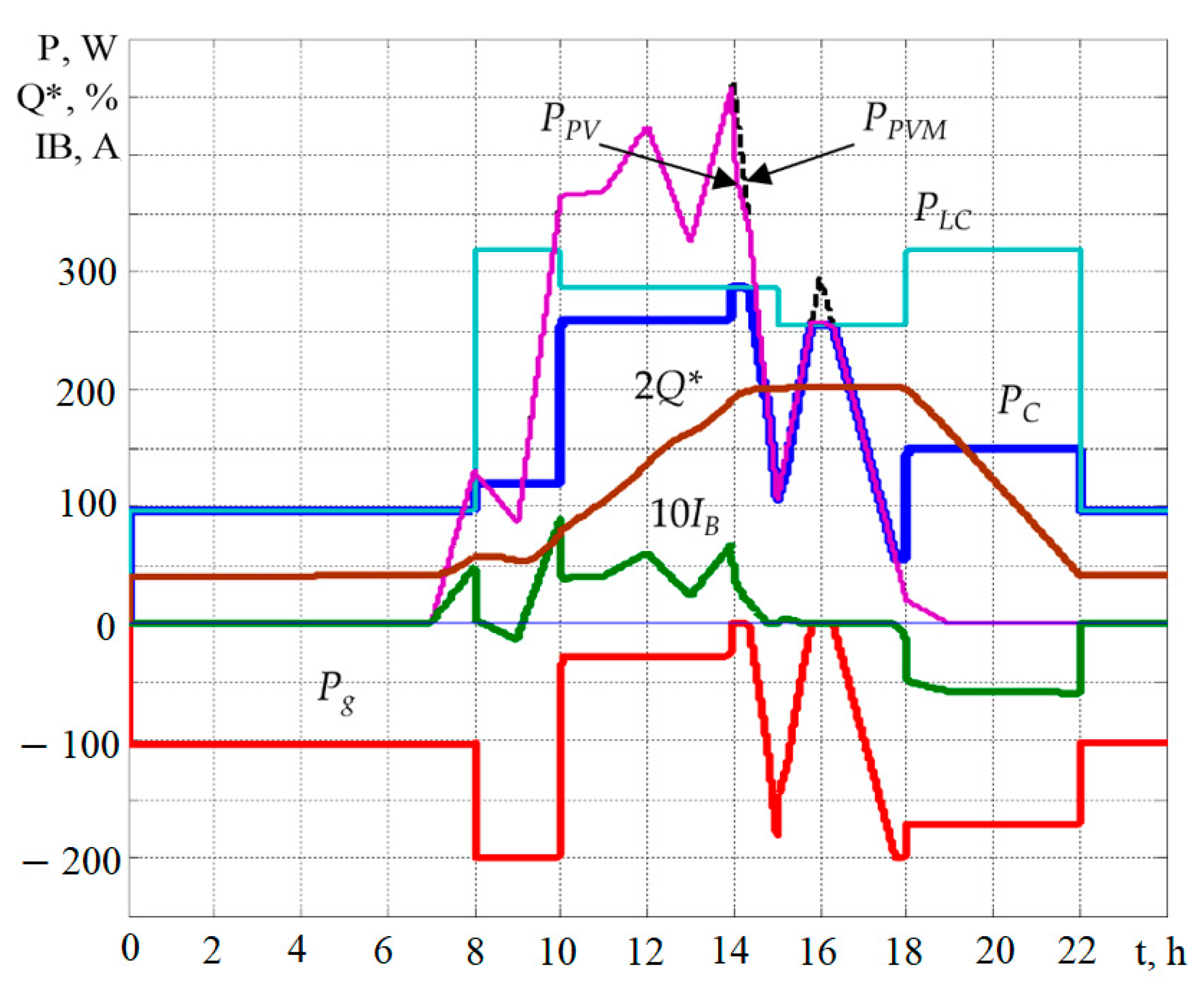
• In Figure 6 for the July day with a total generation in 3.3 times below the average (W_PV = 1320 Wh). In this case, k_E = 1.22, p = 1.6 (P_PVR = 0.86 kW, W_B = 800 Wh);
• In Figure 7a for the May day with the generation, corresponding to the average monthly values at P_LC = P_LCR, P_PVR = 1 kW, W_B = 968 Wh, and at limit values ρ = 1.95 with k_E = 2.618;
• In Figure 7b for the May day with the generation, corresponding to the average monthly values at P_LC = P_LCR, P_PVR = 0.86 kW, W_B = 800 Wh, and at limit values p = 1.8 with k_E = 2.356;
• In Figure 7c for the May day with the generation, corresponding to the average monthly values at P_LC≠P_LCR, P_PVR = 0.86 kW, W_B = 800 Wh, and p = 1.6 with k_E = 2.795;
• In Figure 8 for the September day with the generation, corresponding to the average monthly values at P_LC = P_LCR, P_PVR = 0.86 kW, W_B = 800 Wh, and ρ = 1.6 with k_E = 2.

Changing the reference of the added power P_C23 in the interval (t₂, t₃) from a fixed calculated value to the value corresponding to the actual PV schedule in the spring–autumn period allows increasing k_E by 2–4% with the exclusion of SB discharge.

7. Discussion of the Results of the Study on Increasing the Power of the LO Using PVS with SB

Increasing the load power of the LO above the limit of power consumption from the grid while reducing the installed power of PV and SB and decreasing the cost of paying for electricity, consumed by the LO, from the DG is possible due to the following:

-

Use of the basic schedule of added power, tied to the PV generation. This reduces the energy required for its implementation. This allows increasing the degree of power increase while reducing the energy capacity of the SB;

-

Limiting the degree of power increase at an intermediate value with a decrease in the installed power of the PV and SB. This provides an improvement in the use of PV energy without increasing the cost of electricity, consumed from the grid;

-

Referencing the current value of the added load power and the SOC value of the battery at time intervals, taking into account the predicted and actual PV generation. Due to the change in certain time intervals of the added power reference from the calculated value to a value that repeats the law of the change in the PV generation power, this contributes to more complete use of the PV energy;

-

Exclusion of the SB charge at night with the average monthly PV generation in the spring–summer–autumn period helps to reduce electricity consumption from the grid. This excludes battery discharge during the hours of the morning load peak, which helps to reduce the number of battery discharge cycles and increase its service life.

This article is a development of previous studies [19,26], which considered increasing the efficiency of hybrid PVS with SB for the needs of local facilities. This was achieved by reducing the cost of electricity consumed from the grid when using the PV generation forecast. A common problem is the significant overestimation of the PV power in relation to the load power of the LO, which is necessary for use in conditions of low PV generation.

As a result, even with medium PV generation, there is a significant underutilization of PV energy with the need for regulation of PV generation. A feature of the proposed solutions is a change in the general approach to the use of PV and SB energy when the load power, added to the limit, is formed. Directed formation of the graph of added power allows reducing the installed power of PV and SB.

There are certain limitations regarding the use of the results of the work, as described below.

-

An object was considered with the main load in the daytime in the presence of peak loads in the morning and evening hours. At the same time, it is possible to charge the SB at night within the limit on consumption from the grid;

-

The possibilities of increasing power are seasonal in nature with a maximum value in the period spring–summer–autumn;

-

The optimal choice of values for the degree of increase in power (ρ) and the installed PV power (m_P) involves taking into account many factors, including the costs of acquisition and ongoing maintenance. Such a task was not set in this work, and the approach was simplified for evaluation;

-

The assessment of a possible reduction in the cost of paying for electricity during the year was somewhat simplified and was performed for one tariff rate. We considered the days when the PV generation corresponds to the average monthly values for the accepted time intervals;

-

The implementation of the control system assumes an “open” structure of the relevant channels of control;

-

When modeling, it was assumed that the graph of the power generated by the PV corresponds to the forecast and does not change during the day.

Further development of this work is connected with the optimization of system parameters. It is also required to study the possibilities of correction of deviations in the values of the actual PV generation according to the forecast data and possible changes in the current forecast during the day.

8. Conclusions

With the selected parameters of the PVS, it is possible to increase the power of the LO over the limit for consumption from the grid up to 1.7–1.95 times. This depends on the average monthly PV generation of during the year. Limiting the degree of power increase to a value of 1.6, when choosing the parameters, allows reducing the installed power of the PV and SB. The possibility of increasing the degree of power increase to a value of 1.8 (if necessary) remains in this case.

It is advisable to select the parameters of the PVS on the basis of the data on the average monthly PV generation for the taken schedule of the load. It is possible to use archival data from web resources with open access at any point location of the object. The ratio of PV power and added load power is determined on the basis of PV generation in the transitional seasons (in this case, March and October). The energy capacity of the SB is determined by the power of the added load from the condition of the sufficiency of its operation in the pre-evening hours and evening peak hours with a given limitation of the DOD battery. The use of the basic schedule of the added power with reference to solar activity, while maintaining the resulting power of the LO, makes it possible to reduce the energy capacity of the SB. Therefore, when setting the degree of power increase ρ = 1.7 for winter, the energy capacity can be reduced by 13.5%. Limiting the value of ρ at the level of ρ = 1.6 allows reducing the installed power of the PV and the SB. When converted to the same total load power, the reduction for P_PVR is 9.4%, and that for W_BR is 14%.

The principle for controlling the power consumed by the LO from the grid in accordance with the reference value of the added load power and the total load power of the LO was developed. The reference of the value of the added power can be determined from the condition for the formation of the SOC(t) graph of the SB according to the PV generation forecast data.

At the same time, at certain time intervals, reference of the value of the added power can be carried out according to the schedule of the PV generation. This contributes to the maximum use of its energy. With the average monthly PV generation in the spring–autumn period, the SB discharge during the hours of the morning load peak is not used. Accordingly, the nighttime SB charge from the grid is not used. This helps to reduce consumption from the grid and reduce the number of deep discharge cycles, which contributes to longer battery life.

On the basis of a formalized description of energy processes in steady-state conditions for the daily cycle of the system’s functioning, the simulation of the system was completed. The simulation results showed that choosing the PVS parameters on the basis of ρ = 1.7 by setting ρ = 1.7–1.95 depending on the average monthly PV generation reduced the cost of electricity, consumed from the grid, for one rate of payment by 1.1 to 2.68 times. When choosing the PVS parameters on the basis of ρ = 1.6 and a constant degree of power increase during the year, it is possible to reduce electricity costs by up to 7% in the summer.

References

1. Rao, B.H.; Selvan, M.P. Prosumer Participation in a Transactive Energy Marketplace: A Game-Theoretic Approach. In Proceedings of the IEEE International Power and Renewable Energy Conference, Karunagappally, India, 30 October–1 November 2020. [Google Scholar]
2. Khezri, R.; Mahmoudi, A.; Aki, H. Optimal planning of solar photovoltaic and battery storage systems for grid-connected residential sector: Review, challenges and new perspectives. Renew. Sustain. Energy Rev. 2022, 153, 111763. [Google Scholar] [CrossRef]
3. ABB Solar Inverters. Product Manual REACT-3.6/4.6-TL (from 3.6 to 4.6 kW). Available online: https://www.abb.com/solarinverters (accessed on 9 March 2022).
4. Conext, S.W. Hybrid Inverter. Available online: https://www.se.com/ww/en/product-range-presentation/61645-conext-sw/ (accessed on 9 March 2022).
5. Zeng, Z.; Yang, H.; Zhao, R.; Cheng, C. Topologies and control strategies of multi-functional grid-connected inverters for power quality enhancement: A comprehensive review. Renew. Sustain. Energy Rev. 2013, 24, 223–270. [Google Scholar] [CrossRef]
6. Ma, T.-T. Power quality enhancement in micro-grids using multifunctional DG inverters. Lect. Notes Eng. Comput. Sci. 2012, 2196, 996–1001. [Google Scholar]
7. Shavelkin, A.; Jasim, J.M.J.; Shvedchykova, I. Improvement of the current control loop of the single-phase multifunctional grid-tied inverter of photovoltaic system. East.-Eur. J. Enterp. Technol. 2019, 6, 14–22. [Google Scholar] [CrossRef]
8. Belaidi, R.; Haddouche, A. A multi-function grid-connected PV system based on fuzzy logic controller for power quality improvement. Przeg. Elektr. 2017, 93, 118–122. [Google Scholar] [CrossRef] [Green Version]
9. Vigneysh, T.; Kumarappan, N. Grid interconnection of renewable energy sources using multifunctional grid-interactive converters: A fuzzy logic based approach. Electr. Power Syst. Res. 2017, 151, 359–368. [Google Scholar] [CrossRef]
10. Shavolkin, O.; Shvedchykova, I. Improvement of the Three-Phase Multifunctional Converter of the Photoelectric System with a Storage Battery for a Local Object with Connection to a Grid. In Proceedings of the 25th IEEE International Conference on Problems of Automated Electric Drive. Theory and Practice, PAEP 2020, Kremenchuk, Ukraine, 21–25 September 2020; pp. 1–6. [Google Scholar]
11. Shavolkin, O.; Shvedchykova, I.; Demishonkov, Y. Energy Management of Hybrid Three-Phase Photoelectric System with Storage Battery to Meet the Needs of Local Object. In Proceedings of the 20th IEEE International Conference on Modern Electrical and Energy Systems, MEES 2021, Kremenchuk, Ukraine, 21–24 September 2021. [Google Scholar]
12. Lliuyacc, R.; Mauricio, J.M.; Gomez-Exposito, A.; Savaghebi, M.; Guerrero, J.M. Grid-forming VSC control in four-wire systems with unbalanced nonlinear loads. Electr. Power Syst. Res. 2017, 152, 249–256. [Google Scholar] [CrossRef] [Green Version]
13. Guerrero-Martinez, M.A.; Milanes-Montero, M.I.; Barrero-Gonzalez, F.; Miñambres-Marcos, V.M.; Romero-Cadaval, E.; Gonzalez-Romera, E. A smart power electronic multiconverter for the residential sector. Sensors 2017, 17, 1217. [Google Scholar] [CrossRef] [Green Version]
14. Luthander, R.; Widén, J.; Nilsson, D.; Palm, J. Photovoltaic self-consumption in buildings: A review. Appl. Energy 2015, 142, 80–94. [Google Scholar] [CrossRef] [Green Version]
15. Yang, X.; Jiang, F.; Liu, H. Short-term power prediction of photovoltaic plant based on SVM with similar data and wavelet analysis. Prz. Elektrotech. 2013, 89, 81–85. [Google Scholar]
16. Mellit, A.; Pavan, A.M.; Lughi, V. Deep learning neural networks for short-term photovoltaic power forecasting. Renew. Energy 2021, 172, 276–288. [Google Scholar] [CrossRef]
17. Zsiborács, H.; Pintér, G.; Vincze, A.; Birkner, Z.; Baranyai, N.H. Grid balancing challenges illustrated by two European examples: Interactions of electric grids, photovoltaic power generation, energy storage and power generation forecasting. Energy Rep. 2021, 7, 3805–3818. [Google Scholar] [CrossRef]
18. Michaelson, D.; Mahmood, H.; Jiang, J. A Predictive Energy Management System Using Pre-Emptive Load Shedding for Islanded Photovoltaic Microgrids. IEEE Trans. Ind. Electron. 2017, 64, 5440–5448. [Google Scholar] [CrossRef]
19. Shavolkin, O.; Shvedchykova, I.; Jasim, J.M.J. Improved control of energy consumption by a photovoltaic system equipped with a storage device to meet the needs of a local facility. East.-Eur. J. Enterp. Technol. 2021, 2, 6–15. [Google Scholar] [CrossRef]
20. Forecast. Solar. Available online: https://forecast.solar/ (accessed on 9 March 2022).
21. Iyengar, S.; Sharma, N.; Irwin, D.; Shenoy, P.; Ramamritham, K. SolarCast—An open web service for predicting solar power generation in smart homes. In Proceedings of the 1st ACM Conference on Embedded Systems for Energy-Efficient Buildings, BuildSys 2014, Memphis, TN, USA, 3–6 November 2014; pp. 174–175. [Google Scholar]
22. Nicolson, M.L.; Fell, M.J.; Huebner, G.M. Consumer demand for time of use electricity tariffs: A systematized review of the empirical evidence. Renew. Sustain. Energy Rev. 2018, 97, 276–289. [Google Scholar] [CrossRef]
23. Davis, M.J.M.; Hiralal, P. Batteries as a Service: A New Look at Electricity Peak Demand Management for Houses in the UK. Procedia Eng. 2016, 145, 1448–1455. [Google Scholar] [CrossRef]
24. Lorenzi, G.; Silva, C.A.S. Comparing demand response and battery storage to optimize self-consumption in PV systems. Appl. Energy 2016, 180, 524–535. [Google Scholar] [CrossRef]
25. Badawy, M.O.; Cingoz, F.; Sozer, Y. Battery storage sizing for a grid tied PV system based on operating cost minimization. In Proceedings of the 2016 IEEE Energy Conversion Congress and Exposition, Milwaukee, WI, USA, 18–22 September 2016. [Google Scholar]
26. Shavelkin, A.A.; Gerlici, J.; Shvedchykova, I.O.; Kravchenko, K.; Kruhliak, H.V. Management of power consumption in a photovoltaic system with a storage battery connected to the network with multi-zone electricity pricing to supply the local facility own needs. Electr. Eng. Electromech. 2021, 2, 36–42. [Google Scholar] [CrossRef]
27. Shavolkin, O.; Shvedchykova, I.; Demishonkova, S.; Pavlenko, V. Increasing the efficiency of hybrid photoelectric system equipped with a storage battery to meet the needs of local object with generation of electricity into grid. Przeg. Elektr. 2021, 97, 144–149. [Google Scholar] [CrossRef]
28. Traore, A.; Taylor, A.; Zohdy, M.; Peng, F. Modeling and Simulation of a Hybrid Energy Storage System for Residential Grid-Tied Solar Microgrid Systems. J. Power Energy Eng. 2017, 5, 28–39. [Google Scholar] [CrossRef] [Green Version]
29. Miñambres-Marcos, V.M.; Guerrero-Martínez, M.Á.; Barrero-González, F.; Milanés-Montero, M.I. A grid connected photovoltaic inverter with battery-supercapacitor hybrid energy storage. Sensors 2017, 17, 1856. [Google Scholar] [CrossRef] [PubMed] [Green Version]
30. Photovoltaic Geographical Information System. Available online: https://re.jrc.ec.europa.eu/pvg_tools/en/tools.html#SA (accessed on 9 March 2022).
31. Data Sheet. Lithium Iron Phosphate (LiFePo4) Battery 12.8 V 150 Ah. Available online: https://www.enix-energies.com (accessed on 9 March 2022).
Figure 1. Simplified structure of power supply of LO load.
Energies 15 04883 g001
Figure 2. Structure of hybrid PVS with SB.
Energies 15 04883 g002
Figure 3. Formation of schedule of state of the charge of SB.
Energies 15 04883 g003
Figure 4. Structure of the control system of PVS.
Energies 15 04883 g004
Figure 5. Oscillograms PLC, PC, PPV, Q , IB, and Pg for a December day with general generation WPV = 500 Wh ( Q and IB values are shown at scale 2 and 10, respectively).
Energies 15 04883 g005
Figure 6. Oscillograms PLC, PC, PPV, Q , IB, and Pg for a July day with general generation WPV = 1320 Wh ( Q and IB values are shown at scale 2 and 10, respectively).
Energies 15 04883 g006
Figure 7. Oscillograms PLC, PLCR, PC, PPVM, PPV, Q , IB, and Pg for the May day with a generation corresponding to the monthly average ( Q and IB values are shown at scale 2 and 10, respectively): (a) PLC = PLCR, PPVR = 1 kW, WB = 968 Wh, and at limit values ρ = 1.95 with kE = 2.618; (b) PLC = PLCR, PPVR = 0.86 kW, WB = 800 Wh, and at limit values p = 1.8 with kE = 2.356; (c) PLCPLCR, PPVR = 0.86 kW, WB = 800 Wh, and p = 1.6 with kE = 2.795.
Energies 15 04883 g007aEnergies 15 04883 g007b
Figure 8. Oscillograms PLC, PLCR, PC, PPVM, PPV, Q , IB, and Pg for the September day with the generation, corresponding to the average monthly values at PLC = PLCR, PPVR = 0.86 kW, WB = 800 Wh, and ρ = 1.6 with kE = 2 ( Q and IB values are shown at scale 2 and 10, respectively).
Energies 15 04883 g008