Abstract
Wind power utilization is attracting worldwide attention in the renewable energy field, and as wind power develops from land to sea, the size of the blades is becoming incredibly larger. The fatigue test, especially the biaxial synchronous fatigue test for the blades, is becoming an indispensable step to ensure the blade’s quality before mass production, which means the biaxial independent test presently used may have difficulty reproducing the real damage for large-sized blades that oscillate simultaneously in flap-wise and edgewise directions in service conditions. The main point of the fatigue test is to carry out accelerated and reinforced oscillations on blades in the experimental plan. The target moments of critical blade sections are reached or not during the test are treated as one significant evaluation criterion. For independent tests, it is not hard to realize moment matching using additional masses fixed on certain critical blade sections, which may be not easy to put into effect for biaxial synchronous tests, since the mechanical properties and target moments in the flap-wise and edgewise directions are widely varied. To realize the mechanical decoupling for loading force or additional mass inertia force in two directions is becoming one of the key issues for blade biaxial synchronous fatigue testing. For this problem, the present paper proposed one mechanical decoupling design concept after a related literature review. After that, the blade moment design and target matching approach are also proposed, using the Transfer Matrix Method (TMM) for moment quick calculation and Particle Swarm Optimization (PSO) for case optimization.
1. Load Equivalence Mechanism for Fatigue Test of Wind Turbine Blades
Before a detailed comparison of the mechanical decoupling methods for the moment matching of the biaxial synchronous fatigue test, the fatigue test procedure and the biaxial loading moment-matching requirements are briefly introduced.
1.1. Acceleration Mechanism of the Fatigue Test
To reproduce the real conditions in the natural environment, the blade fatigue test would take such a long time that it is unacceptable. Natural loads are usually time-varying and random, so loading millions of times is impractical. So, before the fatigue testing of wind turbine blades, how to strengthen the natural load from random to equal amplitude and how to simplify the testing technology and shorten the testing period are the primary goals. As introduced, the primary works could be briefly summarized with five steps as follows:
- (1)
- Load calculation
Fatigue analysis is based on load spectrum, and load can be counted and calculated using different methods. On this basis, the load spectrum of the fatigue analysis can be determined, for example, by measurement or computer simulation [1,2,3]. The periodic loads of wind turbine blades mainly include pneumatic loads and mechanical loads, such as gravity and inertial forces. The actual load at a certain position of the blade can be measured by using sensors such as strain gauges [4]. This method often requires a long testing time and huge testing cost, which is in line with the actual situation. In addition, the aerodynamic load of a blade can be computed according to strip theory, through which the normal force and tangential force of the blade can be obtained. After that, the aerodynamic moment of a certain section is obtained, which varies with different wind speed segments [5].
- (2)
- Compilation of load spectrum
After calculating the load, the finite element simulation method is adopted, endowing the blade model with real material properties. At the same time, the aerodynamic load and mechanical load calculated above are applied to solve the stress–time history of a certain section of the blade, and then the rain flow counting method is used to obtain the relationship between stress and cycle times [6,7]. When investigating the accumulation of fatigue damage of blades, it is necessary to calculate the cycle times of the aerodynamic load at various wind speeds, while the Weibull distribution function can be used to describe the wind speed distribution, so as to obtain the annual cumulative hours of a certain wind speed section, then calculate the annual cycle times of corresponding stress [8,9,10,11].
- (3)
- Cumulative damage modeling
The fatigue model of materials generally uses the S–N curve, which can be expressed as [12,13,14,15,16,17]:
where are parameters related to material properties, style, stress ratio and loading mode. is the stress amplitude, and is the number of stress cycles before material failure.
According to Palmgren Miner’s linear cumulative damage theory, the damage can be regarded as a linear cumulative relationship with stress cycle. When the damage accumulates to a certain critical value, the damage will be produced as follows:
where is the Miner coefficient; when , the material is expected to fail. is the cycle number of load ; is the load cycle number when the material fails under the action of load .
- (4)
- Goodman correction
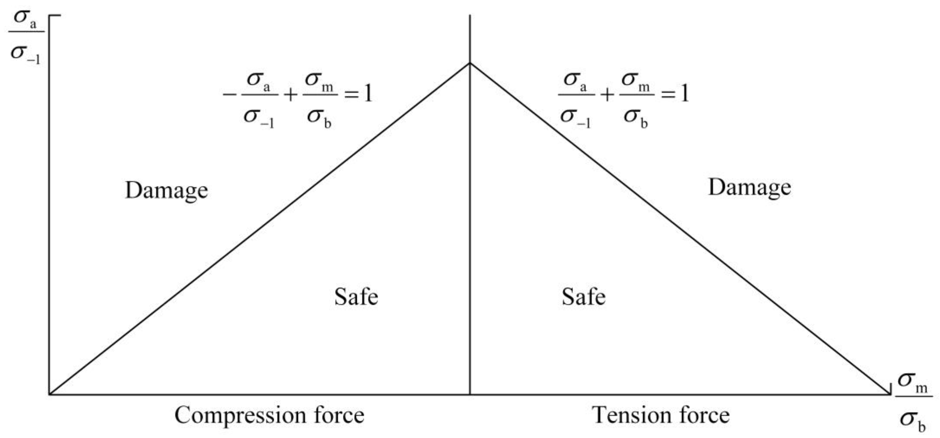
The S–N curve of the material is obtained under the specified stress ratio . Under the specified life cycle, the conditional fatigue limit under different stress ratios can be obtained according to the modified Goodman curve equation [18,19,20,21]. The Goodman curve is shown in Figure 1:
where is the stress amplitude, is the average stress, is the material static strength, and is the required conditional fatigue limit.

Figure 1.
Goodman Guidelines.
After the correction above, the symmetrical cyclic stress and the corresponding cycle times can be obtained and can be brought into the S–N curve to calculate the corresponding life cycle.
- (5)
- Determination of equivalent load
The equivalent load is determined using the following steps [22].
The cumulative damage amount determined by the load spectrum is:
The equivalent load cumulative damage is:
Setting and taking as the desired equivalent load loading times, the equivalent test load can be obtained, which is a constant amplitude symmetrical load.
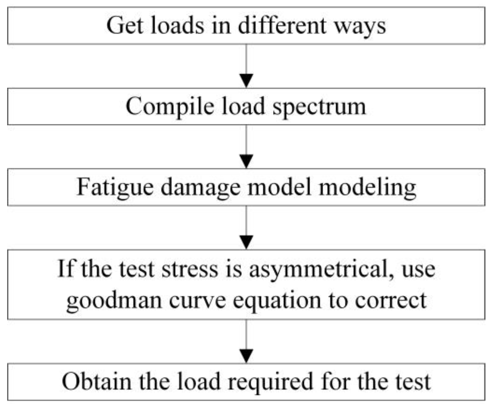
The above load calculation process can be summarized as shown in Figure 2.
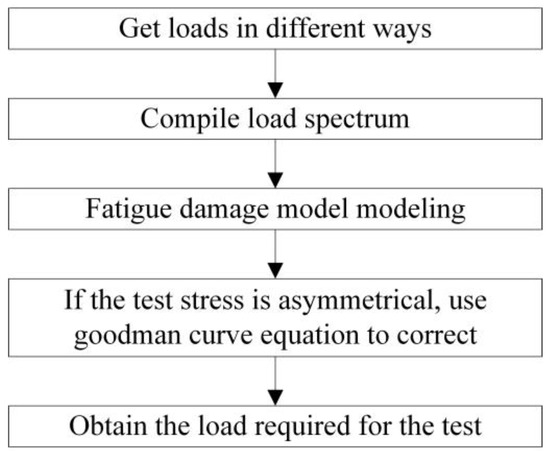
Figure 2.
Methods of accelerating fatigue test.
In some recent studies, aeroelastic simulations in the process of load analysis were considered [23,24,25].
1.2. Biaxial Loading and Its Bending Moment-Matching Requirements
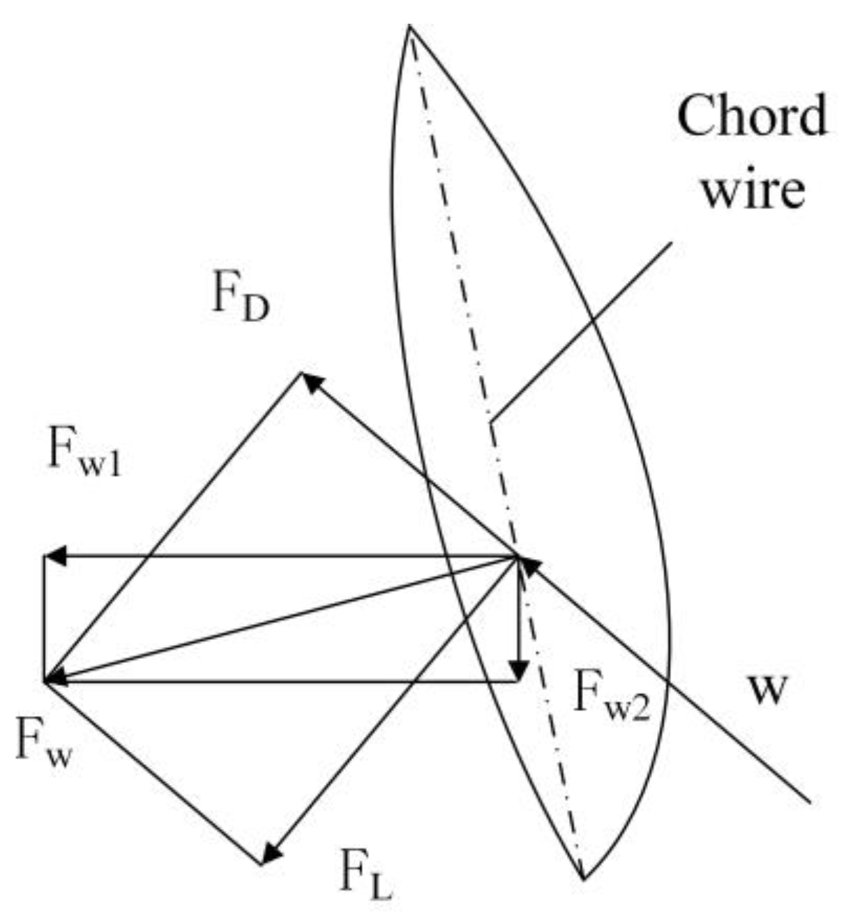
In order to generate a rotating moment to rotate the wind turbine blade, the chord line of the blade usually keeps a certain angle with the horizontal direction, as shown in Figure 3. While the wind turbine is running, the incoming wind effects on the blades to generate a wind pressure composed of lift and drag , while can be decomposed into flap-wise force and edgewise force . In the uniaxial fatigue test, the force decoupling device only applies force either flap-wise or edgewise to the blade, which is obviously not completely consistent with the actual force situation of the blade. In the actual use of blades, the fatigue damage is caused by the loads of both flap-wise and edgewise directions, so a biaxial synchronous test is more accurate than a biaxial independent or uniaxial test [26,27]. Compared with the biaxial independent test, the advantage of synchronous method is that, the test damage is caused by the resultant force of the two-direction load, the method of producing the damage is closer to the actual use process. Therefore, more accurate test results can be obtained. In addition, the synchronous biaxial loads are loaded and ended at the same time, so the test period is shortened by half, which greatly improves the test efficiency.
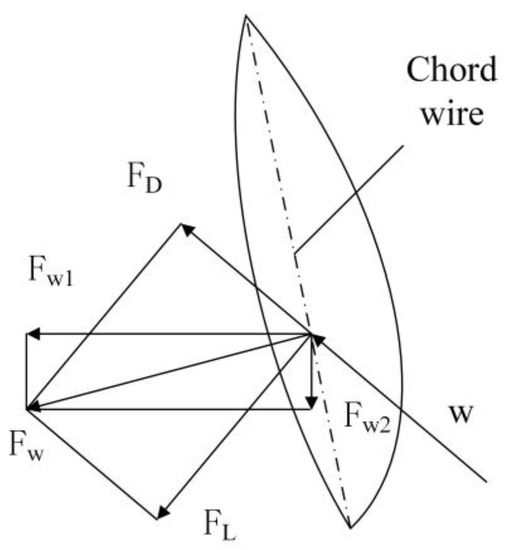
Figure 3.
Force diagram of blade section.
Loading approaches of wind turbine blades can be divided into forced displacement type and resonance type [28,29,30,31]. In the forced displacement loading mode, hydraulic loaders are generally used to drive the blades to move forcibly. In the resonant loading mode, certain masses are usually added to the blades to adjust bending moment distribution and natural frequency, while vibration exciters are used for loading.
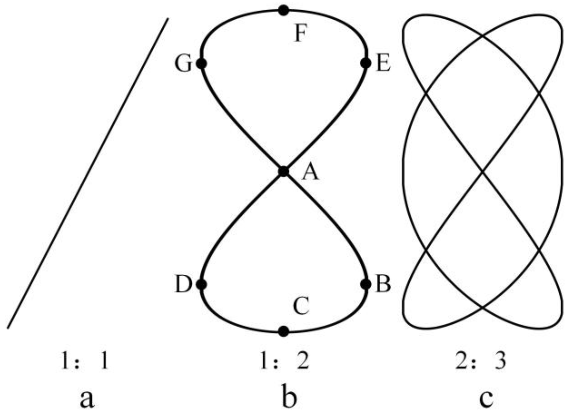
As shown in Figure 4, if the resonance loading test scheme is adopted, and the vibration exciter excites the blade resonance. There will be many options for the frequency ratio which means the ratio of flap-wise resonance frequency to edgewise resonance frequency. In addition, when the test frequency ratio is 1:1, the blade section trajectory can also be an ellipse [32]. Since the frequency ratio of a 50–60 m blade tends to be 1:2, the frequency ratio of this paper is determined to be 1:2. Under this condition, in a single cycle, the movement track of any point on any section of the blade can be shown in Figure 4b, while its position sequence track is A-B-C-D-A-E-F-G-A.

Figure 4.
Movement track of blades at different frequency ratios. (a–c) represent the motion trajectory of the point on the blade when the frequency ratio is 1:1, 1:2 and 1:3 respectively.
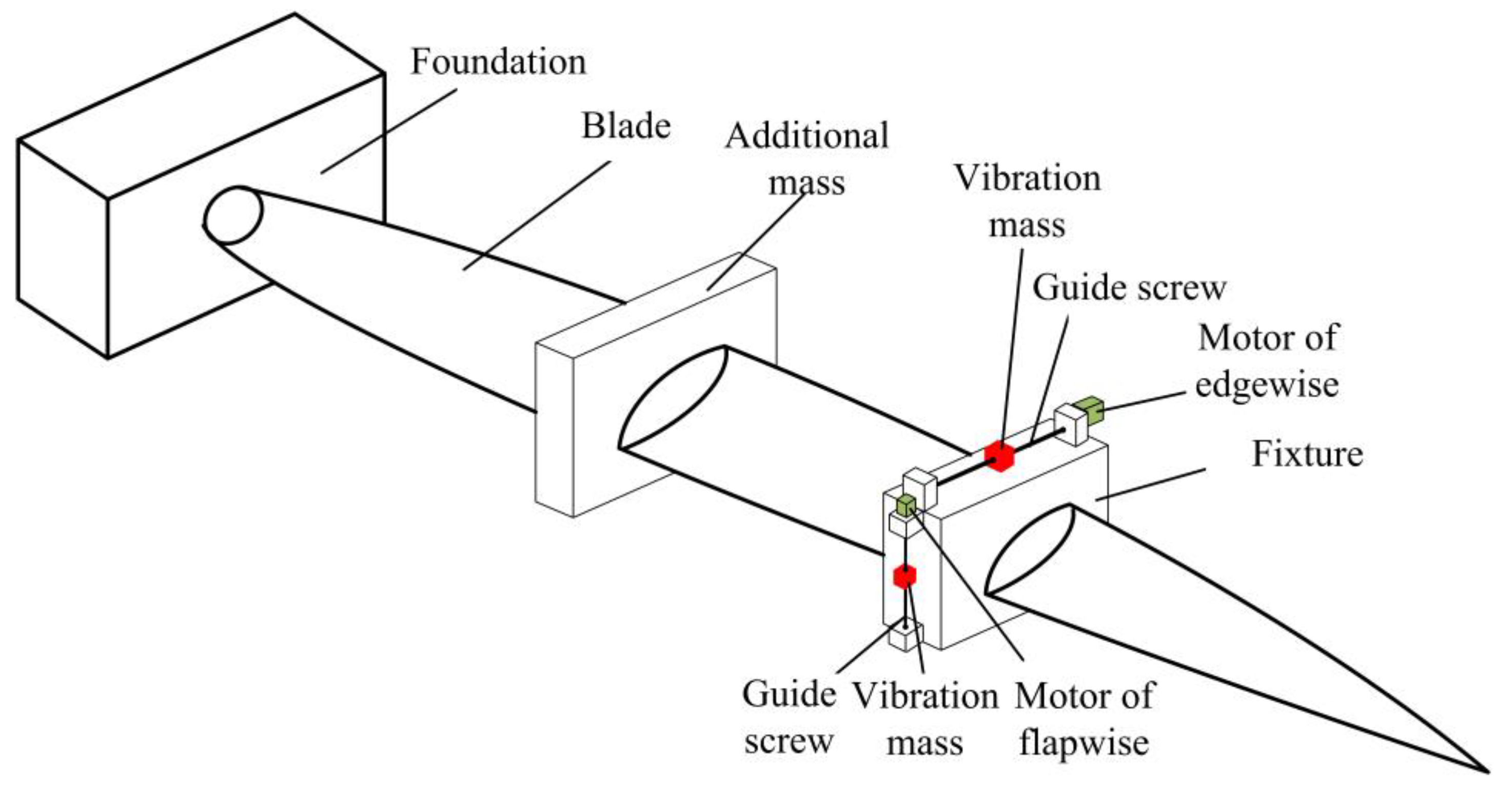
As shown in Figure 5, if the popular resonance loading method is adopted biaxially, it can be found from Figure 3 that in the biaxial resonance fatigue test, the mass block installed on the blade will change the bending moment distribution in both directions at the same time, so that the bending moments in the flap-wise and edgewise tests in the existing loading equipment cannot meet the target bending moment requirements at the same time. Therefore, it is necessary to design a new type of loading equipment to decouple the bending moment, so that the bending moments in both directions of the blade can meet the requirements at the same time.

Figure 5.
Biaxial resonant fatigue testing device.
2. Existing Biaxial Force Decoupling Devices and Their Error Analysis
2.1. Forced Displacement Biaxial Testing Device
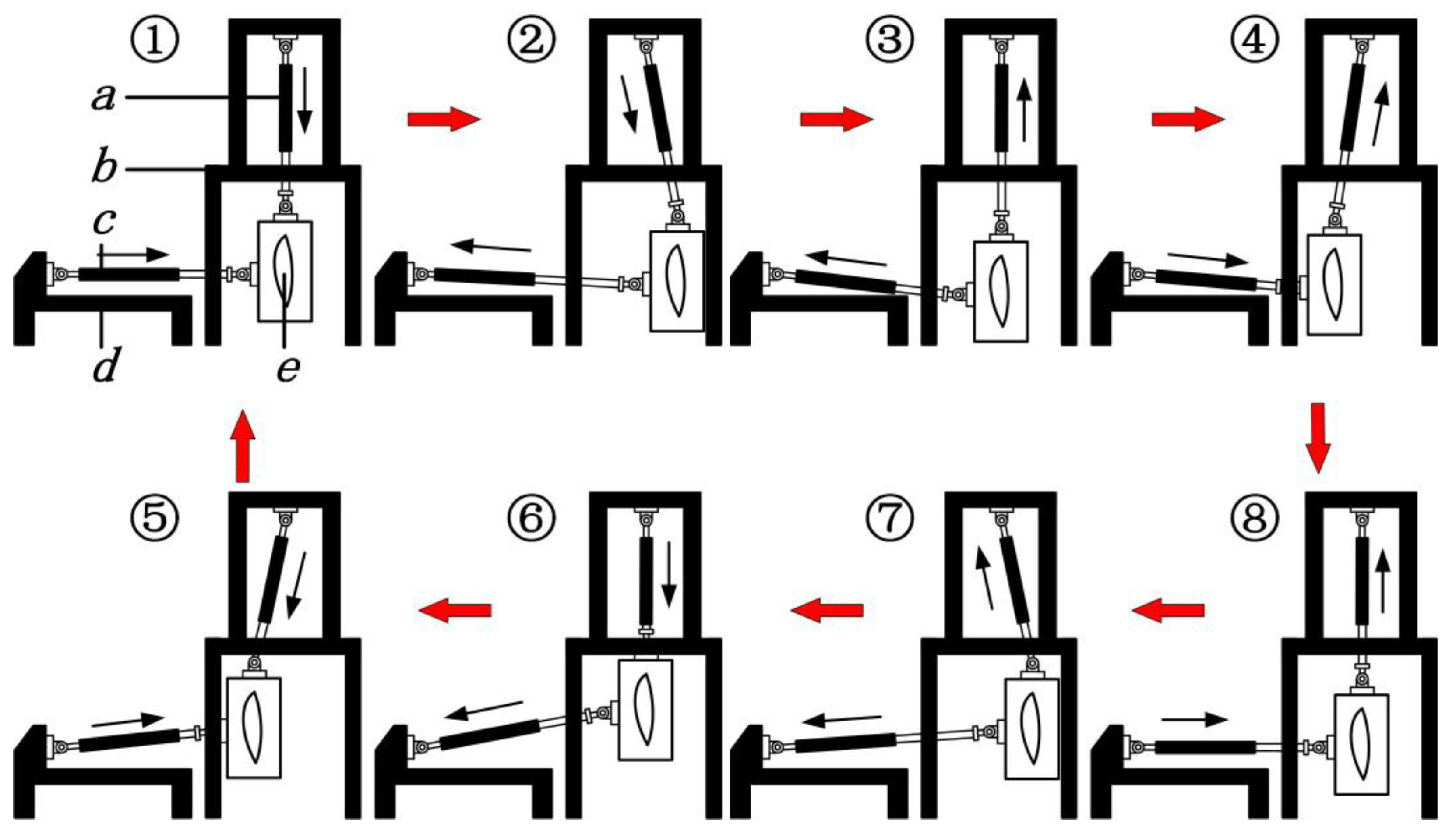
The world’s earliest biaxial fatigue testing device is forced displacement type, which was put forward by D.R.V.Van et al. of Delft University of Technology in the Netherlands in 1986 [28]. As shown in Figure 6, the force decoupling device consists of support frames, a flap-wise hydraulic loader, an edgewise hydraulic loader, a fixture, etc. Because the piston rod is fixedly connected with the blade through the fixture, the hydraulic loader forcibly drives the blade to reciprocate during the test. In one cycle, the direction change of the acting force of flap-wise hydraulic loader and edgewise hydraulic loader on the blade is shown in Figure 6. Under the constantly changing outside force, the blade position experiences the movement process of 1-2-3-4-5-6-7-8-1.
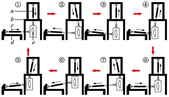
Figure 6.
Movement process of blades in a single cycle when using forced displacement biaxial testing device. a is hydraulic loader of edgewise, b is support frame, c is hydraulic loader of flapwise, d is support frame, e is cross section of blade and fixture.
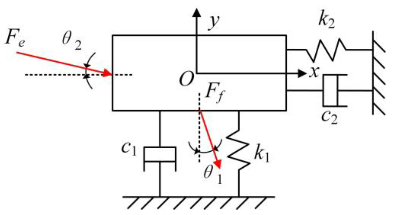
According to the equivalent principles of mass, damping, and stiffness in mechanical vibration [33,34], the equivalent model of blade testing system can be established as shown in Figure 7. According to dynamic analysis, the following equations can be deduced:
where is the force exerted on the blade by the flap-wise hydraulic loader, is the force exerted on the blade by the edgewise hydraulic loader of, is the angle between the flap-wise force and the vertical direction, is the angle between the edgewise force and the horizontal direction, and and are the displacements of the edgewise and flap-wise blades, respectively. and are the flap-wise and edgewise damping, respectively. and are the stiffnesses of the flap-wise and edgewise blades, respectively, and is the blade mass.

Figure 7.
Equivalent model of blade testing system forced displacement biaxial testing device.
The flap-wise exciting force , edgewise exciting force , angles and , damping and , and stiffnesses satisfy the following relationships, respectively:
where and are the amplitude of flap-wise force and edgewise force, respectively, is the flap-wise force loading frequency, is the edgewise force loading frequency, is the flap-wise natural frequency, is the edgewise natural frequency. and is damping ratio of flap-wise and edgewise, respectively. and is the Maximum amplitude at blade excitation point of flap-wise and flap-wise, respectively. are push rod length of hydraulic loader’s length of flap-wise and edgewise, respectively.
According to Equations (6) and (7), there are:
where and are the resultant forces of the flap-wise and edgewise blades, respectively.
According to Equation (9), the resultant force in the flap-wise (edgewise) direction of the blade is composed of the vertical (horizontal) component of flap-wise loading force and the vertical (horizontal) component of edgewise loading force . Therefore, the actual loads of the flap-wise and edgewise blades in the test process do not meet the test requirements, which affects the test results.
In addition, because the forced displacement loading mode is adopted in both directions during the test, the device may cost a lot of energy [35]. In order to reduce the energy loss in the test process and reduce the coupling of loading force to a certain extent, a resonance test method has been applied to the blade fatigue test.
2.2. Hybrid Biaxial Testing Device
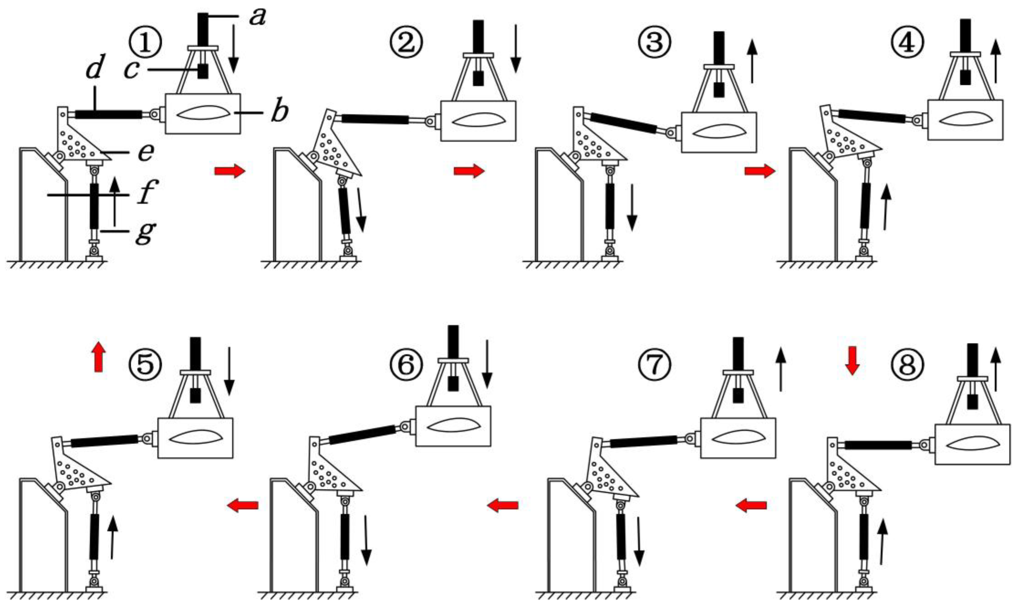
In 2004, NREL [36] proposed a hybrid test device as shown in Figure 8, which consists of flap-wise hydraulic loader, edgewise hydraulic loader, exciting mass, support frame, rocker arm, and push rod, etc. In the test, the flap-wise hydraulic loader drives the exciting mass block to reciprocate up and down, the motion frequency is close to the flap-wise natural frequency of the blade to excite the blade resonating in flap-wise. Force drives the blade to reciprocate in the horizontal direction by edgewise hydraulic loader. In a single cycle, the direction change loop of the force exerted by the flap-wise hydraulic loader and the edgewise hydraulic loader is shown in Figure 8. Under the action of a constantly changing external force, the position of the blade has experienced 1-2-3-4-5-6-7-8-1 movement.

Figure 8.
Movement process of blades in a single cycle when using hybrid biaxial fatigue testing device. a is hydraulic loader of flapwise, b is cross section of blade and fixture, c is hydraulic rod and vibration mass, d is push rod, d is push rod, e is rocker arm, f is foundation, g is hydraulic loader of edgewise.
According to the equivalent principles of mass, damping, and stiffness in mechanical vibration [33,35], the equivalent model of blade testing system can be established as shown in Figure 9. According to the dynamic analysis, it can be deduced that:
where is the force exerted on the blade by the flap-wise hydraulic loader, is the force exerted on the blade by the edgewise hydraulic loader, is the angle between the flap-wise force and the vertical direction, is the angle between the edgewise force and the horizontal direction, and are the displacements of the edgewise and flap-wise blades, respectively. and are the damping of the flap-wise and edgewise blades, respectively. and are the stiffnesses of the flap-wise and edgewise, respectively, and is the blade mass.
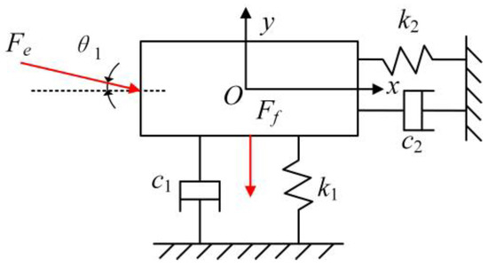
Figure 9.
Equivalent model of hybrid biaxial fatigue testing device.
The flap-wise exciting force , edgewise exciting force , angle , damping , and stiffnesses satisfy the following relationships, respectively:
where and are the amplitudes of the flap-wise force and the edgewise force, respectively, is the flap-wise force loading frequency, is the edgewise force loading frequency, is the flap-wise natural frequency, and is the edgewise natural frequency. and are the maximum amplitudes at the flap-wise and edgewise blade excitation point, respectively. are the push rod lengths of the flap-wise and edge-wise hydraulic loader’s length, respectively.
Substitute Equations (11) into Equation (10):
where and are the resultant flap-wise and edgewise forces, respectively.
According to Equation (13), the resultant flap-wise force is composed of the vertical components of the flap-wise loading force and the edgewise loading force , and the resultant force of the edgewise is the horizontal component of the edgewise loading force . So, the test bending moment of the flap-wise force is determined by and , which means that the force exerted on the blade by the edgewise hydraulic loader will affect the bending moment distribution in both directions at the same time, so that the bending moment error in both directions on the blade may not meet the bending moment requirements.
In addition, because the resonant loading mode has lower energy consumption than the forced displacement loading mode, the flap-wise force adopts the mixed biaxial fatigue test of the resonant loading mode, which would generally reduce the energy consumption by about 65% compared with the forced displacement fatigue test [35]. However, edgewise in the hybrid biaxial fatigue test adopts the forced displacement loading mode, the energy consumption is still high, so the device does not meet the requirement of low energy consumption in the fatigue tests of large blades.
2.3. “Virtual Mass” Biaxial Testing Device
In 2016, the NREL [36] schemed out the “Virtual Mass” biaxial testing device, which is composed of a hydraulic loader, a push rod, a fixture and virtual-mass, etc. In 2020, Melcher, D. et al. [37] designed a new elliptical biaxial resonance test method using virtual mass.
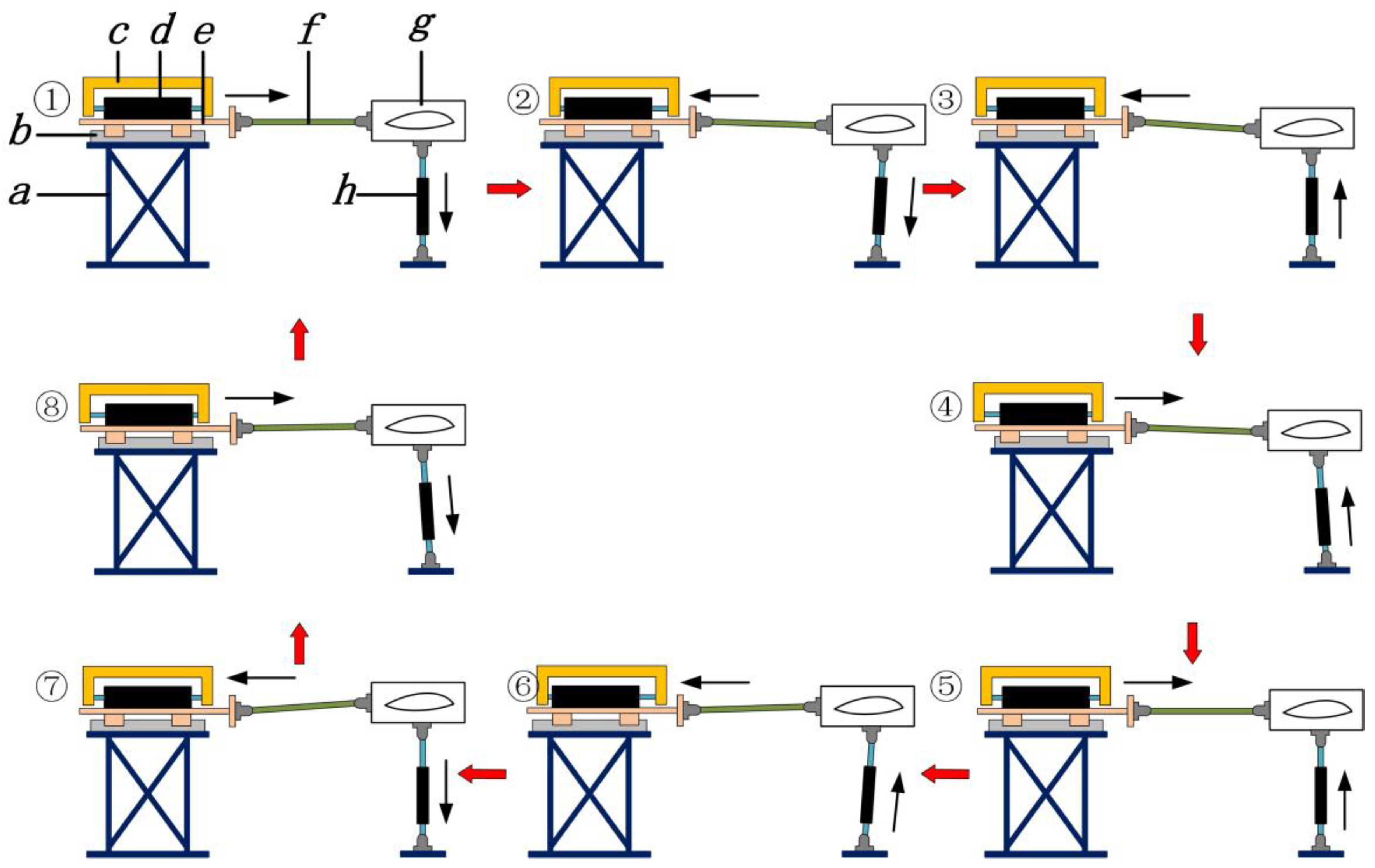
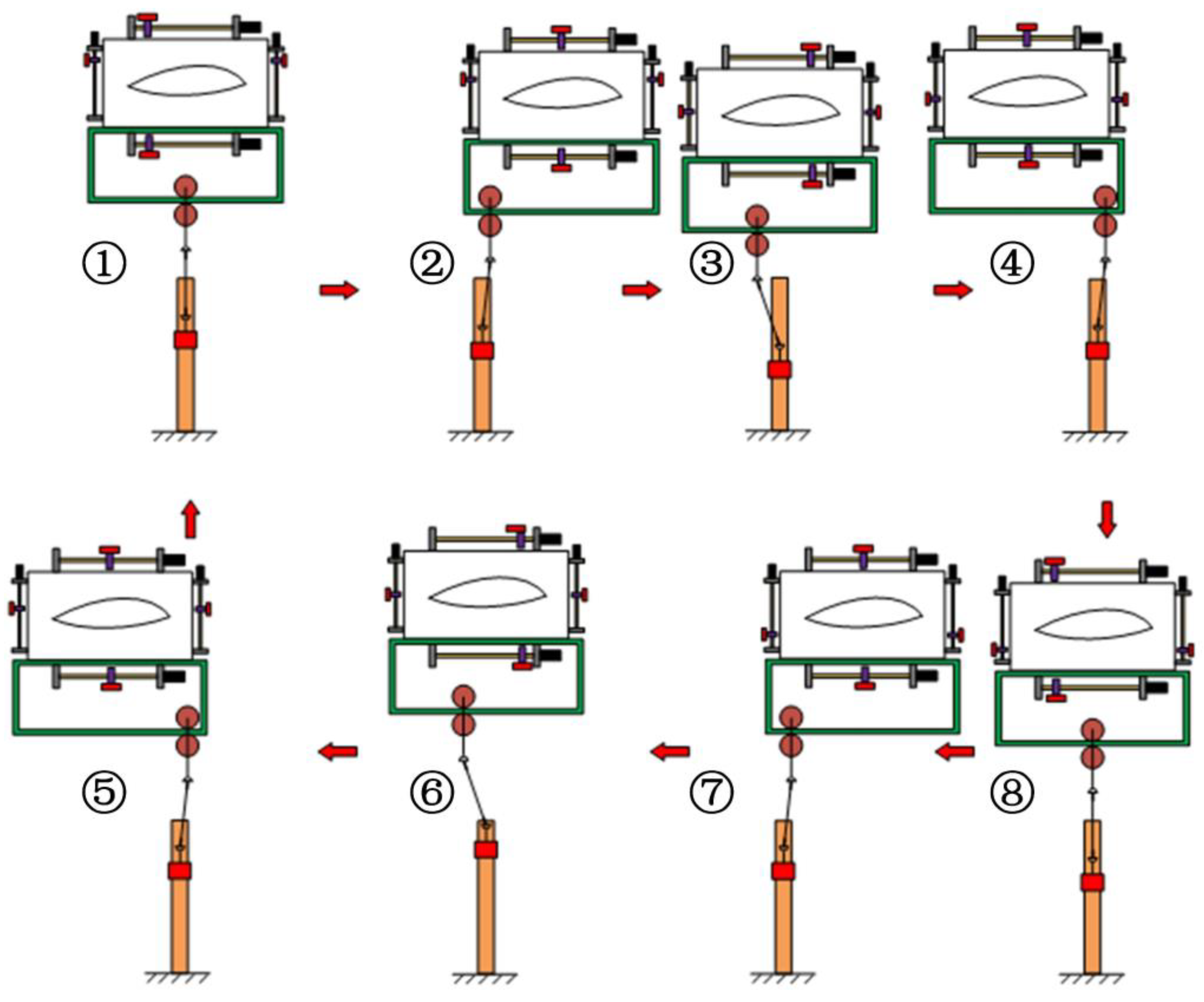
The device is shown in Figure 10. In the test, a flap-wise hydraulic loader drives the blade to reciprocate up and down at a certain frequency. The edgewise hydraulic loader applies an exciting force with a frequency similar to the natural frequency of the blade to excite the resonance of the blade through the virtual-mass in the horizontal reciprocating motion. The acting force direction of flap-wise hydraulic loader and edgewise hydraulic loader on the blade in a single-cycle changes are shown in Figure 10. Under the action of a constantly changing outside force, the position loop of the blade goes through 1-2-3-4-5-6-7-8-1. The concept of virtual-mass means that the mass block is indirectly connected with the blade through a push rod and a fixture, while only the bending moment distribution in one direction of the blade is adjusted.
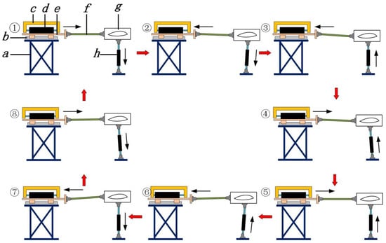
Figure 10.
Movement process of blades in a single cycle when using “virtual-mass” biaxial fatigue testing device. a is foundation, b is slide rail, c is virtual mass, d is hydraulic loader of edgewise and piston rod, e is slide platform, f is push rod, g is cross section of blade and fixture, h is hydraulic loader of flapwise.
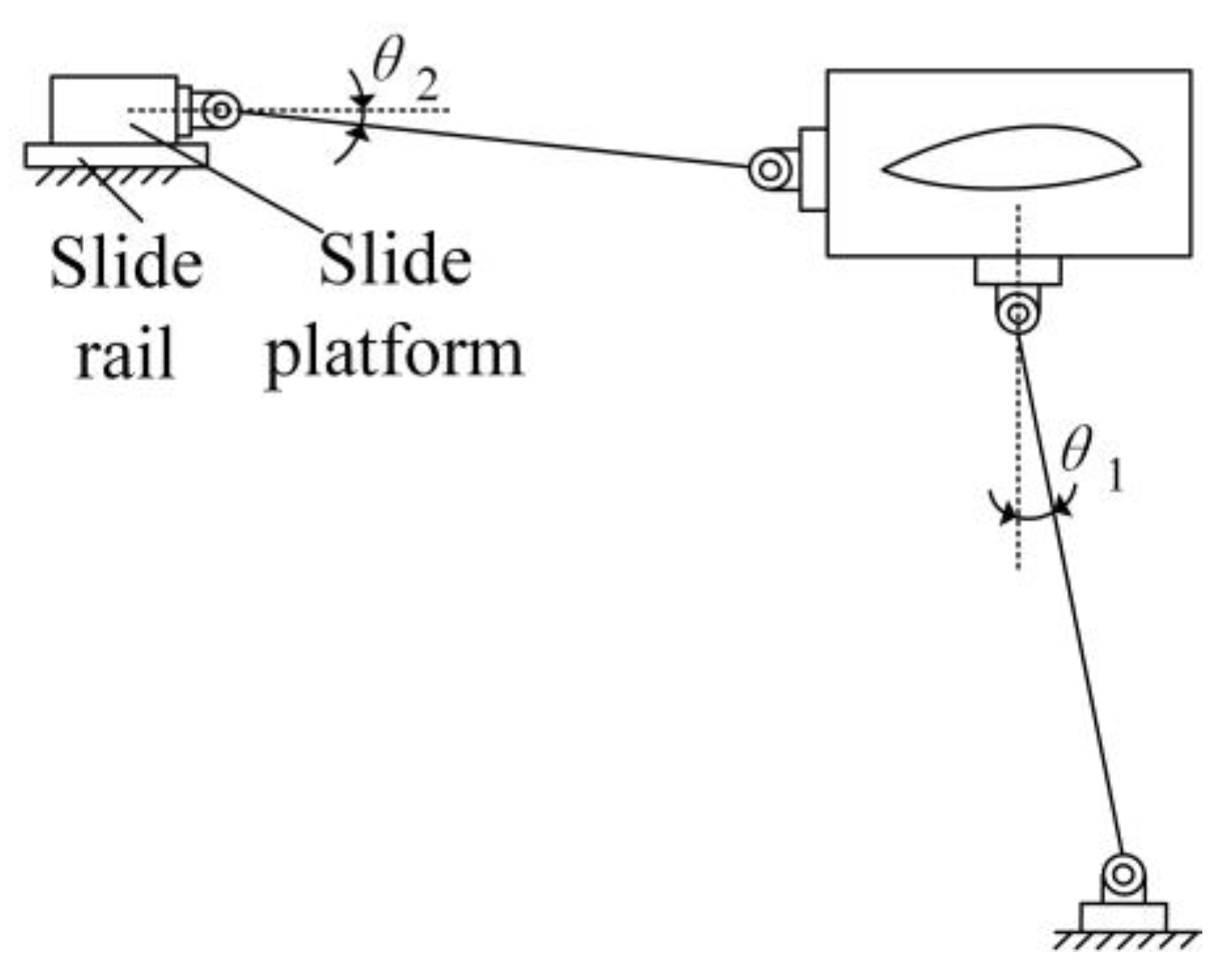
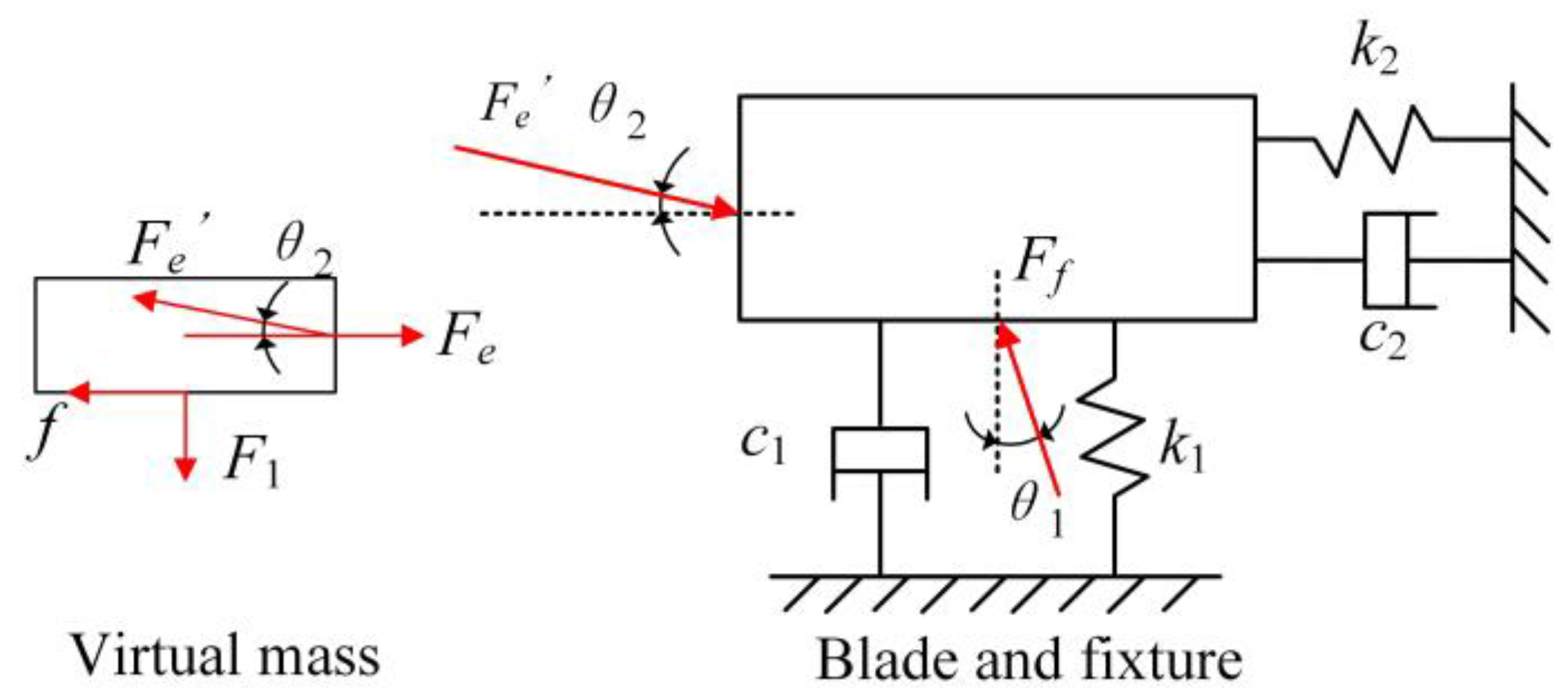
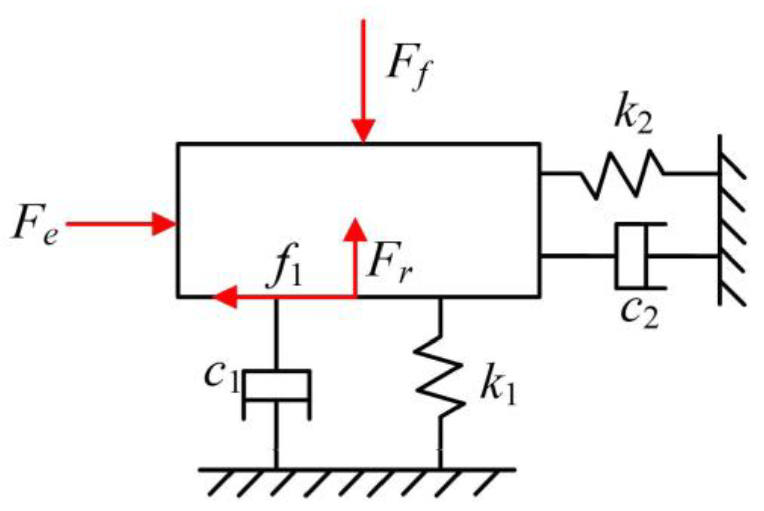
According to the equivalent principles of mass, damping, and stiffness in mechanical vibration [33,35], the equivalent model of a blade testing system can be established as shown in Figure 11 and Figure 12 Here, the virtual mass block, edgewise hydraulic loader, and sliding platform are simplified as sliding devices. According to the force analysis, it can be deduced that:
where is the force exerted on the blade by the flap-wise hydraulic loader, is the force exerted on the blade by the edgewise hydraulic loader, is the force exerted by the push rod on the sliding device, is the friction force between the sliding device and the slide rail, is the supporting force of the slide rail on the sliding device, is the angle between the flap-wise force and the vertical direction, is the angle between the edgewise force and the horizontal direction, and and are the displacements of the edgewise and flap-wise blades, respectively. and are the flap-wise and edgewise damping, respectively. and are the stiffnesses of flap-wise and edgewise blades, respectively. is the mass of the slide device, and is the blade mass with the fixture.

Figure 11.
Schematic diagram of test structure.
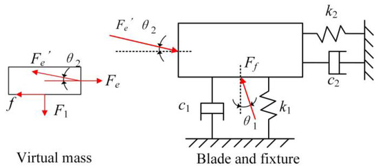
Figure 12.
Force diagram of structure.
The flap-wise exciting force , edgewise exciting force , angles and , damping and , and stiffness satisfy the following relationships:
where and are the amplitudes of the flap-wise force and edgewise force, respectively, is the flap-wise force loading frequency, is the edgewise force loading frequency, is the flap-wise natural frequency, and is the edgewise natural frequency. is the coefficient of the sliding friction between rail bearing and the rail. are the flap-wise and edgewise damping ratios, respectively. are the maximum amplitudes at the flap-wise and edgewise blade excitation points, respectively. are push rod lengths of the flap-wise and edgewise hydraulic loader’s lengths, respectively.
According to Equations (14) and (15), and considering the negligible friction, there are:
where and are the resultant forces in theflap-wise and edgewise directions. and satisfy the following relationship:
Compared with the biaxial forced displacement loading and hybrid biaxial testing, the virtual-mass loading device adopts resonant loading in both directions, which has lower energy consumption. However, Equation (17) shows that the force exerted on the blade by the flap-wise and edgewise hydraulic loaders will affect the bending moment distribution in both directions at the same time, leading the moment matching to result in errors.
Assuming that the virtual-mass is installed flap-wise, since the virtual-mass’s cross section is farthest from the blade root, the change in the push rod angle has the most obvious influence on the bending moment of the blade root. Thus, the blade root section is taken as an example to calculate. Compared with the push rod not deflecting, the calculation equation of the bending moment error caused by the deflection angle when the deflection angle of the push rod is maximum is as follows:
where is the bending moment generated by virtual-mass only in the flap-wise direction when the push rod is not deflected, and are the bending moments generated by the total mass of the blade and the mass block on the blade in the flap-wise and edgewise directions, respectively, when the push rod is not deflected. When the blade is at the extreme position, is the maximum deflection angle of the push rod, is the flap-wise moment error at the limit position, and is the edgewise moment error at the limit position.
The maximum deflection angle can be calculated as follows:
where is the amplitude of blade in edgewise at the virtual-mass installation position, and is the length of the push rod.
Take a 60 m-long blade as an example to calculate. , , , and of the edgewise blade are 1.08 m, 518.5 kN·m, 3852 kN·m, and 5250 kN·m, respectively. Because the amplitude of the flap-wise blade is 3.69 m, the rod length must be greater than 3.69 m to prevent the blade from colliding with the guide rail. According to the above data, the variation trend of the bending moment error in both directions at the limit position with the increase in rod length is shown in Figure 13.
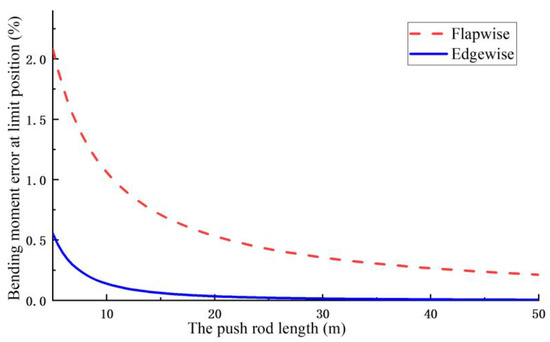
Figure 13.
Change trend diagram of bending moment error with the increase in rod length.
As shown in Figure 13, assuming that the rod length is 5 m, it can be known from calculation that the bending moment error at the limit position exceeds 2%. In order to reduce the error, it is necessary to increase the rod length. However, increasing the rod length will affect the stability of the mechanism, and the additional mass of the rod will also affect the loading accuracy. What is more, in order to reduce the influence of the rod itself on the error, the testing device requires the material of the rod to be as rigid and light as possible. Materials meeting this requirement usually cannot bear excessive shear force and are prone to fatigue failure, which may fail before the end of the test.
3. A Newly Designed Biaxial Synchronous Force Decoupling Device and Its Mechanism, Error, and Advantages Analysis
3.1. Structural Design of the New Force Decoupling Device
In order to solve the problem of loading force coupling in the virtual mass type loading device, the authors proposed one biaxial force decoupling design as shown in Figure 14 which is mainly composed of a flap-wise vibration exciter, an edgewise vibration exciter, and a new synchronous force decoupling structure, as shown in Figure 15, The synchronous force decoupling structure consists of a top structure, a connecting structure, a connecting rod, a universal joint, and a bottom structure.
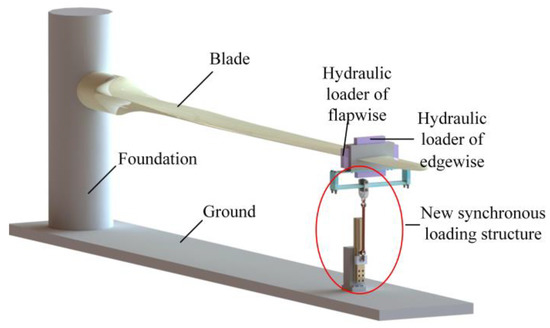
Figure 14.
A newly designed biaxial force decoupling device.
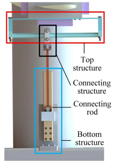
Figure 15.
New synchronous force decoupling structure.
As shown in Figure 16 the top structure consists of an upper rail, an under rail, fastening bolts, connecting bolts and nuts. The upper rail is fixed on the fixture by fastening bolts, and the upper rail and the lower rail are fixed by connecting bolts and nuts.
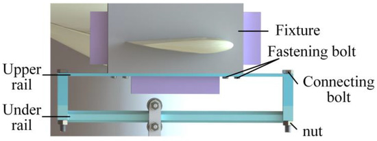
Figure 16.
Top structure.
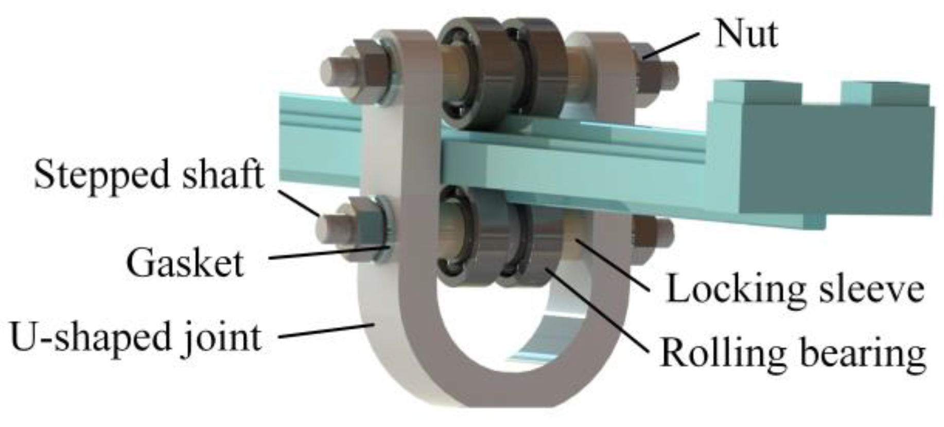
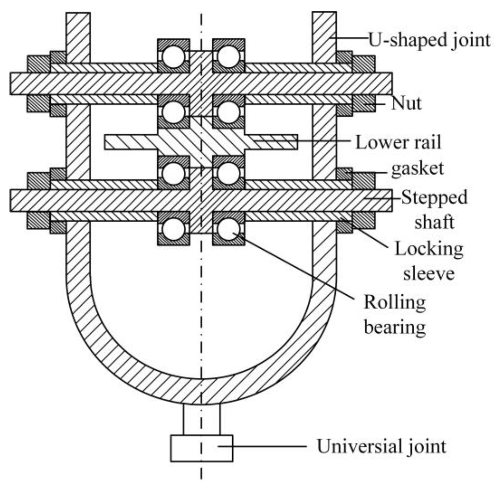
As shown in Figure 17 and Figure 18, the connecting structure consists of rolling bearings, U-shaped joint, stepped shafts, locking sleeves, gaskets and nuts. The whole connecting structure ensures which moves vertically along with the lower rail through the upper and lower pairs of rolling bearings, while the horizontal movement of the lower rail is converted into the autorotation movement of the outer ring of the rolling bearing that ensures that the connecting structure and the bottom structure do not move horizontally. In the connecting structure, the connecting shaft is fixed by a nut. The inner ring of the fixed rolling bearing and the locking sleeve are adopted to transmit the fastening force generated after the nut is tightened. The connecting structure is connected with the connecting rod through a universal joint.

Figure 17.
Connecting structure.
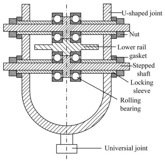
Figure 18.
Partial sectional view of connecting structure.
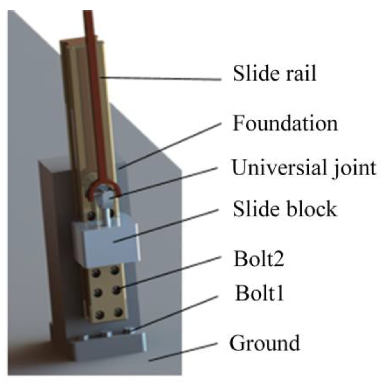
As shown in Figure 19, the bottom structure consists of a foundation, bolts, slide rail, and slide block. The foundation is fixed on the base by bolt 1, the slide rail is fixed on the base by bolt 2, and the slide block is fixed with the connecting rod by universal joints.
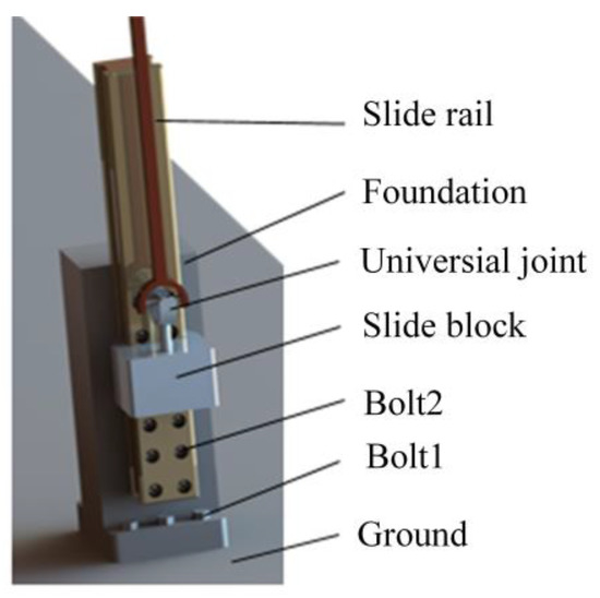
Figure 19.
Bottom structure.
3.2. Dynamic Characteristics Analysis of the New Force Decoupling Device
During the test, the total mass of the blade, fixture, vibration exciter, and top track is denoted as , and the total mass of the connecting rod, slide block, extra mass block, and the connecting structure shown in Figure 18 is denoted as Force diagrams of and are shown in Figure 20 and Figure 21, respectively.

Figure 20.
Force diagram of M.
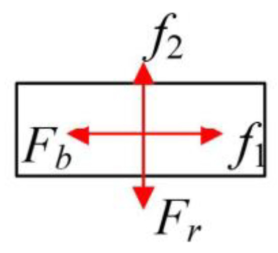
Figure 21.
Force diagram of m.
Dynamic analysis:
where and is exciting forces exerted on by the flap-wise vibration exciter and the edgewise vibration exciter, is the counterforce exerted by the push rod on the foundation , is the counterforce exerted by the base on in the edgewise direction, is the rolling friction between the rolling bearing and the top rail, and is the rolling friction between the slide block and the lower rail. and are the edgewise displacement and flap-wise displacements of the blade, and are flap-wise damping and edgewise damping of the blades, respectively, and and are the flap-wise stiffness and edgewise stiffness of the blade, respectively.
According to Equation (20):
where , and satisfy the following relationships:
where and are the amplitudes of the flap-wise excitation force and the edgewise excitation force, respectively, is the flap-wise natural frequency of system, is the edgewise natural frequency of the system, and and are the rolling friction coefficient and the sliding friction coefficient, respectively. According to the existing processing method, the minimum industrial friction coefficient can be decreased as low as 0.001 [38]. and are the flap-wise damping ratio and edgewise damping ratio of the system, respectively.
Substituting Equation (22) into Equation (21) leads to:
The product of friction coefficients is extremely small, so that the friction force can be neglected relative to the exciting force exerted by the exciter, so (23) can be simplified as:
According to Equation (24), the edgewise and flap-wise trajectories are:
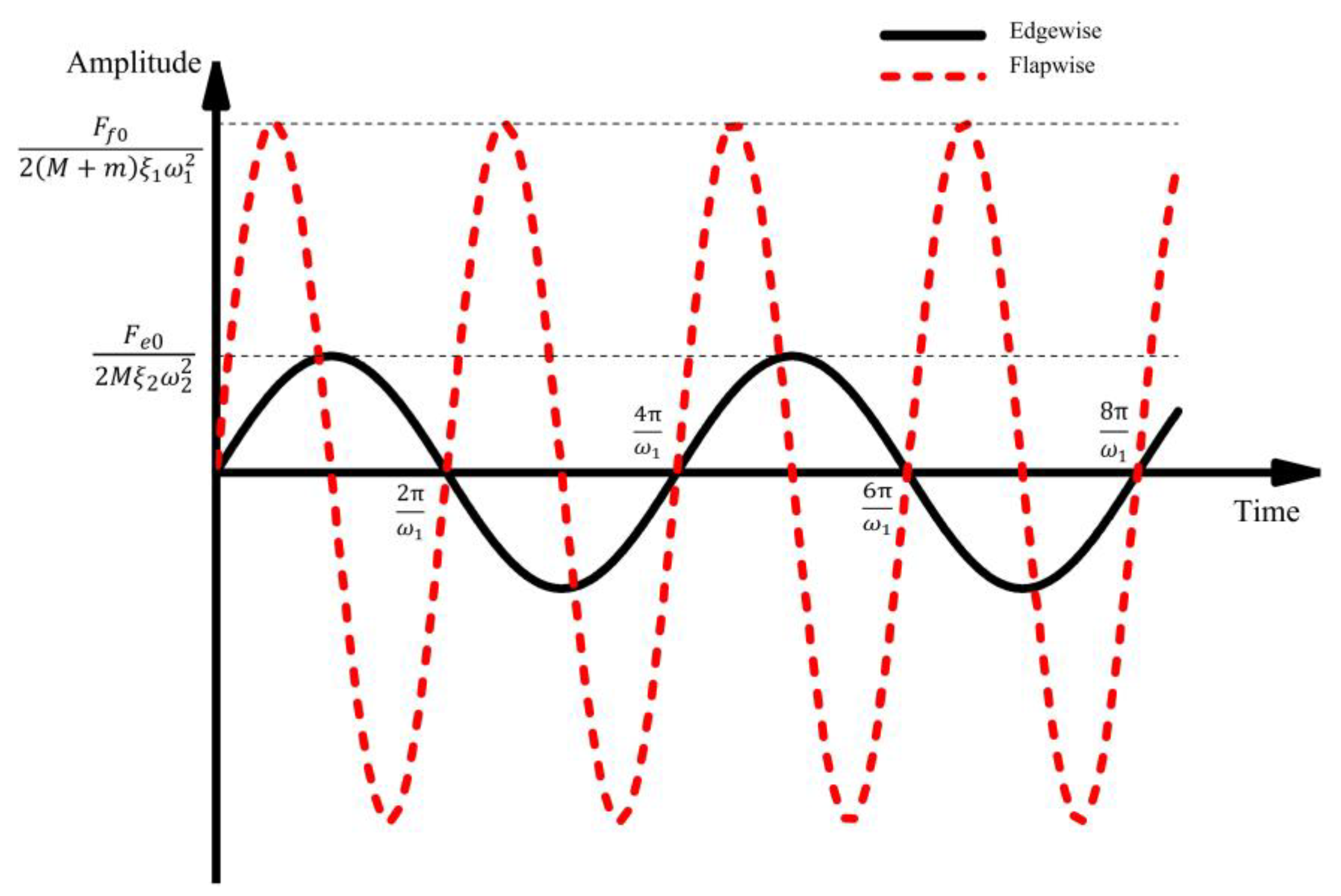
Figure 22 and Equation (25) show that the extra mass added flap-wise has no effect on the movement of edgewise, and the blade vibrates sinusoidally in two directions. Therefore, the bending moment-matching in the biaxial fatigue test using the newly designed device can be realized according to the following ideas: Firstly, determine the installation positions of the flap-wise and edgewise mass block and ensure that they are in the same position as much as possible. Secondly, according to the optimization algorithm, the optimal quality of mass block in the flap-wise and edgewise directions is obtained, which obviously cannot be completely the same. Therefore, for sections with unequal added mass in two directions, a new synchronous force decoupling structure needs to be set on the side with larger added mass to load the difference between the added mass in two directions. Finally, set the actual installed mass of the section on the blade to the smaller value of the required mass in both directions, and set the mass of the slider at each position as the mass difference between the two directions, and the influence of the bending moment of the mass in the other direction can be eliminated.

Figure 22.
Schematic diagram of blade vibration track in biaxial fatigue test.
Figure 23 shows a complete cycle of the newly designed device applied to a biaxial synchronous test.
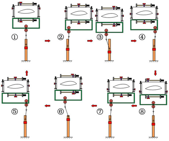
Figure 23.
Movement process of blades in a single cycle when using new force decoupling device.
3.3. Error Analysis of New Force Decoupling Device
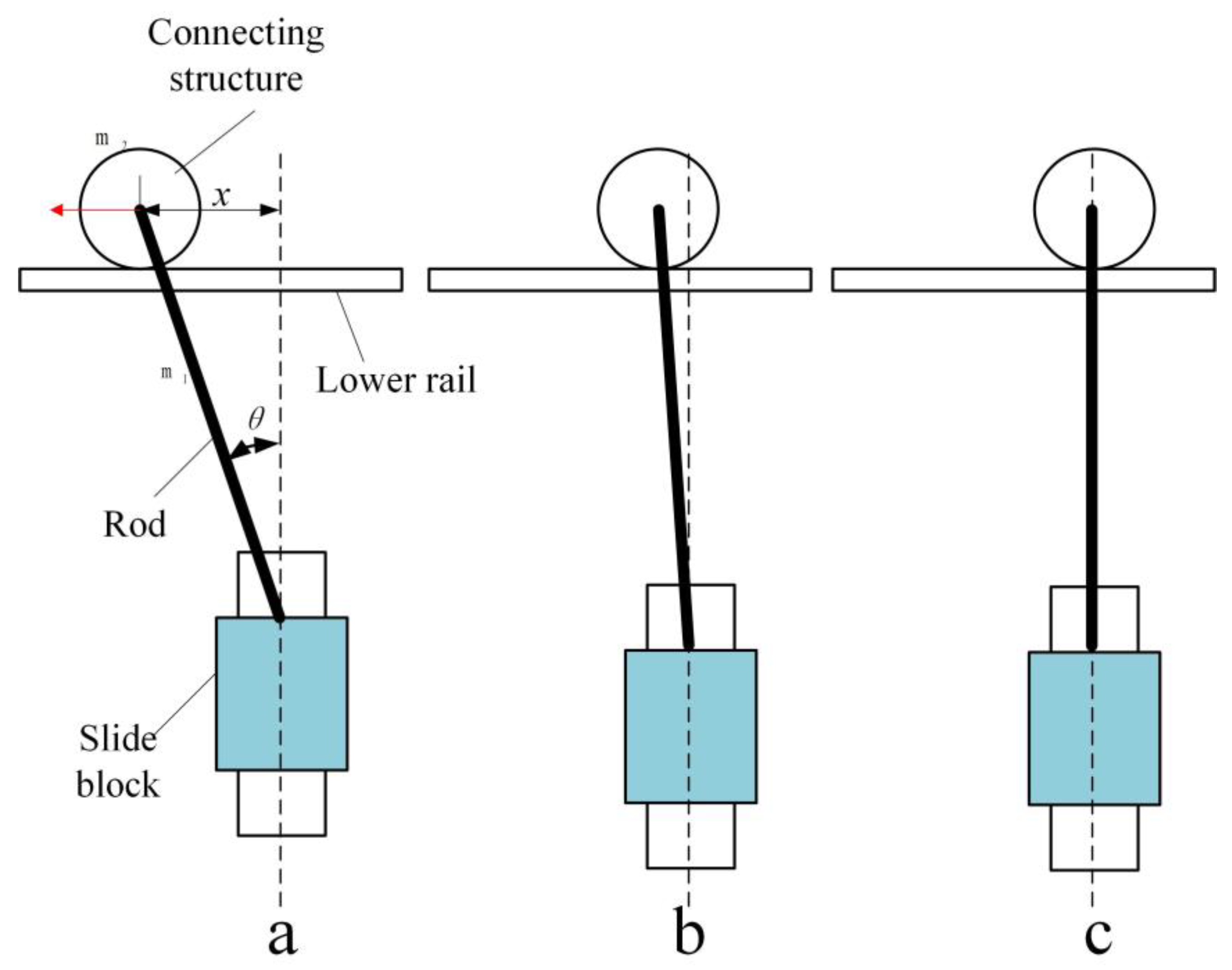
The error of the new synchronous force decoupling device is mainly caused by the friction between the bearing and the lower rail. Assuming infinite friction force, the generation mode of the bending moment error is the same as the virtual-mass type, as shown in Figure 24a. Assuming that the friction force is infinitesimal, the device has no bending moment-matching error according to the ideal situation, as shown in Figure 24c. When that roll bearing rotates normally, there is less friction between the bearing and the lower rail. Furthermore, the connecting rod has a smaller amplitude deviation, as shown in Figure 24b. In fact, the ideal situation does not exist. According to the existing treatment method, the industrial minimum friction coefficient can be treated as low as 0.001 [38]. The following analysis is conducted under the two conditions of infinite friction force and the normal rotation of the rolling bearing.

Figure 24.
Horizontal force diagram of connecting structure. (a–c) are infinite friction, normal friction and no friction respectively.
- (1)
- When the rolling bearing rotates normally.
Under the action of friction, both the connecting rod and the connecting structure will move horizontally. For the convenience of calculation, the connecting rod mass is equivalent to the connecting structure shown in Figure 17 according to the principle of energy conservation:
where is the mass of the connecting rod, is the mass of the connecting structure, is the equivalent mass of the connecting rod and the connecting structure, is the speed of the rod, is the speed of the connecting structure.
Furthermore, and satisfy the following relationship:
Substituting Equation (27) into Equation (26):
According to Equation (25) and Equation (28), the acceleration of the equivalent mass in the horizontal direction under the action of friction is:
Assuming that the deflection angle has no effect on the blade motion, the maximum horizontal displacement of the equivalent mass under the action of friction force in a quarter edgewise period is:
The maximum deflection angle of the connecting rod is,
where is the length of the connecting rod.
The is farthest from the mass , so the change in the connecting rod angle has the most obvious influence on the bending moment of the blade root. Therefore, taking the blade root section as an example, the ratio of the flap-wise bending moment and the ratio of the edgewise bending moment when the deflection angle of the connecting rod is maximum and when the connecting rod is not deflected is as follows:
where is the ratio of the flap-wise bending moments, is the ratio between the edgewise bending moments, is the distance from mass to blade root, is the flap-wise bending moment produced by mass , is the flap-wise bending moment produced by mass .
Take the same 60 m-long blade [36] as an example to calculate, the connecting structure mass is 30 kg, the connecting rod mass is 40 kg, the total mass of the connecting structure, connecting rod, slide block, and extra mass block is 400 kg; the amplitude of flap-wise at the installation position of extra mass block is 3.69 m; and the frequency of flap-wise is 2.64 rad/s. The rolling friction coefficient is 0.001, and and are 3852 kN·m and 5250 kN·m, respectively. Because the length of the connected rod must be longer than the flap-wise amplitude , the length of the rod must be longer than 3.69 m to prevent the blade from colliding with the guide rail. According to the above data, the variation trend in the bending moment error in two directions at the limit position with the variation in rod length is shown in Figure 25.
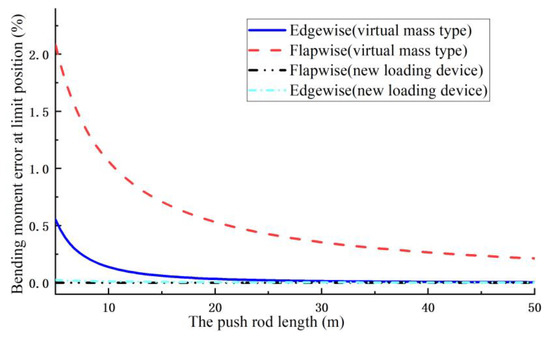
Figure 25.
Changing trend of bending moment error of two devices with increasing rod length.
- (2)
- When the rolling bearing cannot rotate
Compared with the situation that the rolling bearing rotates normally, when the rolling bearing cannot rotate, as shown in Figure 21a, the connecting structure can be regarded as rigidly connected with the lower rail, and the deflection angle of the connecting rod is larger when the blade is in the extreme position. In this condition, the bending moment error on the blade root can be calculated by Equations (32) and (33). Taking the same 60 m long blade as an example to check the bending moment error, it can be obtained that the change trend in the bending moment error in both directions of blade root with the increase in the rod length is the same as that of virtual-mass type when the blade is in the extreme position, as shown in Figure 10.
To sum up, when the rolling bearing rotates normally, it can be seen from Figure 25 that compared with the virtual-mass device, the bending moment error caused by the rod length of the new biaxial synchronous force decoupling device is obviously reduced, which is basically negligible. In addition, compared with the virtual-mass device which uses hydraulic cylinder to apply exciting force to the blade, the device uses motor-driven mass to apply exciting force to the blade, which makes the overall structure simpler and of lower cost.
Although the newly designed device improves the loading force coupling problem of virtual mass type, in this case analysis, when the edgewise movement reaches the limit position, the newly designed device may apply torsional load to the blade. As a new structure, the newly designed device provides a new idea for the test scheme in practical engineering application, and the torsion problem caused by it needs further research to be eliminated.
4. Fast Moment-Matching Method and Case Study for Biaxial Synchronous Loading Conditions
4.1. Development of the Moment-Matching Method
In the loading process of the resonant fatigue test, it is necessary to install mass blocks with a specific quality at different positions of the blade while adjusting the bending moment distribution of the blade as close to the target bending moment as possible. The difficulty of this method lies in the selection of the quantity, position, and quality of the mass block. If the selected quantity, quality, and location are unreasonable, it will not only unnecessarily increase the energy consumption but also enlarge the bending moment error. In order to quickly and accurately determine the bending moment-matching scheme, new methods have been applied continuously. The scheme evolution of bending moment-matching mainly has the following stages.
Manual trial and error method and experiments:
The initial loading scheme is screened manually, the bending moment-matching effect of the loading scheme is verified by experiments. An ideal loading scheme is obtained by trial and error and test [35]. It takes a lot of time and manpower to confirm the loading scheme by this method, which does not meet the requirements of accurate and efficient tests.
Using FEA instead of tests:
With the maturity of computer simulation technology, the FEA (Finite Element Analysis) begins to replace manual experiments [39]. NREL [40] proposed that using a finite element shell model to analyze the blade with enough nodes to describe the cross-section shape of the blade, which could more accurately simulate the actual vibration direction of the blade much more accurately.
The use of FEA instead of a manual test reduces a lot of manpower. However, the method of manually screening the mass block schemes still needs repeated trial and error, which is inefficient and difficult to obtain ideal bending moment-matching effect.
Using PSO instead of manual screening
Zhang et al. [41] took a 38 m-long blade shell model as the finite element analysis object and obtained the optimal moment-matching scheme to minimize the moment error of the key section of the blade by PSO (Particle Swarm Optimization), which verified the effectiveness of PSO+FEA scheme.
The shell model can accurately express the vibration direction of the blade, but the structure is complex and requires a large amount of calculation. In the optimization process of Zhang et al.’s PSO work, it is necessary to use the finite element model for tens of thousands of repeated operations [41]. However, when FEA is used in the calculation of wind turbine blades, a single FEA operation usually takes several minutes [42,43,44,45], and the time cost of superposition is enormous. In addition, uncertain time factors such as FEA physical object modeling and grid drawing should also be considered, as well as the ability requirements of technicians in this part of the operation.
Using TMM instead of FEA:
The TMM (Transfer Matrix Method) was established in the 1920s to study the one-dimensional linear vibration of elastic components, and it has since been applied to the research fields of aircraft wings, rocket launching systems, wind turbine towers, and so on, with the advantages of simple programming, fast calculation, and relatively accurate prediction results [46,47,48].
The fatigue testing process of wind turbine blades can be simplified as a one-dimensional linear vibration problem of an elastic component corresponding to the TMM, and the discretized key sections and physical parameter definitions provided at the beginning of blade design also fit the calculation method of the TMM. In the previous work before this paper, the results published by the authors have verified the feasibility and accuracy of using the TMM to calculate the bending moment of blade section. The predicted bending moment calculated by the TMM is less than 1% compared with the experimental bending moment measured [49]. M. Q. Han et al. [50] improved the TMM by using the particle swarm optimization algorithm, and the results showed that the moment calculation ability was more accurate than that of the FEA. What is more, when using a personal notebook computer with common configuration, the TMM single solution time is less than 3 s. Compared with the minutes required by FEA [42,43,44,45], the time benefit in a large number of repeated calculations is huge. Therefore, using the TMM instead of FEA to calculate the bending moment distribution can not only ensure the calculation accuracy but can also greatly speed up the calculation time.
In addition, the TMM process is simple. When the TMM method is used to calculate the bending moment and solve the optimal mass block loading scheme, the whole optimization calculation can be completed only by inputting the basic parameters after the discretization of blades, which greatly reduces the technical requirements for operators compared with FEA. Theoretically, the operators only need certain basic knowledge and can skillfully use the computer.
The basic mechanism of using the TMM to calculate the bending moment is as follows: discretize the model, simplify the blade into a long rod, and cut it into several elements, each of which includes a massless rod and a concentrated mass. In this way, the calculation of the whole system is decomposed into the operation of transfer matrix and state matrix among each unit. Then, the transfer matrix and the state matrix are integrated to obtain the bending moment of each key section.
Using TMM instead of FEA can quickly and accurately calculate the set section bending moment of blades, which may more practically meets the engineering application requirements.
4.2. Applying TMM+PSO for Fast Moment-Matching, the Case Study
4.2.1. Apply TMM to Fast Bending Moment Calculation
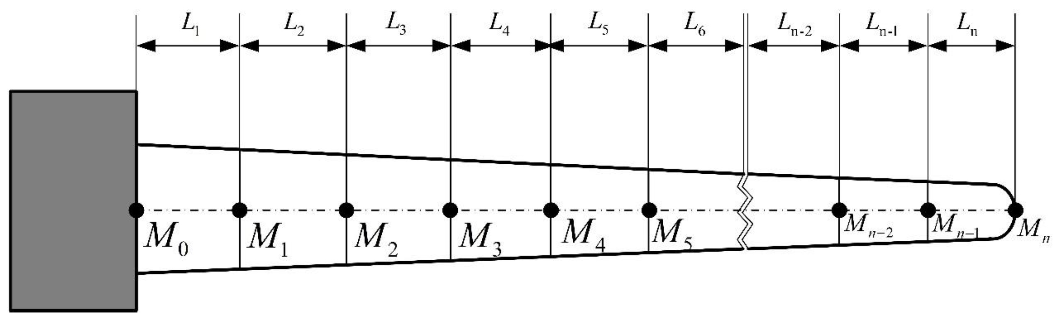
As shown in Figure 26, the blade parameters are discretized at the factory stage, and the entire blade is divided into segments along the axis. This division method is very suitable for the calculation requirements of the TMM.

Figure 26.
Blade segmentation model [49].
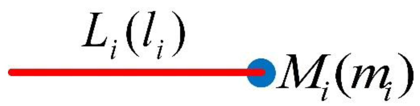
According to the general research method of the TMM, each blade segment can be simplified into a massless length part and a lengthless mass part . The length and mass are and , respectively. As shown in Figure 27, the right side of the length part and the left side of the mass part are the same section.

Figure 27.
One of blade segments model.
According to the general method of the TMM, the state of the set section can be represented by the state matrix :
where , , , and are the deflection, rotation angle, bending moment, and shear force, respectively. Furthermore, use to represent the state matrix of the right cross-section of blade unit .
According to the general calculation method of the transfer matrix method, the state matrix relationship of the right sections of the adjacent blade elements is:
where is defined as the blade segment transfer matrix, and its expression can be listed as [51]:
where represents the natural frequency of the blade, represents the section stiffness of blade segment , and represents the additional mass of the set section.
According to the relationship between adjacent transfer matrices of Equation (34), it is easy to obtain:
where is defined as the global transfer matrix:
Analyzing the blade model shown in Figure 26, the blade root deflection and deflection angle are both 0 during the blade test, and the blade tip bending moment and shear force are both 0 because no additional mass is placed on the blade tip [50]. Rewrite the complete expression of (36) as:
Analyze the above equation to obtain:
Analyze the system of equations and obtain the following relationship:
It can be obtained from Equations (35) and (36) that, in addition to the known blade parameters, the only factor that affects is the blade natural frequency , so the blade natural frequency can be easily obtained by the above equation. In Equation (40), once the natural frequency of the blade is determined, the blade segment transfer matrix and the system transfer matrix can be completely determined. Using the transfer matrix, the state matrix of each set section can be obtained by Equation (35), and the set section bending moment can be obtained.
It is easy to find that through the above method, as long as the length, mass quality, section stiffness, and other parameters of the blade segmentation model are known, the computer can quickly calculate the bending moment of each set section.
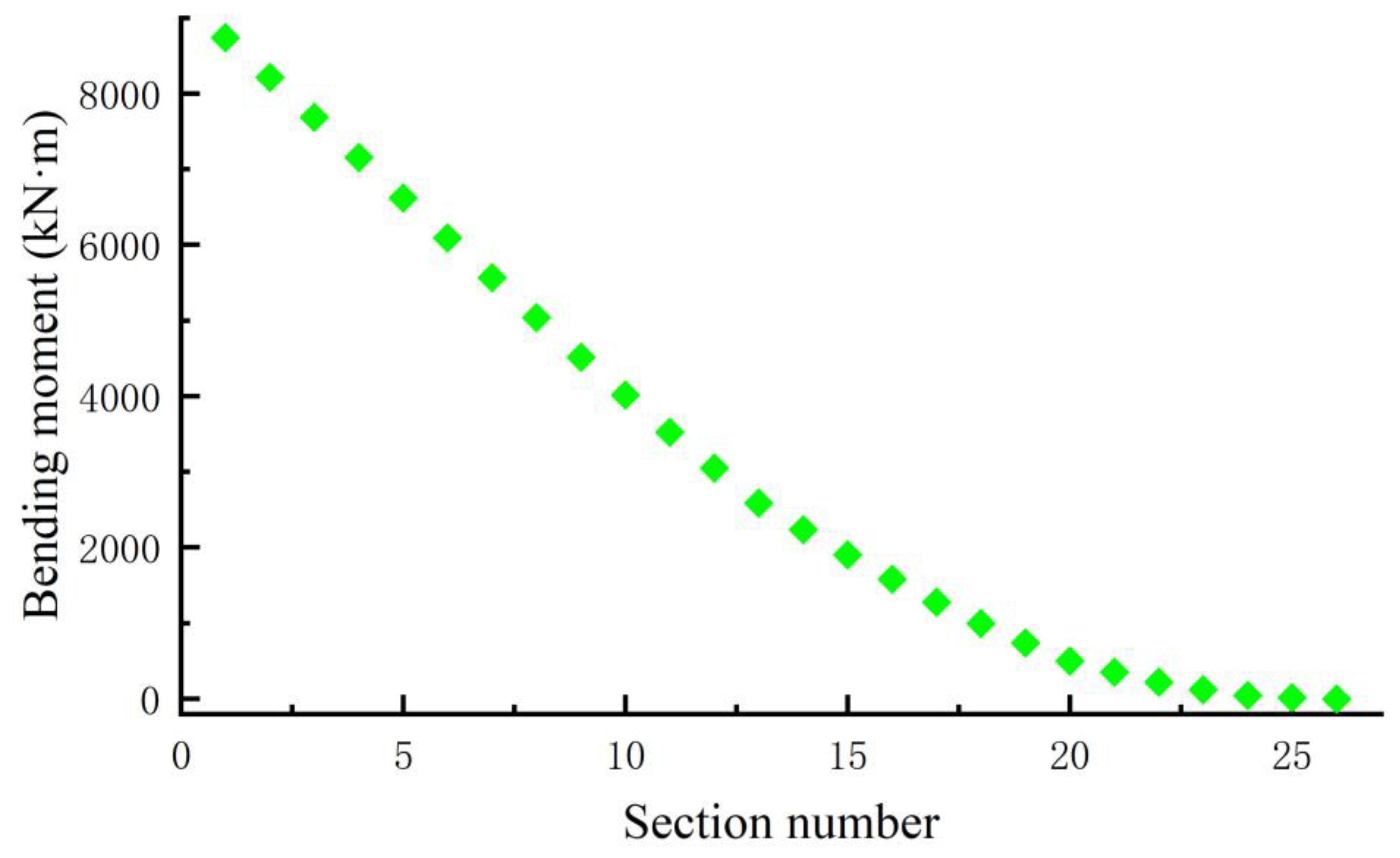
Taking a 60 m-long blade [36] provided by NREL as an example, the TMM is used to calculate the bending moment distribution of its set section. According to the factory setting of the blade, the key flap-wise and edgewise section is taken as the first 70% of the blade length, that is, 0~42 m. The blade includes 25 units.
Taking flap-wise bending moment calculation process as an example, using TMM to calculate the bending moment distribution of the set section, it can be calculated in turn that:
Furthermore, the bending moment distribution of the set section of the blade can be calculated, as shown in Figure 28.
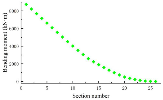
Figure 28.
Bending moment on blade sections.
4.2.2. Apply PSO to Fast Bending Moment Matching
The PSO algorithm was first proposed by J. Kennedy and R. Eberhart [52] in 1995, which was inspired by the information flow and social behavior observed in birds and fish schools. The main idea of applying the PSO algorithm to practical examples is to design a kind of particle without mass to simulate birds and schools of fish, where each particle has only two attributes: position and speed. Each particle searches for the optimal solution independently in the search space and records it as the optimal solution of the current particle. All particles share the current optimal solution and screen out the global optimal solution. All particles constantly adjust and update their speed and position according to the current and global optimal solutions and update rules. After a certain number of iterations, all particles gather near the global optimal solution, finally obtaining the global optimal solution [53].
The biaxial loading mode of the new synchronous force decoupling device for fatigue test designed in this paper is resonance type, and it is necessary to reduce the natural frequency of the blade by installing mass blocks on the blade to adjust the actual bending moment distribution of the blade to approach the target bending moment. The authors put forward a scheme to find the optimal moment-matching method by using PSO and the TMM, which is applied to the 60 m-long blade for verification. The application of PSO in bending moment-matching optimization mainly includes four aspects: design variables, constraints, objective functions, and optimization process. In order to ensure that particles meet the loading requirements and speed up the solution, it is necessary to preliminarily determine the installation position or position range of mass block by human intervention before formal solution.
- (1)
- Human intervention
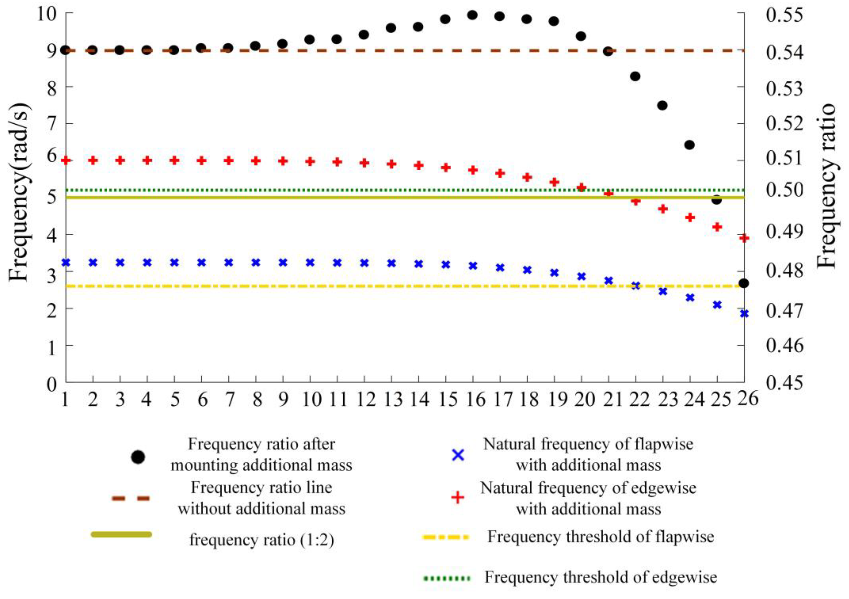
As mentioned in Chapter 1.2, the frequency ratio between the flap-wise resonance and the edgewise resonance of the blade in the range of 50–60 m-long tends to be 1:2, so the frequency ratio of this design is selected as 1:2. When the blade is not installed with a mass block, the ratio of the natural frequency of flap-wise and the natural frequency of edgewise calculated by the TMM is about 1:1.85, so it is necessary to preliminarily determine the installation position of mass block.
The 900 kg mass block is installed on different sections of the blade for testing, and the natural frequency and frequency ratio of the blade are obtained as shown in Figure 27, which shows that:
- When the mass block is installed in the range of blade sections 0–19, the frequency ratio increases;
- When the installation position is within the range of blade sections 20–23, the frequency ratio decreases but is still higher than 1:2;
- When the mass block is installed on blade sections 24 or 25, the frequency ratio is lower than 1:2, but the natural frequency of the blade is lower than the frequency threshold.
Therefore, the mass block used to adjust the natural frequency must be installed within the range of blade sections 20–23, and the mass block used to adjust the flap-wise natural frequency must be greater than that of edgewise, so that the frequency ratio of 1:2 can be realized on the premise of ensuring that the system frequency is greater than or equal to the frequency threshold.
Considering that the stiffness of blade sections 22 and 23 is small, the mass of the largest mass block that can be installed is small, and compared with blade section 20, the natural frequency of the blade changes more when the mass block with the same mass is installed in blade section 21, section 21 is therefore selected as the installation position of the mass block to adjust the natural frequency of the blade.
In addition to adjusting the natural frequency of the system, it is necessary to install mass blocks to adjust the local bending moment of the blade. According to Figure 29:
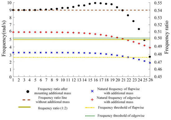
Figure 29.
Natural frequency and frequency ratio of the system when the mass block with the same mass is installed at different positions of the blade.
- d.
- The bending moment produced by the mass block in the range of sections 0–7 is very small, which cannot play a regulating role.
- e.
- Installing a mass block in the range of blade sections 8–12, the system frequency does not change much.
- f.
- Installing a mass block in the range of blade sections 13~18, the system frequency will change slightly.
- g.
- When the mass block is installed behind blade section 18, the system frequency will change greatly.
Therefore, the mass block can be selected at the same position at the range of blade sections 8~12 to adjust the local bending moment of blades in both directions at the same time, and different mass blocks can be installed at the range of blade sections 13~18 to adjust the local bending moment of blades.
Through the human intervention of the above steps, the installation position and position range of the mass blocks are determined.
As the excessive number of mass blocks will make the blade structure redundant and cause redundant energy consumption, the number of mass blocks should be reduced as much as possible while ensuring that the test bending moment on the blade meets the target bending moment. So, firstly, the number of mass blocks should be selected as two. If the bending moment-matching cannot be completed within the preset mass blocks while the number of mass blocks is two, the number of mass blocks should be taken as three. If the optimal result still cannot be obtained, the number of mass blocks should be taken as four, and so on, until the optimal result is obtained.
- (2)
- Design variables
The flap-wise root bending moment and edgewise root bending moment must be determined before solving the bending moment on the key section of blade. The purpose of the optimization program for bending moment-matching in biaxial fatigue test is to obtain the scheme of mass blocks that minimizes the sum of bending moment errors of flap-wise and edgewise sections of key blades when the position and number of mass blocks are known. Therefore, the root bending moment of flap-wise and edgewise and the mass of mass blocks are taken as design variables in this design. Set the number of mass block as . As the installation positions of flap-wise and edgewise mass blocks are the same, the design variable is:
where ( = 1, …, R) is the mass of the number i mass block installed flap-wise, and ( = 1, …, R) is the mass of the number i mass block installed edgewise.
- (3)
- Constraints
Installing mass blocks on the blade to adjust the bending moment will reduce the natural frequency of the system, resulting in an increase in the test period. In order to prevent the frequency from being too low, it is necessary to set a frequency threshold for the natural frequency of the system. Since the biaxial bending moment-matching involves two directions, it is necessary to set a threshold for the frequencies in both directions. If the mass of the mass block installed on the blade is too large, it will cause structural redundancy and consume redundant energy, while, if it is too small, it will not play the role of mediating the bending moment, so the mass of the mass block also needs to be limited. In addition, as a design variable, the blade root bending moment also needs to be limited, because if the bending moment of the blade root is too large or too small, the bending moment of the blade cannot be matched within the given mass block range, so the program constraint conditions are as follows:
where and ( = 1, …, R) are the lower and upper mass limits of the flap-wise mass block i, respectively; and ( = 1, 2, …, R) are the lower and upper mass limits of the edgewise mass block ; and , , and are the flap-wise natural frequency, edgewise natural frequency, flap-wise frequency threshold, and edgewise frequency thresholds, respectively. , , , and are the lower limits and upper limits of the root bending moment in the flap-wise and edgewise directions, respectively.
- (4)
- Objective function
In order to bring enough damage to the blade, the test bending moment in the target area must be greater than or equal to the target bending moment. At the same time, in order to avoid excessive damage to the blade, the bending moment of the blade should be as close as possible to the target bending moment. To achieve this goal, Zhang et al. [41] compared the optimization results of the sum of absolute error squares and the sum of relative error squares of bending moments of key sections as objective functions. The latter required that the relative error of bending moments of key sections should not exceed 20%, the results showed that the moment error obtained by the latter as objective function was smaller. Considering that the square error of section bending moment is small and difficult to compare, in this paper, the sum of the standard deviation of relative errors of bending moments of key sections, rather than the sum of squares, is used as the objective function. In order to obtain more accurate results, the relative errors of the bending moments of each section are no less than 0 and no more than 10%. Setting the number of key sections of blades as , the objective function is as follows:
where , and (j = 1, 2, …, N) are the calculated bending moment, target bending moment, and bending moment errors of section flap-wise, and , and (j = 1, 2, …, N) are the calculated bending moment, target bending moment, and bending moment errors of section edgewise. Moreover, and are the lower limit and upper limit of the bending moment error, respectively.
- (5)
- Optimize the process
The mathematical description of the PSO-based biaxial bending moment optimization matching program is as follows:
- (a)
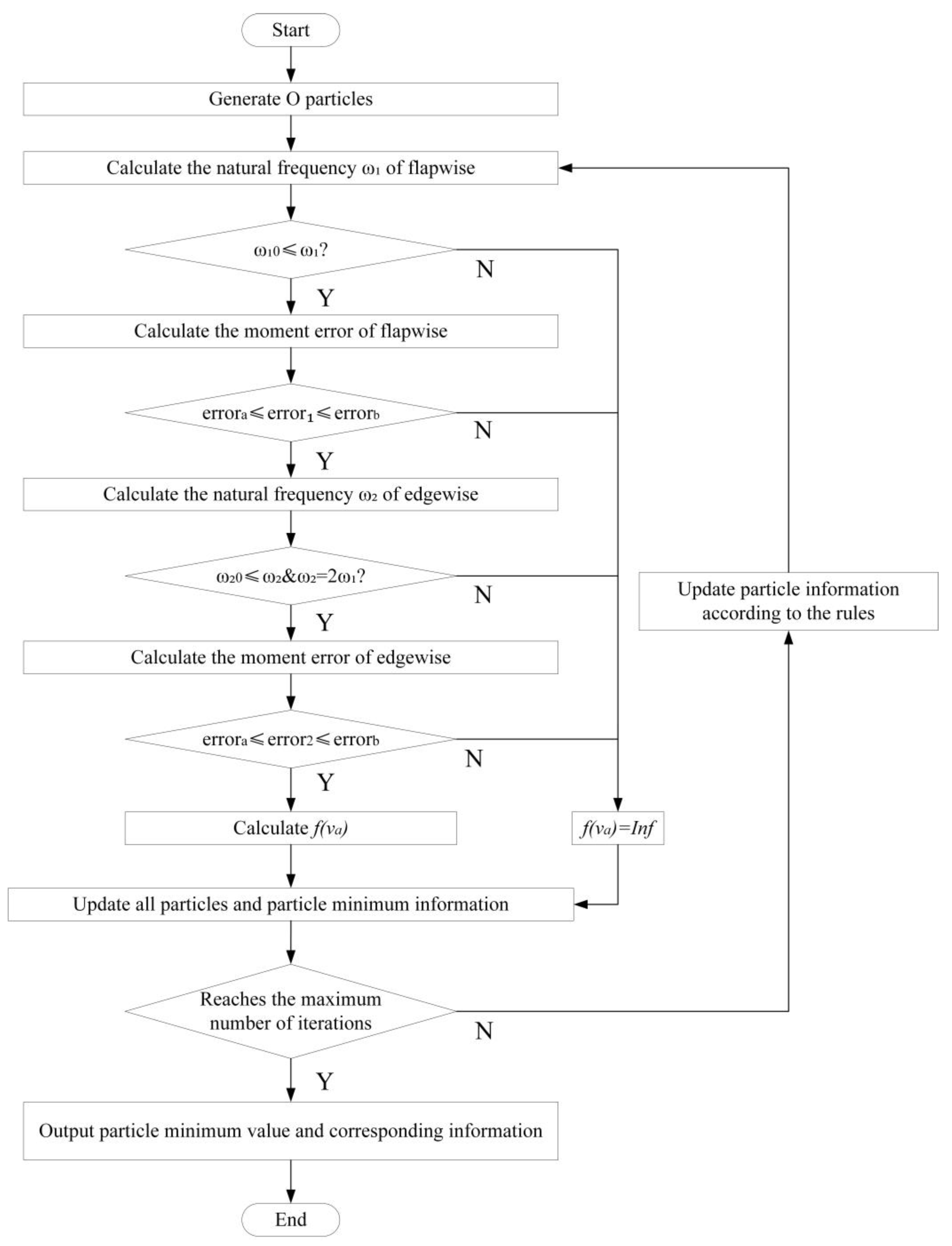
- Set the number of mass blocks as and the number of key sections as . Then, randomly generate schemes, including mass block and root bending moment within the constraint range shown in Equation (42), i.e., particles. Combined with blade parameters, the first-order natural frequency of flap-wise particles can be calculated by the transfer matrix method.
- (b)
- Judge the relationship between the frequencies and : if , then the = Inf; if , the flap-wise bending moment (j = 1, 2, …, N) of the key section of the particle can be calculated by the transfer matrix method, and the flap-wise bending moment of the key section of the particle can be calculated by substituting Equation (43). Then, judge whether meets the error requirement: if yes, continue to step (c). If not, .
- (c)
- Calculate the magnitude relationship between the first-order natural frequencies and edgewise of the particle. If and , the edgewise bending moment (j = 1, 2, …, N) of the key section of the particle can be calculated by the transfer matrix method, and the flap-wise bending moment of the key section of the particle can be calculated by substituting Equation (43). Then, judge whether meets the error requirement, if yes, calculate the ; otherwise, the .
- (d)
- Update the minimum value of each particle and the minimum value of all particles.
- (e)
- Judge whether the number of iterations reach the maximum number, and if so, output the minimum value of all particle objective function values and the corresponding optimal scheme. If not, update the particle information and repeat steps (b) and (c) until the iteration times meets the requirements.
The specific flow of calculating the bending moment by PSO is shown in Figure 30.

Figure 30.
Flow chart of fast calculation method for optimal matching of bending moment in biaxial fatigue test based on PSO.
Suppose that the state property of particle after iteration is:
where = 1,., , refer to the position, velocity, individual optimal position, and global optimal position of particle after the t iteration, respectively.
The velocity and position updating equation of particle in the t + 1 iteration process is as follows:
where is the inertia weight, and are random numbers distributed between (0,1), and are learning factors, and usually = = 2.
Take the 60 m-long blade used by NREL [36] as an example to conduct a case analysis of the bending moment matching optimization. When the number of mass blocks are two, three, and four, the program does not obtain the optimized result, and when the number of mass blocks is five, the parameters can be set as in Table 1.

Table 1.
Parameter Settings.
The optimal scheme obtained by the bending moment-matching optimization program is shown in Table 2, while the calculated bending moments of the flap-wise and edgewise blades after optimization are shown in Figure 31.
Table 2.
Convergence results of the case study.

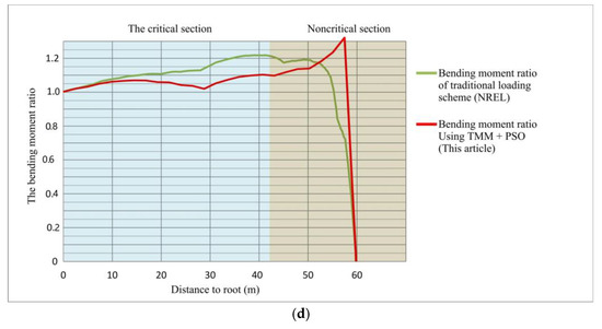
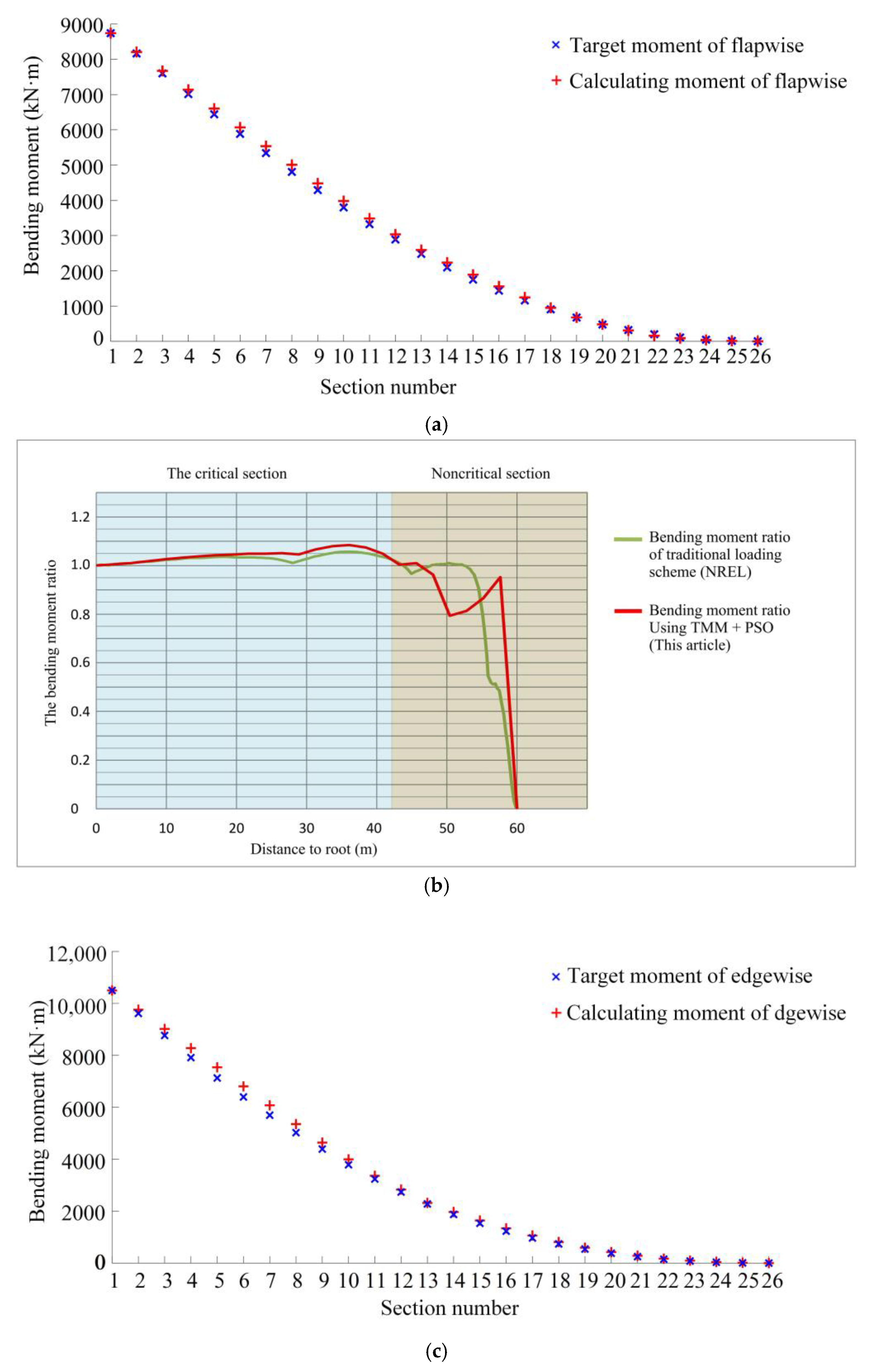
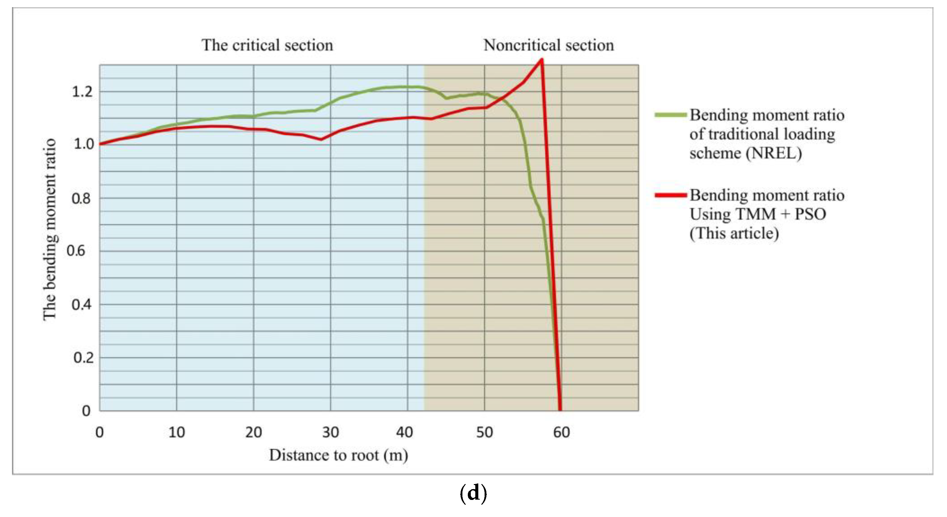
Figure 31.
Comparison between optimization result and target bending moment. (a) flap-wise bending moment distribution; (b) Ratio of predicted bending moment to target bending moment in flap-wise; (c) edgewise bending moment distribution; (d) Ratio of predicted bending moment to target bending moment in edgewise.
Figure 31 shows that the moment error of the key section flap-wise is basically less than 5% and the maximum moment error of the flap-wise key section does not exceed 9%. The moment error of most key sections is less than 7% in edgewise and the maximum moment error of key sections in edgewise is less than 10%. Therefore, the optimal design of the bending-matching moment meets the requirement that the frequency ratio is 1:2, ensuring that the test bending moment of key section meets the requirement of bending moment error.
Due to the particularity of biaxial resonance loading, it is required that the masses in both directions should be placed in the same section as much as possible, which leads to the selection of the section not completely depending on the matching effect in one direction. That is, the effects in both directions will influence each other. Compared with the loading scheme used by NREL, the actual-target bending moment ratio of the loading scheme calculated by TMM+PSO in the key section in flap-wise is closer, and it does not exceed 1.1. The overall matching effect of the edgewise key section is better than that of NREL, and the maximum bending moment ratio is reduced from above 1.2 to less than 1.1.
In this case, the 60 m-long blade used is evenly divided into 25 units with a length of 2.4 m. The computational characteristics of the TMM+PSO determine that the loaded mass must be placed at the preset section, and the optimal matching scheme is also based on this setting. In this example, the matching effect of the loading scheme can also be improved by refining the blade unit, which could make the position and quality of the final loading scheme more reasonable. Accordingly, it will take more time to solve the scheme.
5. Conclusions
With the development of the application range of the wind turbine and the continuous increase in blade size, the biaxial fatigue test is more and more popular as a more accurate and reasonable method than the uniaxial fatigue test.
This paper firstly reviews the process of establishing the target moment, which includes the basic steps of load calculation, load spectrum compilation, cumulative damage modeling, Goodman correction, and equivalent load determination. Then, three representative loading devices are introduced and compared from the perspective of the energy consumption relationship and the loading force coupling relationship, which is forced loading, hybrid loading, and virtual mass loading, respectively. The energy consumed by the three devices decreases in turn. The loading forces in both directions of forced loading and virtual mass loading are coupled with each other. The loading force of hybrid loading edgewise will affect the flap-wise loading. For this, a new force decoupling design is proposed in this paper, which leaves out the excess flap-wise mass through the bottom structure, avoiding influencing the edgewise test, thus realizing biaxial resonance loading. The additional error analysis shows that when the rolling bearing rotates normally, the loading forces of the two axes hardly influence each other, which ensures that the actual stress direction of the blade is basically consistent with the test direction. Therefore, the bending moment error can be almost ignored. However, the newly designed device may produce torque to the blade at the limit position of the shimmy, which still needs further research to eliminate.
In the future, a case discussion for quick moment calculation and matching using the TMM and PSO methods is proposed. This method has been proven to be superior to FEA in computational efficiency and professional dependency in previous work. A 60 m-long blade referred by NREL is taken as the research object for verification. The results show that the bending moment-matching scheme calculated by the TMM and PSO is better than the loading scheme proposed by NREL. The actual-to-target flap-wise bending moment ratio in key sections is almost the same, while the edgewise one is less than 1.1, which is better than the ratio of 1.2 in the traditional loading scheme provided by NREL.
Author Contributions
Conceptualization, writing—review and editing, supervision, project administration, funding acquisition, L.L.; validation, formal analysis, software visualization, M.Z.; methodology investigation and data curation, writing—original draft preparation, H.W.; resources, J.W. All authors have read and agreed to the published version of the manuscript.
Funding
This research was funded by the Shanghai Municipal Science and Technology Major Project (No.2021SHZDZX0100), Shanghai Municipal Commission of Science and Technology Project (No.19511132101) and the Fundamental Research Funds for the Central Universities (2022-1-ZD-04).
Conflicts of Interest
The authors declare no conflict of interest.
Nomenclature
| Symbol | Description |
| Number of stress cycles before material failure | |
| Parameters related to material properties, patterns, stress ratios, and loading modes | |
| Stress amplitude | |
| Amount of damage | |
| Load loading times | |
| Stress ratio | |
| Stress, material strength, conditioned fatigue limit | |
| The force exerted on the blade by the flap-wise and edgewise hydraulic loaders | |
| The angle between the flap-wise (edgewise) force and the vertical (horizontal) direction | |
| Displacement of edgewise direction and flap-wise direction | |
| Damping of the flap-wise direction and edgewise direction | |
| Stiffness of the flap-wise direction and edgewise direction | |
| Quality of blade | |
| Force amplitude of the flap-wise direction and edgewise direction | |
| Force loading frequency of the flap-wise direction and edgewise direction | |
| Natural frequency of the blade in the flap-wise direction and edgewise direction | |
| Damping ratio of the flap-wise direction and edgewise direction | |
| Maximum value at the excitation point of the flap-wise direction and edgewise direction | |
| Length of the hydraulic loader in the flap-wise direction and edgewise direction | |
| The actual force of the flap-wise direction and edgewise direction | |
| friction coefficient | |
| The moment error at the limit position of the flap-wise direction and edgewise direction | |
| Quality | |
| Speed | |
| Maximum horizontal displacement of equivalent mass | |
| Maximum deflection angle of the connecting rod | |
| Length of the connecting rod | |
| Distance of section i from the root section | |
| Transfer matrix | |
| Segment i transfer matrix | |
| First natural frequency | |
| Blade root bending moment | |
| Blade root shear | |
| The i row, j column of the transfer matrix H | |
| Blade root state matrix | |
| Quality of balancing mass | |
| Calculated bending moment of the section j flap-wise and edgewise | |
| Target bending moment of the section j flap-wise and edgewise | |
| Bending error of the section j flap-wise and edgewise | |
| Lower limit and upper limit of the bending moment error |
References
- Jonkman, J.M. Dynamics Modeling and Loads Analysis of an Offshore Floating Wind Turbine; University of Colorado at Boulder: Boulder, CO, USA, 2007. [Google Scholar]
- Jonkman, J.M.; Buhl, M.L., Jr. Loads Analysis of a Floating Offshore Wind Turbine Using Fully Coupled Simulation; National Renewable Energy Lab. (NREL): Golden, CO, USA, 2007.
- Jang, Y.J.; Choi, C.W.; Lee, J.H.; Kang, K.W. Development of fatigue life prediction method and effect of 10-minute mean wind speed distribution on fatigue life of small wind turbine composite blade. Renew. Energy 2015, 79, 187–198. [Google Scholar] [CrossRef]
- Toft, H.S.; Svenningsen, L.; Sørensen, J.D.; Moser, W.; Thøgersen, M.L. Uncertainty in wind climate parameters and their influence on wind turbine fatigue loads. Renew. Energy 2016, 90, 352–361. [Google Scholar] [CrossRef]
- Marino, E.; Giusti, A.; Manuel, L. Offshore wind turbine fatigue loads: The influence of alternative wave modeling for different turbulent and mean winds. Renew. Energy 2017, 102, 157–169. [Google Scholar] [CrossRef]
- Liu, G.; Wang, D.; Hu, Z. Application of the rain-flow counting method in fatigue. In Proceedings of the 2nd International Conference on Electronics, Network and Computer Engineering (ICENCE 2016), Yinchuan, China, 13–14 August 2016; Volume 67, pp. 232–236. [Google Scholar]
- Song, Y.; Li, C.; Wang, L. Rain-flow and reverse rain-flow counting method for the compilation of fatigue load spectrum. China Ocean. Eng. 2001, 3, 429–435. [Google Scholar]
- Tuller, S.E.; Brett, A.C. The characteristics of wind velocity that favor the fitting of a Weibull distribution in wind speed analysis. J. Appl. Meteorol. Climatol. 1984, 23, 124–134. [Google Scholar] [CrossRef] [Green Version]
- Kantar, Y.M.; Usta, I. Analysis of the upper-truncated Weibull distribution for wind speed. Energy Convers. Manag. 2015, 96, 81–88. [Google Scholar] [CrossRef]
- Epaarachchi, J.A.; Clausen, P.D. The development of a fatigue loading spectrum for small wind turbine blades. J. Wind. Eng. Ind. Aerodyn. 2006, 94, 207–223. [Google Scholar] [CrossRef]
- Ragan, P.; Manuel, L. Comparing estimates of wind turbine fatigue loads using time-domain and spectral methods. Wind. Eng. 2007, 31, 83–99. [Google Scholar] [CrossRef]
- Kauzlarich, J.J. The Palmgren-Miner rule derived. In Tribology Series; Elsevier: Amsterdam, The Netherlands, 1989; Volume 14, pp. 175–179. [Google Scholar]
- Miner, M.A. Cumulative damage in fatigue. J. Appl. Mech. 1945, 12, A159–A164. [Google Scholar] [CrossRef]
- Nejad, A.R.; Gao, Z.; Moan, T. On long-term fatigue damage and reliability analysis of gears under wind loads in offshore wind turbine drivetrains. Int. J. Fatigue 2014, 61, 116–128. [Google Scholar] [CrossRef] [Green Version]
- Drexler, S.; Muskulus, M. Reliability of an offshore wind turbine with an uncertain SN curve. In Journal of Physics: Conference Series; IOP Publishing: Bristol, UK, 2021; Volume 2018, p. 012014. [Google Scholar]
- Yan, Y. Load characteristic analysis and fatigue reliability prediction of wind turbine gear transmission system. Int. J. Fatigue 2020, 130, 105259. [Google Scholar] [CrossRef]
- Zheng, J.; Yu, Q.; Zhu, B.; Wu, C.; Huang, Y.; Sa, H.; Wu, M.; He, S. The Study of Wind Turbine Blade Fatigue Test. In E3S Web of Conferences; EDP Sciences: Les Ulis, France, 2021; Volume 293. [Google Scholar]
- Hou, S.Q.; Xu, J.Q. Relationship among SN curves corresponding to different mean stresses or stress ratios. J. Zhejiang Univ. -SCIENCE A 2015, 16, 885–893. [Google Scholar] [CrossRef] [Green Version]
- Suhir, E.; Ghaffarian, R.; Yi, S. Probabilistic Palmgren–Miner rule, with application to solder materials experiencing elastic deformations. J. Mater. Sci. Mater. Electron. 2017, 28, 2680–2685. [Google Scholar] [CrossRef]
- Mandell, J.F.; Samborsky, D.D.; Wang, L.; Wahl, N.K. New fatigue data for wind turbine blade materials. J. Sol. Energy Eng. 2003, 125, 506–514. [Google Scholar] [CrossRef]
- Sendeckyj, G.P. Constant life diagrams—A historical review. Int. J. Fatigue 2001, 23, 347–353. [Google Scholar] [CrossRef] [Green Version]
- Freebury, G.; Musial, W. Determining equivalent damage loading for full-scale wind turbine blade fatigue tests. In Proceedings of the 2000 Asme Wind Energy Symposium, Reno, NV, USA, 10–13 January 2000; p. 50. [Google Scholar]
- Castro, O.; Belloni, F.; Stolpe, M.; Yeniceli, S.C.; Berring, P.; Branner, K. Optimized method for multi-axial fatigue testing of wind turbine blades. Compos. Struct. 2021, 257, 113358. [Google Scholar] [CrossRef]
- Rosemeier, M.; Basters, G.; Antoniou, A. Benefits of subcomponent over full-scale blade testing elaborated on a trailing-edge bond line design validation. Wind. Energy Sci. 2018, 3, 163–172. [Google Scholar] [CrossRef] [Green Version]
- Marini, F.; Walczak, B. Particle swarm optimization (PSO). A tutorial. Chemom. Intell. Lab. Syst. 2015, 149, 153–165. [Google Scholar] [CrossRef]
- Melcher, D.; Petersen, E.; Neßlinger, S. Off-axis loading in rotor blade fatigue tests with elliptical biaxial resonant excitation. In Journal of Physics: Conference Series; IOP Publishing: Bristol, UK, 2020; Volume 1618, p. 052010. [Google Scholar]
- Bürkner, F. Biaxial Dynamic Fatigue Tests of Wind Turbine Blades; Fraunhofer Verlag: Stuttgart, Germany, 2020. [Google Scholar]
- Van Delft, D.R.; Van Leeuwen, J.L.; Noordhoek, C.; Stolle, P. Fatigue testing of a full scale steel rotor blade of the WPS-30 wind turbine. J. Wind. Eng. Ind. Aerodyn. 1988, 27, 1–3. [Google Scholar] [CrossRef]
- Lee, H.G.; Lee, J. Measurement theory of test bending moments for resonance-type fatigue testing of a full-scale wind turbine blade. Compos. Struct. 2018, 200, 306–312. [Google Scholar] [CrossRef]
- Lee, H.G.; Park, J. Linear relationship of damping ratios in resonance-type fatigue testing of a wind turbine blade. Wind. Energy 2014, 17, 1119–1122. [Google Scholar] [CrossRef]
- Greaves, P.R.; Dominy, R.G.; Ingram, G.L.; Long, H.; Court, R. Evaluation of dual-axis fatigue testing of large wind turbine blades. Proc. Inst. Mech. Eng. Part C J. Mech. Eng. Sci. 2012, 226, 1693–1704. [Google Scholar] [CrossRef]
- Melcher, D.; Rosemann, H.; Haller, B.; Neßlinger, S.; Petersen, E.; Rosemeier, M. Proof of concept: Elliptical biaxial rotor blade fatigue test with resonant excitation. In IOP Conference Series: Materials Science and Engineering; IOP Publishing: Bristol, UK, 2020; Volume 942, p. 012007. [Google Scholar]
- Newland, D.E.; Ungar, E.E. Mechanical vibration analysis and computation. J. Acoust. Soc. Am. 1990, 88, 2506. [Google Scholar] [CrossRef] [Green Version]
- Krodkiewski, J.M. Mechanical Vibration; Department of Mechanical and Manufacturing Engineering, The University of Melbourne: Melbourne, VIC, Australia, 2008. [Google Scholar]
- White, D.L. A New Method for Dual-Axis Fatigue Testing of Large Wind Turbine Blades Using Resonance Excitation and Spectral Loading; University of Colorado at Boulder: Boulder, CO, USA, 2003. [Google Scholar]
- Post, N.; Falko, B. Fatigue Test Design: Scenarios for Biaxial Fatigue Testing of a 60-Meter Wind Turbine Blade; National Renewable Energy Lab. (NREL): Golden, CO, USA, 2016.
- Melcher, D.; Bätge, M.; Neßlinger, S. A novel rotor blade fatigue test setup with elliptical biaxial resonant excitation. Wind. Energy Sci. 2020, 5, 675–684. [Google Scholar] [CrossRef]
- Cheng, D.J.; Yang, W.S.; Park, J.H.; Park, T.J.; Kim, S.J.; Kim, G.H.; Park, C.H. Friction experiment of linear motion roller guide THK SRG25. Int. J. Precis. Eng. Manuf. 2014, 15, 545–551. [Google Scholar] [CrossRef]
- Lee, H.G.; Park, J.S. Optimization of resonance-type fatigue testing for a full-scale wind turbine blade. Wind. Energy 2016, 19, 371–380. [Google Scholar] [CrossRef]
- White, D.; Musial, W. Evaluation of the B-REX fatigue testing system for multi-megawatt wind turbine blades. In Proceedings of the 43rd AIAA Aerospace Sciences Meeting and Exhibit, Reno, NV, USA, 10–13 January 2005; p. 199. [Google Scholar]
- Zhang, J.; Shi, K.; Liao, C. Improved particle swarm optimization of designing resonance fatigue tests for large-scale wind turbine blades. J. Renew. Sustain. Energy 2018, 10, 053303. [Google Scholar] [CrossRef]
- Cai, X.; Zhu, J.; Pan, P.; Gu, R. Structural optimization design of horizontal-axis wind turbine blades using a particle swarm optimization algorithm and finite element method. Energies 2012, 5, 4683–4696. [Google Scholar] [CrossRef]
- Chen, J.; Wang, Q.; Shen, W.Z.; Pang, X.P.; Li, S.L.; Guo, X.F. Structural optimization study of composite wind turbine blade. Mater. Des. 2013, 46, 247–255. [Google Scholar] [CrossRef]
- Jureczko, M.E.; Pawlak, M.; Mężyk, A. Optimisation of wind turbine blades. J. Mater. Processing Technol. 2005, 167, 463–471. [Google Scholar] [CrossRef]
- Liao, C.C.; Zhao, X.L.; Xu, J.Z. Blade layers optimization of wind turbines using FAST and improved PSO algorithm. Renew. Energy 2012, 42, 227–233. [Google Scholar] [CrossRef]
- Myklestad, N.O. A new method of calculating natural modes of uncoupled bending vibration of airplane wings and other types of beams. J. Aeronaut. Sci. 1944, 11, 153–162. [Google Scholar] [CrossRef]
- Rui, X.; Wang, G.; Lu, Y.; Yun, L. Transfer matrix method for linear multibody system. Multibody Syst. Dyn. 2008, 19, 179–207. [Google Scholar] [CrossRef]
- Feyzollahzadeh, M.; Mahmoodi, M.J. Dynamic analysis of offshore wind turbine towers with fixed monopile platform using the transfer matrix method. J. Solid Mech. 2016, 8, 130–151. [Google Scholar]
- Lu, L.; Wu, H.; Wu, J. A case study for the optimization of moment-matching in wind turbine blade fatigue tests with a resonant type exciting approach. Renew. Energy 2021, 174, 769–785. [Google Scholar] [CrossRef]
- Han, M.Q.; Ma, Q.; Zhang, Y.; An, Z.W. Modal analysis of full-scale wind turbine blade structural fatigue tests based on particle swarm optimization. J. Phys. Conf. Ser. 2022, 2184, 012055. [Google Scholar] [CrossRef]
- Tesár, A.; Fillo, L. Transfer Matrix Method: (Enlarged and Revised Translation); Springer: Berlin/Heidelberg, Germany, 1988. [Google Scholar]
- Kennedy, J.; Eberhart, R. Particle swarm optimization. In Proceedings of the ICNN’95—International Conference on Neural Networks, Perth, WA, Australia, 27 November–1 December 1995; Volume 4, pp. 1942–1948. [Google Scholar]
- Evans, S.; Dana, S.; Clausen, P.; Wood, D. A simple method for modelling fatigue spectra of small wind turbine blades. Wind. Energy 2021, 24, 549–557. [Google Scholar] [CrossRef]


Publisher’s Note: MDPI stays neutral with regard to jurisdictional claims in published maps and institutional affiliations. |
© 2022 by the authors. Licensee MDPI, Basel, Switzerland. This article is an open access article distributed under the terms and conditions of the Creative Commons Attribution (CC BY) license (https://creativecommons.org/licenses/by/4.0/).