Noninvasive Methods of Active Thermographic Investigation: Short Overview of Theoretical Foundations with an Example of Application

Abstract

The field of non-destructive testing using thermography (NDT—Non-Destructive Testing and NDE—Non Destructive Evaluation) was established in the 1960s as a competitive and complementary method to ultrasonic or X-ray testing. Non-destructive quality control of objects is essential in modern industry, especially in mass production. It is an integral part of the quality control process. The reason for the introduction of non-destructive testing into diagnostic techniques were disasters and failures of various equipment and structures. Over the years, a division has been drawn between passive and active thermography. The aim of this publication is to present the theoretical basis of non-destructive testing with the use of active infrared thermography methods. It describes selected models of transient heat flow (thermal wave) in objects of various shapes and physical properties. They are the basis for understanding the changes in the surface temperature of the studied objects in time, which are the response to thermal excitation of different nature. An example of their effective application in engineering practice is the author’s software, in which the recorded time response is matched to the analytical solution, and on this basis detected anomalies are parameterized, detected by the fusion of various techniques of thermal image processing and analysis methods.

1. Introduction

The reason for the introduction of non-destructive testing into diagnostic techniques were the catastrophes and failures of various equipment and structures [1,2,3,4,5]. Among others, space shuttles broke down during launching, ships broke down in the docks, before launching, as well as on the sea. Due to fatigue processes and material inhomogeneities, there have been cases of cracked aircraft engine shafts, damaged engines due to broken blades, cracked railway rails and derailed trains [6,7,8]. As a result of the application of diagnostic techniques of the NDT-NDE type, information is obtained on the presence of inhomogeneities in the structure of the tested material without disturbing its macro- and microstructure. The ASNT organization defines the NDE as follows: “Non-destructive testing (NDT) is the process of inspecting, testing, or evaluating materials, components or assemblies for discontinuities, or differences in characteristics without destroying the serviceability of the part or system. In other words, when the inspection or test is completed the part can still be used” [9]. Non-destructive testing is commonly used in production in order to ensure reliability and ensure assumed product parameters, integrity of production processes, reduce production costs and maintain the quality level. The NDT is applied to ensure the quality of materials and joining processes during assembly. The NDT techniques are used also to check if products in use retain integrity necessary to ensure their safe operation. In order to achieve these objectives, it is necessary to apply accepted test standards released by many organizations such as ISO, EN and other national institutions for specific materials and field of applications. Test method names mostly refer to the type of penetrating medium or the equipment used to perform that test. One of them is a Thermal/Infrared Testing method [9].

The concept of active thermography is based on the acquisition of thermograms during transient processes caused by cyclic or impulse thermal stimulation of the tested object. The aim of the study is to determine the properties of an object during transient processes such as heating or cooling. The form of the response of an object to thermal stimulation is a change of temperature (its increase or decrease), and the rate of temperature change depends on the values of capacitance and thermal conductivity, characterizing the internal structure of the tested object. In applications for diagnostics of industrial objects of relatively small thickness and high thermal conductivity, the response of an object to external thermal stimulation may be recorded directly on the stimulated surface or on the opposite surface after the heat wave has passed through the object.

The following can be used as an excitation: sound waves, produced by ultrasound generators and infrared and microwave radiation, produced by incandescent infrared radiators, halogen lamps, xenon discharge lamps, plate heaters and laser sources. Such excitation is usually of pulsed or sinusoidal wave nature. It should be emphasized that the term “heat wave” actually corresponds to the heat conduction processes. The response of the object is recorded using a thermal imaging system and then, based on the analysis of thermograms, the resulting parametric thermograms are provided.

The advantage of the active thermographic NDT method is that, with a sufficiently powerful source of temperature, large surfaces can be tested in a single cycle. It has found practical application in investigations of the degree of corrosion of metals [10,11], the quality of welds [12], historic buildings—the degree of dampness, the condition of frescoes [13,14,15,16], honeycomb structures [17] or laminates [18] and in other fields of diagnostics [19], for example in aviation technology [20]. Initially, Qualitative NDT Thermography used in defectoscopy was concerned with defect detection and localization. Of course, the application of qualitative TNDT is much wider, e.g., in medicine, civil engineering or diagnosis of heritage buildings [21]. For example, it is used for energy diagnosis of buildings, without looking for defects, but for material composition [22]. With the development of thermal imaging measurement technology, quantitative evaluation of the defect has become possible (Quantitative NDT Thermography) and of course is applicable in other applications, e.g., for assessment of heat energy losses through the building envelope [23].

On the basis of the test results, it is possible to solve the so-called simple problem—determination of the response of an object with known thermal parameters to a given type of excitation and the reverse problem—reconstruction of dimensions and thermal parameters of an object on the basis of the recorded response to an excitation. In most cases, a one-dimensional two-layer model of heat propagation into the tested material is used for the reconstruction, which does not consider the transverse direction, making it difficult to obtain quantitative data on the geometry of the object in this direction. Due to heat accumulation in front of the defect of the tested material and heat diffusion in three directions, the defect shape on the object surface observed with the camera is blurred and in many cases is close to an ellipse. In order to determine the lateral dimension of a defect, it is sufficient to use the thermogram segmentation technique that divides the image into two classes, i.e., defect and background pixels. The accuracy of the dimension estimation is sometimes improved by using other classical techniques known from image processing, such as contrast improvement, morphology (top-hat), segmentation with global and local thresholding or histogram equalization [24]. For a flat-lying defect, a cylinder-like shape is extracted from the data. Various attempts are made to reconstruct three-dimensional objects called thermal tomography by some researchers [25,26,27]. For this purpose, the Algebraic Reconstruction Technique (ART) and Maximum Likelihood Expectation Maximization (MLEM) algorithms known from X-ray tomography are attempted [28]. The possibilities of using neural networks and machine learning in active thermography have been presented in numerous papers, including [29,30,31,32,33].

An exhaustive summary of the world literature from the initial phase of development of active thermography, i.e., for the years 1970–1987, can be found, for example in [34]. More recent studies of the state of the art, especially in the field of thermography applications, can be found in papers [35,36,37].

2. Heat Flow (Heat Wave) Models in Objects with Selected Shapes

The simple problem is useful in modelling thermal phenomena. The obtained knowledge allows the conditions of the diagnostic experiment to the properties of the tested object to be selected and the statement of adequacy of models reflecting the behaviour of real objects to be compared. As it has been mentioned above, in most cases one-dimensional models are used; hence, this chapter is devoted to them.

Below, there are discussed some examples of analytical dependencies describing the temperature change over time T (x, τ) in objects with selected shapes [38], subjected to step or harmonic temperature forcing. These formulas result from the solution of the thermal conductivity equation given in 1822 by Jean Baptiste Joseph Fourier:

$$\frac{\partial T}{\partial \tau }=a{\nabla }^{2}T$$

(1)

Considering the relevant initial and boundary conditions given in

Table 1. Boundary conditions in thermal systems.

Type	Thermal System	Description of the Boundary Condition
I		Dirichlet condition—temperature T(τ) on the surface F at any instant time τ is given
II		Neumann condition—the heat flux density q(τ) on the surface F at any instant time τ is given
III		Fourier-Robin condition—given is the temperature To(τ) of the medium surrounding the solid and the heat transfer coefficient α at each point of the body and at each time instant τ
IV	This condition occurs when the heat conduction on both sides of the surface of an ideal interface between two bodies is described by Fourier’s law (includes equality of temperature of both bodies at the interface and equality of heat flux density on both sides of the interface)

. This is the classical parabolic differential equation of heat conduction. In Formula (1), it is denoted respectively:

• T—temperature, K or °C,
• τ—time, s,
• a = λ/(ρ∙c_p)—thermal diffusivity coefficient, m²/s,
• λ—thermal conductivity coefficient, W/(m∙K),
• ρ—density, kg/m³,
• c_p—specific heat at constant pressure p, W∙s/(kg∙K)
• $\nabla$—a vector called nabla or Hamilton’s operator or gradient.

It should be noted that Equation (1) is a special case of the generalised equation given by P. Vernotte in 1958, cited, among others, in papers [39,40]:

$$\rho c_p{\tau }_q\frac{{\partial }^{2}T}{\partial {\tau }^2}+\rho c_p\frac{\partial T}{\partial \tau }=\nabla \cdot \left(\lambda \nabla T\right)+q_{\upsilon }$$

(2)

In which the so-called relaxation time of the heat flux density τ_q is considered:

$${\tau }_q=\frac{\lambda }{\rho c_p\cdot w_q^2}=\frac{a}{w_q^2}$$

(3)

where:

• w_q—the speed of propagation of the heat flux q, m/s.
• q_υ—capacity of volumetric internal heat source.

The Vernotte equation is valid when considering heat waves for ultrafast thermal processes.

The simple cases resulting from Equation (1) for which analytical solutions exist are described below. These are heat wave models as a function of time τ. They can be used for the assessment of defects occurring when considering the temperature distribution on the surface of a test object of a shape similar to those given below.

• A semi-infinite body with an initial temperature T_o, without internal heat sources, subjected to a step forcing to a temperature T_m at the surface [41]:

$$T\left(x,\tau \right)=T_o+\left(T_m-T_o\right)\cdot erf\left(\frac{x}{2\sqrt{a\tau }}\right)=T_o+\left(T_m-T_o\right)\left[1-erfc\left(\frac{x}{2\sqrt{a\tau }}\right)\right],$$

(4)

where $erf\left(x\right)=\frac{2}{\sqrt{\pi }}{{\displaystyle \int }}_0^{x}exp(-t^2)dt$ Gauss error function and $erfc\left(x\right)=1-erf\left(x\right)$—Gauss error function complementary). In practice, this case can be regarded as homogeneous material without defect of considerable thickness.

2.

A semi-infinite plate of thickness δ and initial temperature T_o, without internal heat sources, subjected to step forcing to temperature T_m on one of the surfaces [42]:

$$T\left(x,\tau \right)=T_o+\left(T_m-T_o\right)\left\{erfc\frac{\delta -x}{2\sqrt{a\tau }}-{\displaystyle \sum }_{n=1}^{\infty }\left[erfc\frac{\left(2n+1\right)\delta -x}{2\sqrt{a\tau }}-erfc\frac{\left(2n-1\right)\delta +x}{2\sqrt{a\tau }}\right]\right\}$$

(5)

This is the case of a homogeneous material of known thickness, also without defect. Here we have a centre boundary, and in active thermography it is just assumed that the defect is at a depth equal to the material thickness. The equation models the distribution in the layer of the material under investigation up to the defect boundary. Since the boundary conditions for heat transfer to the surroundings on the other side are neglected, the effect of the defect is not included in the equation.

3.

A semi-infinite plate with thickness δ and initial temperature To, without internal eat sources, whose surface for x = 0 is insulated, while the surface temperature for x = δ is constant and is Tm [43]:

$$T\left(x,\tau \right)=T_o+\left(T_m-T_o\right)\left\{1-\frac{4}{\pi }{\displaystyle \sum }_{n=0}^{\infty }\frac{-1^n}{2n+1}cos\left[\frac{\left(2n+1\right)\pi x}{2\delta }\right]\cdot exp\left[-\frac{a{(2n+1)}^2{\pi }^2}{4{\delta }^2}\tau \right]\right\}$$

(6)

4.

A semi-infinite body with an initial temperature T_o, without internal heat sources, subjected to step forcing with a heat flux of density q, W/m² [41]:

$$T\left(x,\tau \right)=T_o+\frac{2q}{\lambda }\sqrt{a\tau }\left[\frac{1}{\sqrt{\pi }}exp{\left(-\frac{x}{2\sqrt{a\tau }}\right)}^2+\frac{x}{2\sqrt{a\tau }}erf\left(\frac{x}{2\sqrt{a\tau }}\right)-\frac{x}{2\sqrt{a\tau }}\right]$$

(7)

5.

A semi-infinite body with initial temperature T_o, without internal heat sources, subjected to a step forcing of temperature T_m, with the occurrence of convective heat exchange between the surroundings and the tested body, described by the heat transfer coefficient α [44,45]:

$$T\left(x,\tau \right)=T_o+\left(T_m-T_o\right)\left\{\begin{array}{c}erfc\left(\frac{x}{2\sqrt{a\tau }}\right)-exp\left[\frac{\alpha }{\lambda }x+{\left(\frac{\alpha }{\lambda }\right)}^{2}a\tau \right]\\ \cdot erfc\left(\frac{x}{2\sqrt{a\tau }}+\frac{\alpha }{\lambda }\sqrt{a\tau }\right).\end{array}\right\}$$

(8)

6.

An unlimited plate of thickness 2δ and initial temperature T_o, without internal heat sources, subjected to a step forcing of temperature T_m, with convective heat transfer between the plate and the surroundings occurring on both sides, described by a heat transfer coefficient α < ∞ [43,46,47]:

$$T\left(x,\tau \right)=T_o+\left(T_m-T_o\right)\left[1-{\displaystyle \sum }_{n=1}^{\infty }\frac{2sin{\mu }_n}{{\mu }_n+cos{\mu }_{n}sin{\mu }_n}cos{\mu }_n\cdot \frac{x}{\delta }\cdot exp\left(-{\mu }_n^2\frac{a\cdot \tau }{{\delta }^2}\right)\right]$$

(9)

where: μ_n—element of the transcendental characteristic equation: ${\mu }_n=\frac{\alpha \cdot \delta }{\lambda }ctg{\mu }_n$—

Table 2. Elements of the transcendental characteristic equation ${\mu }_n=\frac{\alpha \cdot \delta }{\lambda }ctg{\mu }_n$.

$\frac{\mathit{\alpha }\cdot \mathit{\delta }}{\mathit{\lambda }}$	μ1	μ2	μ3	μ4	μ5
0.00	0.0000	3.1416	6.2832	9.4248	12.5664
0.01	0.0998	3.1448	6.2848	9.4258	12.5672
0.10	0.3111	3.1731	6.2991	9.4354	12.5743
1.00	0.8603	3.4256	6.4373	9.5293	12.6453
5.00	1.3138	4.0336	6.9096	9.8928	12.9352
10.0	1.4289	4.3058	7.2281	10.2003	13.2142
20.0	1.4961	4.4915	7.4954	10.5117	13.5420
50.0	1.5400	4.6202	7.7012	10.7832	13.8666
100.0	1.5552	4.6658	7.7764	10.8871	13.9981
∞	1.5708	4.7124	7.8540	10.9956	14.1372

.

7.

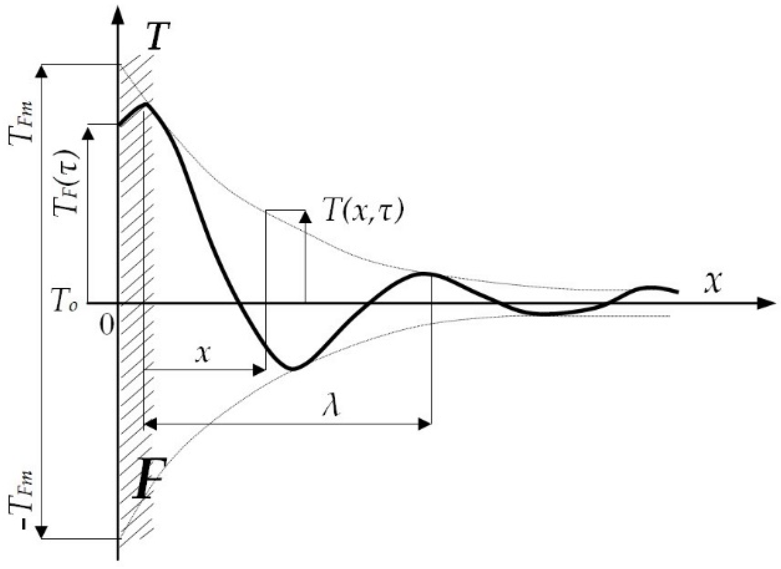
A semi-infinite body with initial temperature T_o, without internal heat sources, subjected to a temperature forcing on the external surface F according to the cosine function: ΔT = (T_m − T_o)∙cos(ω + τ).

At small penetration depths of periodic temperature changes, the issue can be considered as one-dimensional heat conduction in a flat semi-infinite body [47]:

$$T\left(x,\tau \right)=T_o+\left(T_m-T_o\right)\cdot exp\left(-\sqrt{\frac{\omega }{2a}}x\right)\cdot cos\left(\omega \cdot \tau -\sqrt{\frac{\omega }{2a}}x\right)$$

(10)

It can be noted that, inside a semi-infinite body, the temperature also changes according to the cosine function with an appropriately reduced amplitude and phase shift—Figure 1. The amplitude of temperature change T_xm at a distance x from the external surface F of a semi-infinite body is determined from Equation (10) when:

$$cos\left(\omega \cdot \tau -\sqrt{\frac{\omega }{2a}}x\right)=1$$

(11)

That is, as you move away from the body surface, the ratio of the amplitude at depth x, to the amplitude at the body surface F (i.e., when x = 0) decreases exponentially according to the formula:

$$\frac{T_{xm}}{T_{Fm}}=exp\left(-\sqrt{\frac{\omega }{2a}}x\right)$$

(12)

The phase shift increases with increasing frequency and is also dependent on the structure of the body material. The graph of the temperature change is contained between the dashed lines ±T_Fm (Figure 1), which approach each other as the distance x from the external surface F increases. From an application point of view, an important parameter is the effective penetration depth of the temperature wave. The penetration depth of a temperature wave can be defined as the distance over which the wave amplitude decreases 100 times, i.e.,

$$x=\sqrt{\frac{2\cdot a}{\omega }}\cdot ln\left(\frac{T_{Fm}}{T_{xm}}\right)=\sqrt{\frac{2\cdot a}{\omega }}\cdot ln(100)=6.51\cdot \sqrt{\frac{a}{\omega }}$$

(13)

Assuming an e-time change, which is a typical assumption valid in active thermography, then:

$$x=\sqrt{\frac{2\cdot a}{\omega }}\cdot lne=\sqrt{\frac{2\cdot a}{\omega }}$$

(14)

The penetration depth decreases with increasing forcing frequency of the temperature wave (T_m − T_o)∙cos(ω + τ) and depends on the diffusivity a, i.e., on the thermal parameters λ, ρ, c_p of the body. Knowing its approximate thickness and using the formulas given above, it is possible to choose the appropriate forcing frequency. It is worth noting that the temperature wavelength does not change as one moves deeper into the body, as it does not depend on x.

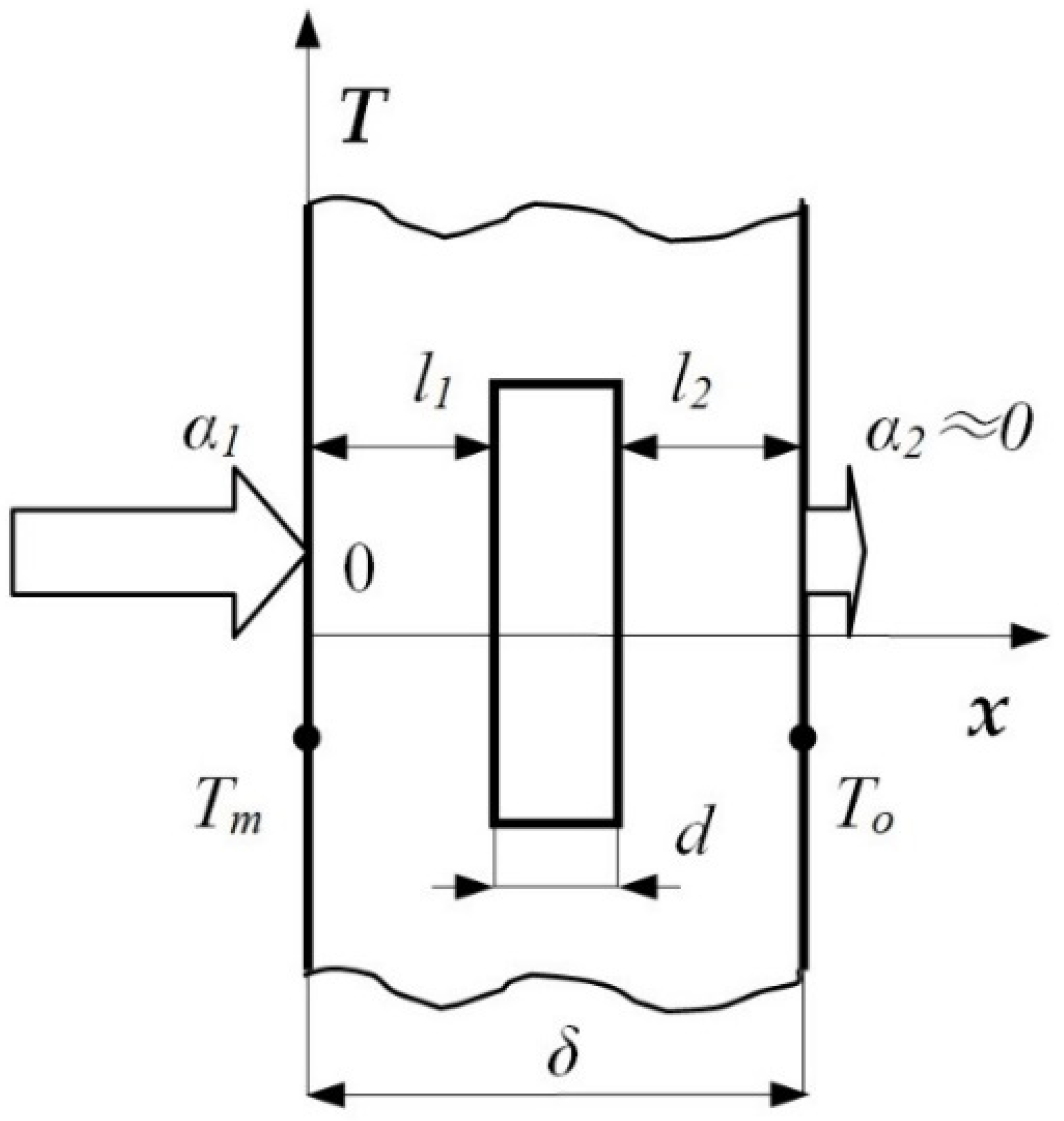
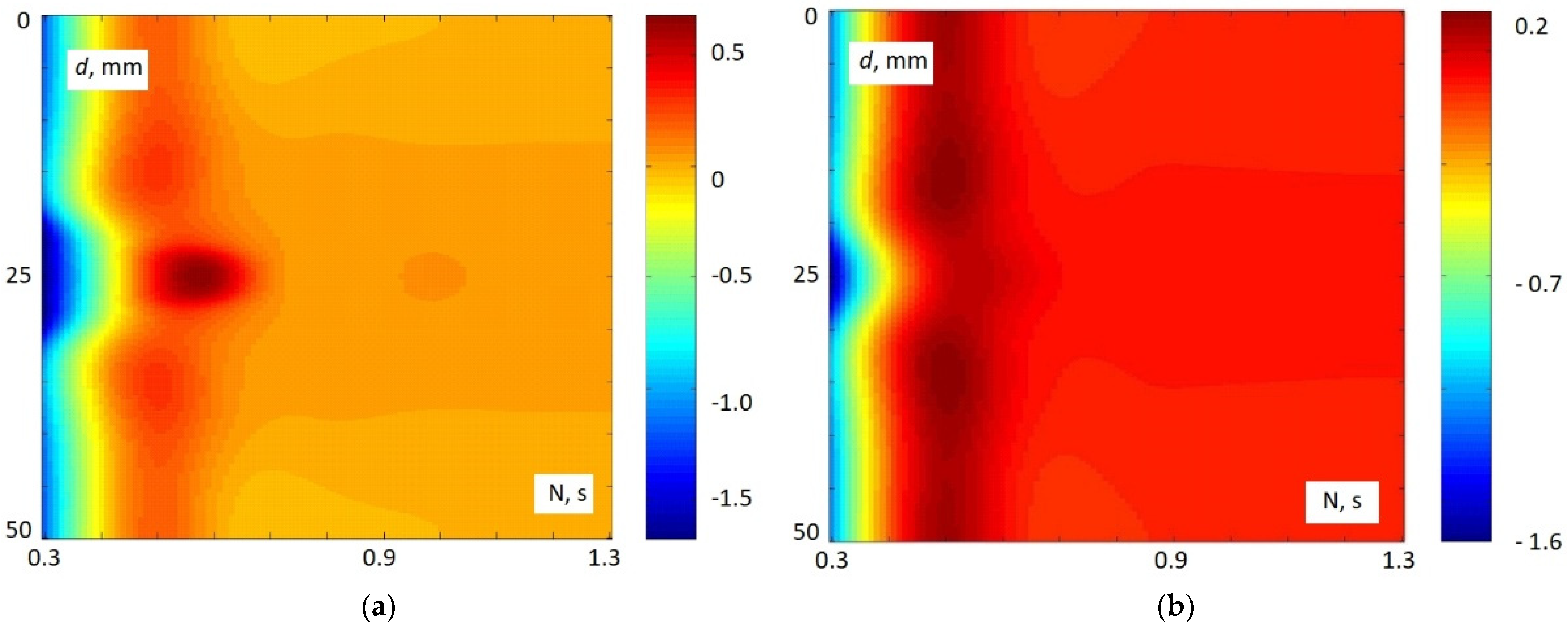
Example of Application of the Theoretical Model—Defective Material

It concerns the process of heating an unlimited plate of thickness δ with an extensive, internal defect of thickness d, located at a depth l₁ from the surface of the plate (Figure 2). It is assumed in the task that the thermal conductivity coefficient in the area of the defect takes the value close to zero: λ_def ≈ 0. Consequently, the heat transfer coefficient on the opposite side to the heated one will also assume the value to be close to zero: α₂ ≈ 0. The above example may serve as a method for locating air gaps in the thermal insulation of a building [44,45].

The time course of the temperature on the other side of the plate without defect, under the above assumptions (x = δ, i.e., in Formula (9) x/δ = 1), follows the formula:

$$T\left(x=\delta ,\tau \right)=T_o+\left(T_m-T_o\right)\left[1-{{\displaystyle \sum }}_{n=1}^{\infty }\frac{2sin{\mu }_n}{{\mu }_n+cos{\mu }_{n}sin{\mu }_n}cos{\mu }_n\cdot exp\left(-{\mu }_n^2\frac{a\cdot \tau }{{\delta }^2}\right)\right],$$

(15)

where: ${\mu }_n=\frac{{\alpha }_2\cdot \delta }{\lambda }ctg{\mu }_n$.

If there is a defect (α₂→0), the heating of the plate follows according to the Formula (16):

$$T\left(x=\delta ,\tau \right)=T_o+\left(T_m-T_o\right)\left[1-{\displaystyle \sum }_{n=1}^{\infty }\frac{2sin{\mu }_n}{{\mu }_n+cos{\mu }_{n}sin{\mu }_n}\cdot exp\left(-{\mu }_n^2\frac{a\cdot \tau }{l_1^2}\right)\right],$$

(16)

where: ${\mu }_n=\frac{{\alpha }_2\cdot l_1}{\lambda }ctg{\mu }_n$.

From the subtraction of Formulas (15) and (16), it is possible to determine the temperature difference ΔT(x, τ) for two cases of heating of the plate, i.e., absence of the defect and its occurrence. However, the problem is complex as it requires determination of several elements of μ_n of the transcendental equation, five of which are presented in Table 1.

The procedure of determining the accuracy of determining the depth of these defects is described in papers [39,48,49].

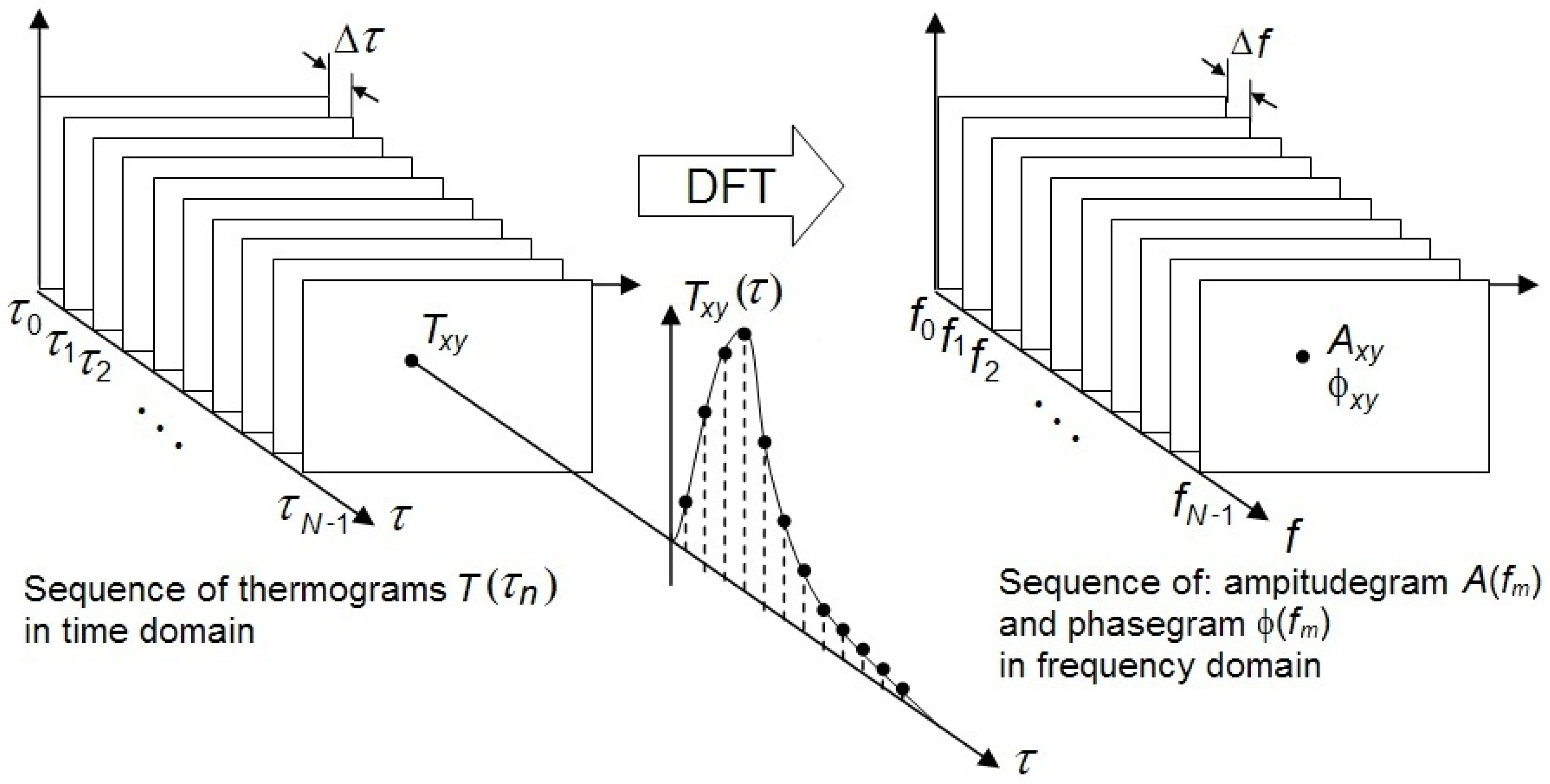
3. Pulsed Thermography (PT) and Pulsed Phase Thermography (PPT)

In the field of non-destructive testing, there is a concept called pulse thermography (PT). This term is used to describe active techniques for non-destructive diagnostics of materials in which the test sample (semi-infinite body) is subjected to a pulsed thermal forcing on a surface of a given duration. The forcing can also be a series of pulses.

The essence of pulse thermography is explained in Figure 3. Infrared radiation emitted by an excitation radiation source 3 (e.g.,: infrared radiator, high-power bulb, flash lamp, laser) falls on the tested object 1, which heats up. At the same time, it emits infrared radiation, which is recorded by the thermal imaging camera 2. The intensity of the radiation from object 1 depends on the type of material the object is made of and on discontinuities or defects present in it.

After switching off the source of excitation radiation, the object cools down to the ambient temperature. It can be seen in the thermograms that the object does not cool uniformly over its entire surface. Some areas cool faster than others. Thermograms are stored in the memory of computer 5. The system switching the source of infrared radiation is the triggering system 4. It is controlled by computer 5, which simultaneously records a sequence of thermograms coming from the camera. On the basis of the registered sequence of n thermograms, it is possible to determine the time course of the temperature T(n) for a given pixel. In order to do that, the procedures of matching thermograms in a series must first be applied so that the pixels of the thermogram correspond to the same point on the surface of the tested object. In case the object is moving, thermograms synchronised with the movement of the test object shall be recorded.

In the PT method, it is very important to correctly select the source of thermal energy supplied to the object. It can be a flash lamp, an infrared illuminator, a laser beam, an air or water thermal flux. The parameters of standard energy sources are listed in

Table 3. Overview of thermal energy sources used in pulsed thermography.

Energy Source	Power	Pulse Time	Notes
Flash lamp	10 kJ	5 ÷ 50 ms	Small size of the heating surface: 0.3 m × 0.3 m
Quartz lamp	>10 kW	1 ÷ 15 s	Slow heating
Lamp with carbon fibre	>2 kW	÷5 s	Slow heating
Heater	250 W ÷ 5 kW	>60 s	Very slow heating
Cold water, hot water	>1 kW	>60 s	Low efficiency
Air: warm, cold	>1 kW	>1 s	Low efficiency
Ruby laser	order GW	10 ÷ 30 ns	Uniformity over a small area
Pulse laser	order GW	10 ÷ 100 ns	Uniformity over a small area
High frequency	Order MW ÷ GW	some ms	Heat generated by friction of molecules
Ultrasound	>1 kW	some ms	Conversion of kinetic energyto the internal energy

. The pulse duration: ns (μs) ÷ s depends on the thickness and thermal parameters of the tested material. The penetration depth of thermal waves can be determined using Formulas (13) and (14).

Introducing the term R makes it possible to estimate an equation for a system of two bodies, i.e., the material inspected and the material of the defect as a second layer [50]:

$$T\left(x=0,\tau \right)=T_0+\frac{C_{IH}}{\sqrt{\tau }}\left\{1+2{\displaystyle \sum }_{n=1}^{\infty }{\left(-R\right)}^n\left[exp\left(-\frac{n^2\cdot L^2}{a\cdot \tau }\right)\right]\right\}$$

(17)

where:

$$R=\frac{e_1-e_2}{e_1+e_2}$$

(18)

thermal reflectance; index 1 refers to the coating, index 2 to the substrate (background). $e=\sqrt{\lambda \cdot \rho \cdot c_p}$- heat effusivity coefficient, $\frac{\mathrm{W}\cdot {\mathrm{s}}^{1/2}}{{\mathrm{m}}^2\cdot \mathrm{K}}$.

The parameter C_IH depends on the properties of tested surface and power delivered by external source of energy. It must be mentioned that C_IH depends on the spatial power density, not just the power. Furthermore, the sum term in Equation (17) results from multiple reflection and is only significant in case of thermally thin layers, otherwise the first term dominates

For R = 0, there is no difference in terms of thermal properties of the materials. The greater the value of R, the better the chance of detecting a defect against the background of the material inspected. For instance, for R < 0, which is the case when e_mat > e_def, the defect is a thermal insulator with respect to the material of the first layer. Because of that, heat is accumulated in the first layer and the temperature on the surface rises faster than it would in a homogeneous, defect-free material. For R > 0, the defect receives heat from the first layer, causing the material to cool fast. These situations are depicted in Figure 4, on the assumption that the coefficient C_IM is of a unit value in all the cases mentioned above. The influence of R parameter of the decay ratio can also be observed. The value and sign of R indicate the degree and character of the thermal mismatch between the materials. By comparing experimental data with the reference curve registered for defect free case, we can estimate if a defect manifests its presence and if it is a thermal conductor or insulator with relation to tested material.

Another variant of PT pulse thermography is called pulse phase thermography (PPT). As a result of PPT thermography, a series of so-called amplitudograms (as in PT thermography) and phasograms (phase thermograms) are obtained. The possibility of processing in the time and frequency domain is given in Figure 5 after the work [51].

PPT thermography using Fourier transform shows some advantages over PT thermography, e.g., the quality of phase thermograms obtained with this method is less affected by the non-uniformity of heating of the tested surface. On the other hand, it is basically a qualitative method and attempts to obtain quantitative information from phasograms such as defect depth, and this does not yet give satisfactory results. This is due to the property of the Fourier transform, which suppresses all temporal information from which the depth of the structure under investigation can be determined. The wavelet transform (WT) used in PPT preserves the temporal information and therefore makes it possible to determine the defect depth below the surface.

In the work [52], among the various wavelets, it was shown that the best one would be the Morlet wavelet as the primal wavelet described by the formula:

$$h\left(\tau \right)=exp(-j{\omega }_0\tau )\cdot exp\left(-\frac{{\tau }^2}{2}\right)$$

(19)

where: $j=\sqrt{-1}$—imaginary unit.

The function (19) is the result of multiplying the Fourier basis function $exp(-j{\omega }_0\tau )$ by a Gauss window of variable size, defined by the so-called scale factor. The use of the Fourier basis function preserves the advantages of the Fourier transform. Figure 6 shows the real part (solid line) and the imaginary part (dashed line) of the Morlet wavelet.

The wavelet transform is the inverse Fourier transform of the product of H(ω) and F(ω). The Fourier transform of the Morlet wavelet is defined as follows:

$$\begin{gathered} H\left(\omega \right)=\sqrt{\frac{\pi }{2}}\left\{exp\left[-\frac{{(\omega -{\omega }_o)}^2}{2}\right]+exp\left[-\frac{{(\omega +{\omega }_o)}^2}{2}\right]\right\}+ \\ +j\sqrt{\frac{\pi }{2}}\left\{-exp\left[-\frac{{(\omega -{\omega }_o)}^2}{2}\right]-exp\left[-\frac{{(\omega +{\omega }_o)}^2}{2}\right]\right\}. \end{gathered}$$

(20)

This is a complex function that consists of two Gaussian functions shifted to +ω_o and −ω_o. The real part is even and symmetric about the origin of the coordinate system. The imaginary part is odd and also symmetric about the origin of the coordinate system (Figure 7).

In the work [53], simulations were carried out using the Morlet wavelet transform. For this purpose, a two-dimensional PT model was developed based on the finite difference method and the MATLAB toolbox ’Partial Differential Equations’ with this model, the classical parabolic differential equation of heat conduction (1) was solved. The simulations involved a model of heat conduction in a 5 mm thick aluminium plate with a 5 mm diameter hole drilled. The hole depth was assumed in the range of 0.4 ÷ 4.5 mm. It is known from classical PPT thermography that most of the energy of a heat pulse is contained in the low frequency range. Therefore, ω_o = 2 Hz was assumed in the simulations, which corresponds to a frequency of f = 0.32 Hz. Figure 8 shows the WT phases for defect depths d equal to 0.5 and 2.5 mm. Both defects are clearly visible.

For each case, the value of the so-called wavelet shift factor (translation) N was determined, for which it was possible to achieve the maximum contrast between the area of the plate with defect and the area without defect. The translation factor N is one of the parameters defining the derived wavelet, the so-called “daughter” wavelet. It defines the shift of the wavelet on the time axis, which is expressed in seconds. The second parameter defining the derived wavelet is the so-called scale factor. Figure 9 shows the dependence of the value of the wavelet shift factor N as a function of the defect depth d. A linear relationship between these parameters can be observed—the line of maximum contrast is marked. By preserving the time information, the WT transformation also preserves the depth information.

Figure 10 shows the results of an experimental study of the location of a defect (circular inclusion) in a carbon fibre reinforced plastic plate. The plate was heated by two flash lamps with a power of 6.4 kJ/10 ms. A thermal imaging camera recorded 100 thermograms at 0.07 to 7.07 s after the flash at an interval of 0.07 s. The WT experimental study assumed a wavelet shift factor of N = 0.77 s and ω_o = 2 Hz. In Figure 10, the presence of the inclusion can be clearly observed.

The described method belongs to the group of PPT type methods. The phase-grams obtained as a result of its application result from the existence of the wavelet shift factor N and the so-called scale factor not discussed here. Examples of the use of the wavelet transform in active thermography are described in numerous works, e.g., [43,54,55].

A kind of pulse thermography, sometimes distinguished as a separate type of thermography, is long-pulse thermography, in which a response to a constant thermal forcing during the heating phase (so-called step-heating) or cooling phase is observed [56,57]. Due to the ease of providing such forcing, it is readily used. Knowing the time response to step heating facilitates the determination of the defect depth and its thermal character, i.e., we check whether it is a conductor or insulator in relation to the properties of the tested material.

The relevant formula for the time response to step excitation can be quoted after [50]:

$$T\left(x=0,\tau \right)=T_0+C_{SH}\sqrt{\tau }\left\{1+2{\displaystyle \sum }_{n=1}^{\infty }{\left(-R\right)}^n\left[exp\left(-\frac{n^2\cdot L^2}{a\cdot \tau }\right)-\frac{n\cdot L\sqrt{\pi }}{\sqrt{a\cdot \tau }}erfc\left(\frac{n\cdot L}{\sqrt{a\cdot \tau }}\right)\right]\right\}.$$

(21)

The parameter C_SH depends, as previously, on a number of factors, i.e., emissivity of the sample surface, reflection factor of material surface, irradiation intensity. In paper [56], the optimal time duration of step heating for above analytical model was discussed. Its applicability was examined by comparing temperature rises in time of the material with hidden subsurface defect with that obtained for a 3D numerical model created in the COMSOL software.

Formally, Equation (21) is an integral over the time of the pulse response represented as (17). Below, for illustrative purposes, an inverse operation is presented, i.e., a derivative of Equation (17), equivalent to (21). The equivalent symbol grouping some others k = n·L/a and:

$$S\left[x\right]=2{\displaystyle \sum }_{n=1}^{\infty }{\left(-\Gamma \right)}^n\left[x\right]$$

(22)

are introduced and the properties of the function of error and its derivative are deployed

$$erfc\left(x\right)=1-erf\left(x\right),$$

(23)

$$\frac{derfc\left(x\right)}{dx}=-\frac{2}{\sqrt{\pi }}exp(-x^2),$$

(24)

This yields the following:

$$\begin{array}{l}\frac{d\mathsf{\Delta }T}{dt}=\frac{C_{SH}}{2\sqrt{t}}\left\{1+S\left[exp\left(-\frac{k^2}{t}\right)-\frac{k\sqrt{\pi }}{\sqrt{t}}erfc\left(\frac{k}{\sqrt{t}}\right)\right]\right\}+\\ +C_{SH}\sqrt{t}\cdot S\left[-\frac{k^2}{t^2}exp\left(-\frac{k^2}{t}\right)+\frac{k\sqrt{\pi }}{2t\sqrt{t}}erfc\left(\frac{k}{\sqrt{t}}\right)-\frac{k\sqrt{\pi }}{\sqrt{t}}\frac{2}{\sqrt{\pi }}\frac{k}{2t\sqrt{t}}exp\left(-\frac{k^2}{t}\right)\right]=\\ =\frac{C_{SH}}{2\sqrt{t}}\left\{1+S\left[exp\left(-\frac{k^2}{t}\right)\right]\right\}-\frac{C_{SH}}{2}S\left[\frac{k\sqrt{\pi }}{t}erfc\left(\frac{k}{\sqrt{t}}\right)\right]+\\ +C_{SH}\cdot S\left[\frac{k^2}{t\sqrt{t}}exp\left(-\frac{k^2}{t}\right)+\frac{k\sqrt{\pi }}{2t}erfc\left(\frac{k}{\sqrt{t}}\right)-\frac{k^2}{t\sqrt{t}}exp\left(-\frac{k^2}{t}\right)\right]=\\ =\frac{C_{SH}}{2\sqrt{t}}\left\{1+S\left[exp\left(-\frac{k^2}{t}\right)\right]\right\}.\end{array}$$

(25)

We obtain the same equation as shown in (17), going back to the original symbols.

4. Lock-In Thermography (Modulated Thermography, Phase Sensitive Modulated Thermography)

In the field of non-destructive testing, there is the concept of so-called synchronous lock-in thermography, variations of which are also called modulated thermography, phase sensitive modulated thermography or heat wave thermography. This term is used to describe active techniques for non-destructive diagnostics of materials, in which the tested sample (semi-infinite body) is subjected to a harmonic thermal forcing on a surface with frequency ω. The analysis of the amplitude A and the phase shift angle φ of the rest with respect to the thermal forcing allows to determine the location and type of anomaly occurring in the tested body [58,59].

Assuming forcing on the surface of a semi-infinite body by a heat flux of density:

$$q=I_o\cdot exp(j\omega \tau ),$$

(26)

and amplitude I_o(x = 0), the response of a homogeneous object of the form is obtained:

$$T\left(x,\tau \right)=\frac{I_o}{\lambda }\sqrt{\frac{a}{j\omega }}\cdot exp\left(-x\sqrt{\frac{j\omega }{a}}\right)\cdot exp\left(j\omega \tau \right)$$

(27)

It may be noted that Equation (27) describes a heat wave, strongly damped along the x-axis.

For a semi-infinite body of thickness δ (e.g., a flat plate), consisting of two layers: a shell and a test body (substrate). The following formula for the temperature distribution on the surface of the shell is obtained:

$$T\left(x=0,\tau \right)=\frac{\left(1-R\right)I_o}{\lambda }\sqrt{\frac{a}{j\omega }}\cdot \left[\frac{1+R\cdot exp\left(-2\delta \sqrt{\frac{j\omega }{a}}\right)}{1-R\cdot exp\left(-2\delta \sqrt{\frac{j\omega }{a}}\right)}\right]\cdot exp(j\omega \tau )$$

(28)

The heat wave generated at the coating surface propagates to the inside of the test body, where it is partially reflected towards the coating. The occurrence of a defect at the interface between two layers (e.g., in the form of their cleavage) causes a local change of the R factor, which results in a change of the phase φ of the signal reflected from the surface of the coating. The penetration depth of the thermal wave x, similarly to the case (10), is described by the previously given Formula (14).

Inserting into Formula (14) $\omega =2\cdot \pi \cdot f$, it can be observed that the lower the frequency f of change of the thermal wave is, the greater the depth of penetration of this wave into the object x, i.e., if f₁ < f₂ then x₁ > x₂. This will result in a higher temperature at the surface of the test object, i.e., T₁ > T₂.

The time response to a cyclic heat excitation is expressed by the relation [50].

$$\begin{gathered} T\left(x=0, \tau \right)=\frac{1}{2}T\left(x=0,\omega \right)\cdot \left(1+\omega \tau \right), \\ T\left(x=0,\omega \right)=C_{PM}\left\{1+2{{\displaystyle \sum }}_{n=1}^{\infty }{\left(-R\right)}^n\left[exp\left(-2n\sigma L\right)\right]\right\}, \end{gathered}$$

(29)

where:

$$\sigma =\left(1+j\right)\sqrt{\frac{\omega }{2a}}$$

(30)

is a complex thermal wave number, m⁻¹.

The term C_PM is a function of intensity of the light modulated with frequency ω, optical reflectivity and σ parameter.

The literature [52] provides several types of lock-in synchronous thermography, they are:

• standard lock-in method,
• 4—bucket method,
• variance method,
• least squares method,
• flash method.

The implementation of the lock-in system along with the analysis of various technical aspects is discussed in depth in the book [60]. Entries [61,62,63] are some selected examples of applications of the lock-in technique in various branches of technology.

Lock-in thermography using ultrasound is also of great importance in practice. This type of thermography is characterised by shorter measurement time and better repeatability of measurements as compared to classical lock-in thermography. It is well suited to detecting cracks due to defect selective heating. Unfortunately, the necessity of direct contact as well as hiding the surface are clear drawbacks in comparison to optical heating methods.

The research development tendencies consist in the development of effective methods for the detection of smaller and smaller discontinuities and obtaining richer information on the investigated object. Difficulties are with ensuring the accepted accuracy of determining the dimensions of defects, i.e., lateral size and depth (the thickens of first layer). It is obtained by means of various data processing techniques used so far in other branches of technology combined with an analytical or numerical model of physical phenomena described in Section 2 of this paper. A list of representative bibliography on this subject can be found in papers [64,65,66,67].

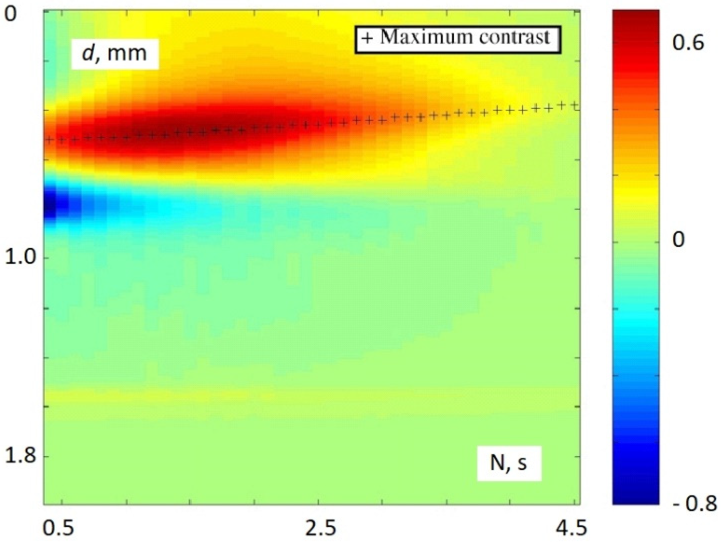
5. Example of Using Step Heating Response for Estimation of Defect Properties

In this section, the own crafted software called ‘IR defect detector v2022′ will be discussed as a practical effect of many research conducted by authors evaluating methods of material subsurface flaw detection and estimation of it properties. It is a fusion of various data processing techniques delivering semiautomatic detecting, counting and reporting of defects by analysis of single thermograms or thermograms sequence. Furthermore, it is possible to determine defects’ lateral size, depth at which they are located and thermal properties as compared to those of the material inspected. The program was created in the MATLAB environment. It provides a simple and intuitive GUI and implements various data processing techniques, i.e., contrast improving, 3D presentation, binarization, defects automatic labelling and what is the most important issue, one-dimensional analytical model of step heating response. The latter is needed for a depth evaluation as well as an Equation (21) was applied in code as an example of using the ‘piece of theory in practice’.

Its basic features are concentrated on the presentation of the thermograms and associated measurement data. They are as follows:

-

Uploading single thermogram or sequence from MATLAB file,

-

2D or 3D view of thermogram,

-

Displaying and input the time interval between two consecutive thermograms,

-

Displaying the geometrical resolution,

-

Raw and processed thermogram by applying contrast improvement or binarization,

-

Region of interest,

-

Colormaps,

-

Local or global thresholding for defect separation from the background,

-

Morphology operation for noise reducing and contrast improvement [24].

The programme has the following valuable functionalities achieved thanks to the filtered contrast FC/RIFC technique described in [68], providing its idea and technical details of implementation as 1D or 2D Gaussian smoothing filters. The algorithm of defect detection and its parameter assessment was discussed in detail in paper [69]:

-

Insensitivity to the nonuniform surface irradiation,

-

Automatic counting and reporting detected defects,

-

Defect lateral size estimation according to Otsu binarization with global thresholding [70];

-

Coordinates x,y of the central point of any detected defects;

-

Profile of defect depth according to the method given in [56] based on analysis of thermal response in time domain given by Equation (21);

-

Sign of the thermal mismatch factor R delivering the information if the flaw is thermal isolator or conductor—Equation (18).

Skipping some details, the processing steps leading to defect detection and characterization can be summarized as follows:

-

Record a reference thermogram,

-

Determine the reference temperature as an arithmetic mean from the reference thermogram,

-

Assume input values of 1D model, i.e., thermal mismatch parameter R, thermal diffusivity of tested material and required RIFC level,

-

Assume heating time (also end of recording),

-

Start thermal stimulation and record a thermogram sequence,

-

Apply relative incremental filtered contrast FC or RIFC (if depth determined) for all thermograms,

-

Detect and separate defective areas from the background on the basis of significant temperature differences by applying segmentation technique to the last thermogram,

-

Determine the coordinates x,y of characteristic points of defects (local maximum),

-

Find the sign of Γ for each defect in the point x,y on the basis of the sign of RIFC for the last recorded thermogram,

-

Estimate the lateral defect dimensions, i.e., minor and major axes,

-

Determine the depth of each defect for the coordinates x,y of the defect only or all pixels belonging to defective area (option),

-

The heating and data recording can be stopped earlier if:

-

RIFC in characteristic points of each defect reaches the assumed threshold of normalised temperature,

-

The surface temperature exceeds 90% of the material permissible temperature (it must be done manually).

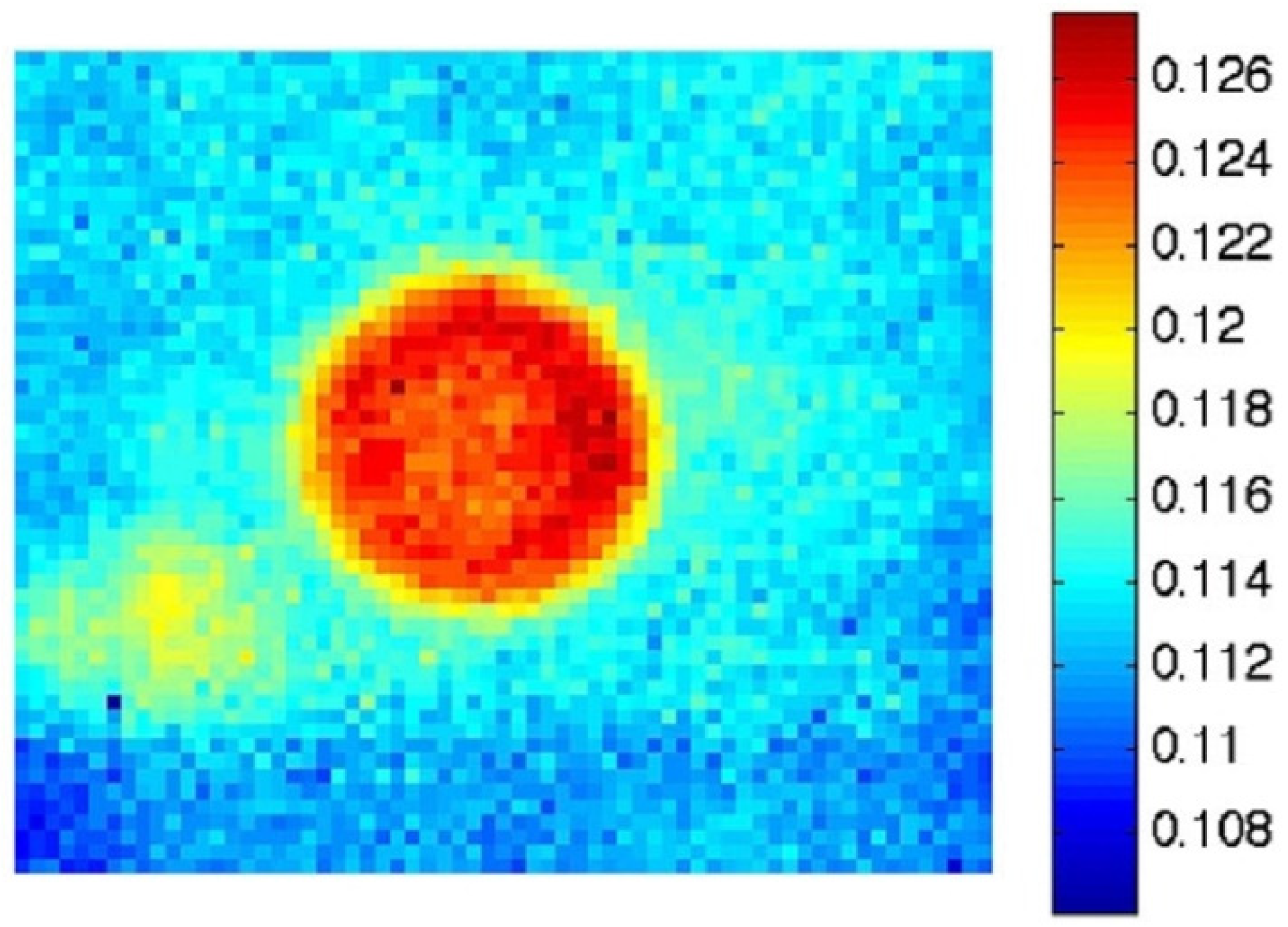
Example of Using the IR Defect Detector for PMMA Material Testing

A sample made out of a rectangular slab of PMMA with properties close to typical materials tested by thermographic NDT, e.g., composites and multi-layered laminates. From the bottom side of it, the holes of various diameters at various depths were drilled to emulate the occurrence of defects. The front part of defects was levelled with a milling cutter so that a flat surface was obtained. Due to this, defects had the shape of a cylinder with an open base and were filled with air. The front surface observed by IR camera was coated with black matt paint to provide constant high emissivity. The two 800 W lamps were symmetrically placed on a right and left side of the tested slab working as heat excitation. Full constant power (1600 W totally) was delivered to the tested material by heating phase. The thermal images were collected by an infrared camera IRS336F-13-NDT (FPA detector, spatial resolution: 336 × 256 pixels, NETD < 50 mK) connected to PC computer (2) via GigE network card with GenICam protocol used for linking the camera with PC and dedicated software that was primarily used to control excitation and export recorded data to MATLAB format.

In Figure 11a,b, we can see an example of thermogram (a) recorded at 40 sec. Two subsurface defected areas with bigger (on the left) and smaller (on the right) diameters revealed clearly. Applying so-called ‘filtered contrast FC’ or ‘relative incremental filtered contrast RIFC’ techniques of image smoothing, the effect of uneven heating is significantly compressed but some extra rings (locally lowering the processed signal value) occurred around the defective areas as an unnecessary artefact. It is better visible in a three-dimensional view, as shown in Figure 11b,d. If we look at Figure 11c,d, we see almost uniform background for defect-free areas. The estimated background from the original thermogram can be achieved by simple subtraction. For this objective, the smoothing filtering or morphology operations can be used. It is an idea of FC technique. Thanks to a slightly more complex RIFC method, instead of FC, the distribution of the processed thermal signal no longer depends on the C_SH coefficient, but only on the thermal mismatch R, thermal diffusivity a of the tested material and the depth of the defect L—Equation (21). If thickness of the tested material is much greater than thickness of the first layer above the defect the processed thermogram after RIFC technique is an estimation of so-called ‘normalized temperature’, i.e.,

$$RIFC\left(\tau \right)=2{\displaystyle \sum }_{n=1}^{\infty }{\left(-R\right)}^n\left[exp\left(-\frac{n^2\cdot L^2}{a\cdot \tau }\right)-\frac{n\cdot L\sqrt{\pi }}{\sqrt{a\cdot \tau }}erfc\left(\frac{n\cdot L}{\sqrt{a\cdot \tau }}\right)\right].$$

(31)

More discussion on these issues can be found in paper [68,69].

The lateral size of defect can be estimated on the basis of camera optical features and distance from camera to object given by the experimenter as a parameter of thermographic processing model. Because it is a possible source of error, it should be set as measured precisely [39]. For the standard lens 13 mm and pixel size 17 µm of IRS336F-13-NDT infrared camera, the horizontal and vertical resolutions corresponding to the field of view of a single pixel are IFOV = 17 µm/13 mm = 1 mrad. For instance, at a distance of 0.6 m, the effective field of view for single pixel expressed in mm is as follows: IFOV = IFOV_H = IFOV_V = 0.78 mm. The defects projected onto the material surface are shown in the lower left part of the Figure 12, presenting the GUI of the ‘IR defect detector’ software as well. It is an effect of image binarization into two classes: defective and defective-free (sometimes named also sound) areas. The known true dimensions can be compared with those evaluated by the used programme and are marked in the lower right corner of the Figure 12. The relative error of lateral size is about 12% for both defects. More precise measurements are possible and require use of the ‘size calibration factor’ also implemented in code.

As a result of our previous work, we confirmed the Vavilov [71] observation that the defect boundary (change of medium) corresponds to inflection point of temperature profile along the frontal surface observed by IR camera. Furthermore, the result of Otsu image binarization method (classified pixels as background or object) applied to local area near the defect instead of all pixels of thermal image estimates the boundary of defect correctly. It was confirmed by 3D numerical modelling, but some real experiments showed that accuracy of this method for flat located defects is generally not very high and c.a. 15–20%, but it is fast and easy to implement. This simple binarization can be used to estimate the inflection point instead of checking first or second derivatives of temperature profile. The derivatives are sensitive to the measurement noises and undesirable effect of noise amplification can be seen. This causes that precise detection of inflection point is not trivial and also error-prone.

The defect depth is evaluated by matching the relative incremental filtered RIFC curve versus time (please look at upper left part of Figure 12) to the analytical Equation (31) with some assumption on character of expected defects (here air holes) and thermal diffusivity of tested material as included in the equation—visible in the right panel named ‘Defect characterization’. The detailed explanation as to how the depth estimation works confirmed by simulations for analytical 1D model of thermal behaviour can be found in paper [56]. The true values of depths can be compared again with those evaluated for central points of defective areas and are marked in the lower right corner, as previously. This time the relative error is about 17% for both defects. There are some limitations influencing the accuracy of depth estimation. The most important is lateral heat diffusion that can be partially reduced if the defect features lateral size > depth and the R value is pre-estimated as input to the model—visible in Figure 12 often on a priori knowledge on expected kind of defect and thermal properties of the tested material. It is a general drawback of the method using an analytical equation as applied in created software. The higher the R uncertainty is, the higher depth uncertainty, too. In paper [69], there was discussed the influence of this R parameter of the smoothing filter, required for filtered contrast implementation, thermal parameters of the tested material and defect on expanded uncertainty of determination of defect depth. The Monte Carlo method was applied for the propagation of uncertainty distributions.

More precise measurements are possible, too, and require using the ‘depth calibration factor’. The sign of thermal mismatch discussed in previous sections is also estimated classifying each object as thermal insulator or conductor in relation to properties of known tested material. In both cases, defects (air holes) were correctly classified as ‘insulator’—the table with results visible appears in Figure 12.

In Figure 13, the result of flat defects surface estimation is presented. The one-dimensional model of thermal response given by Equation (21) was applied and repeated for every pixel belonging to defective area from Figure 12. Some imperfections of profile are visible close to the boundary of defect and slab caused by complex heat transfer conditions. Generally, it can be observed that the significant flatness of profile complied with expectations.

6. Conclusions

The selected part of theory was incorporated into the created software to provide the qualitative and quantitative assessment of materials and objects. The software was intensively tested with various materials such as PMMA, expanded PVC foam, composite deck boards with various internal defects such as air holes, water and iron inclusions, and seems to be a promising, effective tool for defect detection and characterization. The efficiency of any method must be validated in conditions close to real situations and materials, not only flat bottom holes. Primarily, the method could be potentially applied to detect inner defects and the quantitative determination of coating thicknesses. Generally, it is aimed as the next stage of our research; however, so far, we are still looking for more accurate and robust techniques of data processing because the accuracy of presented method even for special case is quite limited as discussed in the above section. We can estimate that for harder conditions of experiments and more complex object structure will be even worse. If accuracy is satisfactory, one possible future work will be an attempt of standardization of testing procedure and data processing techniques assuring reliable results with small uncertainties. The procedure of testing must fully comply with ASTM E1316-22 terminology and will be modelled on well-recognized and accepted standard ASTM E2582-21 used for testing composite panels and repair patches using flash thermography and other good practices.

References

1. Aastroem, T. From fifteen to two hundred NDT- methods in fifty years. In Proceedings of the 17th World Conference on Nondestructive Testing, Shanghai, China, 25–28 October 2008. [Google Scholar]
2. Aastroem, T. One hundred and one NDT- and machine diagnostic methods for the prevention of losses in critical machinery. In Proceedings of the 16th World Conference on NDT, Montreal, QC, Canada, 30 August–3 September 2004. [Google Scholar]
3. Farley, M. 40 years of progress in NDT—History as a guide to the future. In AIP Conference Proceedings; AIP Publishing LLC.: Melville, NY, USA, 2014; Volume 1581, p. 5. [Google Scholar] [CrossRef]
4. McCann, D.M.; Forde, M.C. Review of NDT methods in the assessment of concrete and masonry structures. NDTE Int. 2001, 34, 71–84. [Google Scholar] [CrossRef]
5. Johnson, G. Ultrasonic flaw detectors … and beyond: A history of the discovery of the tools of nondestructive technology. Quality 2013, 52, 22–25. [Google Scholar]
6. Greissel, M. Toward a safe return to flight. Quality 2004, 43, A10. [Google Scholar]
7. Bracciali, A. Railway Wheelsets: History, Research and Developments. Int. J. Railw. Technol. 2016, 5, 23–52. [Google Scholar] [CrossRef]
8. Zhu, K.Y.; Tian, G.Y.; Lu, R.S.; Zhang, H. A Review of Optical NDT Technologies. Sensors 2011, 11, 7773–7798. [Google Scholar] [CrossRef] [Green Version]
9. Available online: https://asnt.org/MajorSiteSections/About/Introduction_to_Nondestructive_Testing.aspx (accessed on 23 June 2022).
10. Marin, J.-Y.; Tretout, H. Advanced technology and processing tools for corrosion detection by infrared thermography. In Proceedings of the 5th AITA—International Workshop on Advanced Infrared Technology and Applications, Venice, Italy, 29–30 September 1999; pp. 128–133. [Google Scholar]
11. Doshvarpassand, S.; Wu, C.; Wang, X. An overview of corrosion defect characterization using active infrared thermography. Infrared Phys. Technol. 2019, 96, 366–389. [Google Scholar] [CrossRef]
12. Dorafshan, S.; Maguire, M.; Collins, W. Infrared Thermography for Weld Inspection: Feasibility and Application. Infrastructures 2018, 3, 45. [Google Scholar] [CrossRef] [Green Version]
13. Yao, Y.; Sfarra, S. Active thermography testing and data analysis for the state of conservation of panel paintings. Int. J. Therm. Sci. 2018, 126, 143–151. [Google Scholar] [CrossRef]
14. Theodorakeas, P.; Cheilakou, E.; Ftikou, E.; Koui, M. Passive and active infrared thermography: An overview of applications for the inspection of mosaic structures. J. Phys. Conf. Ser. 2015, 655, 012061. [Google Scholar] [CrossRef]
15. Kordatos, E.; Exarchos, D.; Stavrakos, C.; Moropoulou, A.; Matikas, T. Infrared thermographic inspection of murals and characterization of degradation in historic monuments. Constr. Build. Mater. 2013, 48, 1261–1265. [Google Scholar] [CrossRef]
16. Meola, C. Infrared thermography of masonry structures. Infrared Phys. Technol. 2007, 49, 228–233. [Google Scholar] [CrossRef]
17. Ibarra-Castanedo, C.; Piau, J.M.; Guilbert, S.; Avdelidis, N.P.; Genest, M.; Bendada, A.; Maldague, X.P.V. Comparative Study of Active Thermography Techniques for the Nondestructive Evaluation of Honeycomb Structures. Res. Nondestruct. Eval. 2009, 20, 1–31. [Google Scholar] [CrossRef]
18. Marani, R.; Palumbo, D.; Attolico, M.; Bono, G.; Galietti, U.; D’Orazio, T. Improved Deep Learning for Defect Segmentation in Composite Laminates Inspected by Lock-in Thermography 2021. In Proceedings of the IEEE 8th International Workshop on Metrology for AeroSpace (MetroAeroSpace), Naples, Italy, 23–25 June 2021; pp. 226–231. [Google Scholar] [CrossRef]
19. Osornio-Rios, R.A.; Antonio-Daviu, J.A.; De Jesus Romero-Trancoso, R. Recent industrial applications of infrared thermography: A review. IEEE Trans. Ind. Inform. 2018, 15, 615–625. [Google Scholar] [CrossRef]
20. Deane, S.; Avdelidis, N.P.; Ibarra-Castanedo, C.; Zhang, H.; Nezhad, H.Y.; Williamson, A.A.; Mackley, T.; Davis, M.J.; Maldague, X.; Tsourdos, A. Application of NDT thermographic imaging of aerospace structures. Infrared Phys. Technol. 2019, 97, 456–466. [Google Scholar] [CrossRef] [Green Version]
21. Tejedor, B.; Lucchi, E.; Bienvenido-Huertas, D.; Nardi, I. Non-destructive techniques (NDT) for the diagnosis of heritage buildings: Traditional procedures and futures perspectives. Energy Build. 2022, 263, 112029. [Google Scholar] [CrossRef]
22. Balaras, C.A.; Argiriou, A.A. Infrared thermography for building diagnostics. Energy Build. 2002, 37, 171–183. [Google Scholar] [CrossRef]
23. Kirimtat, A.; Krejcar, O. A review of infrared thermography for the investigation of building envelopes: Advances and prospects. Energy Build. 2018, 176, 390–406. [Google Scholar] [CrossRef]
24. Gryś, S.; Dudzik, S. Investigation on dual-domain data processing algorithm used in thermal non-destructive evaluation. Quant. Infrared Thermogr. J. 2020, 19, 196–219. [Google Scholar] [CrossRef]
25. Heifetz, A.; Shribak, D.; Zhang, X.; Saniie, J.; Fisher, Z.L.; Liu, T.; Sun, J.G.; Elmer, T.; Bakhtiari, S.; Cleary, W. Thermal tomography 3D imaging of additively manufactured metallic structures. AIP Adv. 2020, 10, 105318. [Google Scholar] [CrossRef]
26. Nowakowski, A.Z. Problems of Active Dynamic Thermography Measurement Standardization in Medicine. Pomiary Autom. Robot. Eng. Meas. Autom. Robot. 2021, 25, 51–56. [Google Scholar] [CrossRef]
27. Toivanen, J.M.; Tarvainena, T.; Huttunen, J.; Savolainen, T.; Orlande, H.; Kaipio, J.; Kolehmainen, V. 3D thermal tomography with experimental measurement data. Int. J. Heat Mass Transf. 2014, 78, 1126–1134. [Google Scholar] [CrossRef]
28. Koutsantonis, L.; Rapsomanikis, A.N.; Stiliaris, E.; Papanicolas, C.N. Examining an image reconstruction method in infrared emission tomography. Infrared Phys. Technol. 2019, 98, 266–277. [Google Scholar] [CrossRef] [Green Version]
29. Vallerand, S.; Darabi, A.; Maldaque, X. Defect detection in pulsed thermography: A comparison of Kohonen and perceptron neural networks. In Thermosense XXI; SPIE: Orlando, FL, USA, 1999; Volume 3700, pp. 20–25. [Google Scholar]
30. Dudzik, S. Two-stage neural algorithm for defect detection and characterization uses an active thermography. Infrared Phys. Technol. 2015, 71, 187–197. [Google Scholar] [CrossRef]
31. He, Y.; Deng, B.; Wang, H.; Cheng, L.; Zhou, K.; Cai, S.; Ciampa, F. Infrared machine vision and infrared thermography with deep learning: A review. Infrared Phys. Technol. 2021, 116, 103754. [Google Scholar] [CrossRef]
32. Cao, Y.; Dong, Y.; Cao, Y.; Yang, J.; Yang, M.Y. Two-stream convolutional neural network for non-destructive subsurface defect detection via similarity comparison of lock-in thermography signals. NDTE Int. 2020, 112, 102246. [Google Scholar] [CrossRef]
33. Marani, R.; Palumbo, D.; Galietti, U.; Stella, E.; D’Orazio, T. Automatic detection of subsurface defects in composite materials using thermography and unsupervised machine learning. In Proceedings of the 2016 IEEE 8th International Conference on Intelligent Systems (IS), Sofia, Bulgaria, 4–6 September 2016. [Google Scholar] [CrossRef]
34. Burleigh, D.D. A bibliography of non-destructive testing (NDT) of composite materials performed with infrared thermography and liquid crystals. In Proceedings of the SPIE 0780, Thermosense IX: Thermal Infrared Sensing for Diagnostics and Control, Orlando, FL, USA, 11 May 1987; pp. 250–255. [Google Scholar]
35. Bing Wang, S.Z.; Lee, T.-L.; Fancey, K.S.; Mi, J. Non-destructive testing and evaluation of composite materials/structures: A state-of-the-art review. Adv. Mech. Eng. 2014, 12, 1–28. [Google Scholar] [CrossRef] [Green Version]
36. Lucchi, E. Applications of the infrared thermography in the energy audit of buildings: A review. Renew. Sustain. Energy Rev. 2018, 82 Pt 3, 3077–3090. [Google Scholar] [CrossRef]
37. Milovanović, B.; Banjad Pečur, I. Review of Active IR Thermography for Detection and Characterization of Defects in Reinforced Concrete. J. Imaging 2016, 2, 11. [Google Scholar] [CrossRef]
38. Minkina, W.; Chudzik, S. Determination of thermal parameters of heat-insulating materials using artificial neural networks. Metrol. Meas. Syst. 2003, 10, 33–49. [Google Scholar]
39. Minkina, W.; Dudzik, S. Infrared Thermography—Errors and Uncertainties; John Wiley & Sons Ltd., Wiley—Blackwell: Chichester, UK, 2009; Available online: https://www.wiley.com/en-ie/Infrared+Thermography:+Errors+and+Uncertainties-p-9780470682241 (accessed on 23 June 2022).
40. Minkina, W. Theoretical Basics of Radiant Heat Transfer—Practical Examples of Calculation for the Infrared (IR) Used in Infrared Thermography Measurements. Quant. Infrared Thermogr. J. 2021, 18, 269–282. [Google Scholar] [CrossRef]
41. Bayazitoğlu, Y.; Özişik, M.N. Elements of Heat Transfer; McGraw-Hill Book Company: New York, NY, USA, 1988. [Google Scholar]
42. Janna, W.S. Engineering Heat Transfer; CRC Press: Washington, DC, USA, 2009. [Google Scholar]
43. Parrany, A.M. Damage detection in circular cylindrical shells using active thermography and 2-D discrete wavelet analysis. Thin-Walled Struc. 2019, 136, 34–49. [Google Scholar] [CrossRef]
44. Baвилoв, B.П. Teплoвыe мeтoды кoнтpoля cтpyктyp и издeлий paдиoэлeктpoники (Thermal Control Methods for Electronic Components and Systems); Paдиo и Cвязь (Radio and Communications): Moscow, Russia, 1984. [Google Scholar]
45. Baвилoв, B.П. Teплoвыe мeтoды нepaзpyшaющeгo кoнтpoля—Cпpaвoчник (Thermal Non-Destructive Testing Methods—Guide); Maшинocтpoeниe (Machine Maintenance): Moscow, Russia, 1991. [Google Scholar]
46. Hobler, T. Ruch Ciepła i Wymienniki (Eng. Heat Movement and Exchangers), 5th ed.; WNT: Warsaw, Poland, 1979. [Google Scholar]
47. Wiśniewski, S.; Wiśniewski, T.S. Wymiana Ciepła (Eng. Heat Exchange); WNT: Warsaw, Poland, 1997. [Google Scholar]
48. Minkina, W.; Dudzik, S. Simulation analysis of uncertainty of infrared camera measurement and processing path. Measurement 2006, 39, 758–763. [Google Scholar] [CrossRef]
49. Minkina, W.; Dudzik, S.; Gryś, S. Errors of thermographic measurements—exercises. In Proceedings of the 10th International Conference on Quantitative Infrared Thermography (QIRT’2010), Quebec City, QC, Canada, 27–30 July 2010. [Google Scholar] [CrossRef]
50. Osiander, R.; Maclachlan Spicer, J.W.; Murphy, J.C. Thermal nondestructive evaluation using microwave sources. Mater. Eval. 1995, 53, 942–948. [Google Scholar]
51. Baran, J. Analiza sekwencji termogramów w dziedzinie częstotliwości (Eng. Frequency domain thermogram sequence analysis). In Wybrane Problemy Współczesnej Termografii i Termometrii w Podczerwieni (Eng. Selected Problems of Contemporary Thermography and Infrared Thermometry); Minkina, W., Ed.; Publishing House of Częstochowa University of Technology: Częstochowa, Poland, 2011; pp. 79–98. [Google Scholar]
52. Maldague, X.P. Theory and Practice of Infrared Technology for Nondestructive Testing; John Wiley & Sons Int.: New York, NY, USA, 2001. [Google Scholar]
53. Galmiche, F.; Maldague, X. Wavelet transform applied to pulsed phased thermography. In Proceedings of the 5th AITA—International Workshop on Advanced Infrared Technology and Applications, Venice, Italy, 29–30 September 1999; Grinzato, E., Bison, P.G., Mazzoldi, A., Eds.; pp. 117–122. [Google Scholar]
54. Zauner, G.; Mayr, G.; Hendorfer, G. Application of wavelet analysis in active thermography for non-destructive testing of CFRP composites. In Proceedings of the Wavelet Applications in Industrial Processing IV, 63830E (2006), Optics East, Boston, MA, USA, 12 October 2006. [Google Scholar] [CrossRef]
55. Olbrycht, R.; Więcek, B.; Gralewicz, G.; Świątczak, T.; Owczarek, G. Comparison of Fourier and wavelet analyses for defect detection in lock-in and pulse phase thermography. Quant. InfraRed Tghermogr. J. 2007, 4, 219–232. [Google Scholar] [CrossRef]
56. Gryś, S.; Minkina, W.; Vokorokos, L. Automated characterisation of subsurface defects by active IR thermographic testing—Discussion of step heating duration and defect depth determination. Infrared Phys. Technol. 2015, 68, 84–91. [Google Scholar] [CrossRef]
57. Palumbo, D.; Cavallo, P.; Galietti, U. An investigation of the stepped thermography technique for defects evaluation in GFRP materials. NDTE Int. 2019, 102, 254–263. [Google Scholar] [CrossRef]
58. Troitsky, O. Pulsed thermal nondestructive testing of layered materials. In Proceedings of the SPIE, 1933, Thermosense XV, An International Conference on Thermal Sensing and Imaging Diagnostic Applications, Orlando, FL, USA, 6 April 1993; pp. 309–312. [Google Scholar]
59. Wu, D.; Salerno, A.; Schönbach, B.; Hallin, H.; Busse, G. Phase sensitive modulation thermography and its applications for NDE. In Proceedings of the SPIE, 3056, Thermosense XIX, An International Conference on Thermal Sensing and Imaging Diagnostic Applications, Orlando, FL, USA, 4 April 1997; pp. 176–183. [Google Scholar]
60. Breitenstein, O.; Warta, W.; Langenkamp, M. Lock in Thermography: Basics and Use for Evaluating Electronic Devices and Materials; Series: Springer Series in Advanced Microelectronics 10; Springer: Berlin/Heidelberg, Germany, 2010; pp. 61–72. [Google Scholar]
61. Qu, Z.; Jiang, P.; Zhang, W. Development and application of infrared thermography non-destructive testing techniques. Sensors 2020, 20, 3851. [Google Scholar] [CrossRef]
62. Zrhaiba, A.; Balouki, A.; Elhassnaoui, A.; Yadir, S.; Halloua, H.; Sahnoun, S. A simple method for determining a thickness of metal based on lock-in thermography. Surf. Rev. Lett. 2020, 27, 1930003. [Google Scholar] [CrossRef]
63. Kandeal, A.W.; Elkadeem, M.; Thakur, A.K.; Abdelaziz, G.B.; Sathyamurthy, R.; Kabeel, A.; Yang, N.; Sharshir, S.W. Infrared thermography-based condition monitoring of solar photovoltaic systems: A mini review of recent advances. Sol. Energy 2021, 223, 33–43. [Google Scholar] [CrossRef]
64. Dillenz, A.; Busse, G. Ultraschall Burst-Phasen-Thermografie. Mater. Test. 2001, 43, 30–34. [Google Scholar] [CrossRef]
65. Park, H.; Choi, M.; Park, J.; Kim, W. A study on detection of micro-cracks in the dissimilar metal weld through ultrasound infrared thermography. Infrared Phys. Technol. 2014, 62, 124–131. [Google Scholar] [CrossRef]
66. Umar, M.Z.; Vavilov, V.; Abdullah, H.; Ariffin, A.K. Ultrasonic infrared thermography in non-destructive testing: A review. Russ. J. Nondestruct. Test. 2016, 52, 212–219. [Google Scholar] [CrossRef]
67. Świderski, W. Comparison of image analysis methods on the example of ultrasonic thermography of an aramid composite. J. Kones 2019, 26, 145–150. [Google Scholar] [CrossRef] [Green Version]
68. Gryś, S. New thermal contrast definition for defect characterisation by active thermography. Measurement 2012, 45, 1885–1892. [Google Scholar] [CrossRef]
69. Gryś, S. Filtered thermal contrast based technique for testing of material by infrared thermography. Opto-Electron. Rev. 2011, 19, 234–241. [Google Scholar] [CrossRef] [Green Version]
70. Gryś, S.; Vokorokos, L.; Borowik, L. Size determination of subsurface defect by active thermography—Simulation research. Infrared Phys. Technol. 2014, 62, 147–153. [Google Scholar] [CrossRef]
71. Baвилoв, B.П.; Шиpяeв, B.B. Cпocoб oпpeдeлeниa paзмepoв дeφeктoв пpи тeплoвoм кoнтpoлe (Eng. The method for determining the size of defects during thermal control). Дeφeктocкoпия 1979, 11, 63–65. [Google Scholar]
Figure 1. Temperature change T(x, τ) in a semi-infinite body along the x-axis when changing the external surface temperature F according to the cosine function-case for a selected time instant τ.
Energies 15 04865 g001
Figure 2. Example of using the method of temperature forcing at the plate edge to locate a defect inside the plate—Formula (8).
Energies 15 04865 g002
Figure 3. Diagnostic setup using pulse thermography: 1—object under test, 2—thermovision camera, 3—source of thermal radiation, 4—triggering system, 5—microcomputer.
Energies 15 04865 g003
Figure 4. Temperature rise of the surface of a homogeneous material (R = 0) and of a material with a defect R ≠ 0 for a pulse excitation as in Equation (17).
Energies 15 04865 g004
Figure 5. Sequence of images in the time and frequency domains.
Energies 15 04865 g005
Figure 6. Morlet wavelet: solid line-real part, dashed line-imaginary part.
Energies 15 04865 g006
Figure 7. Fourier transform of a Morlet wavelet.
Energies 15 04865 g007
Figure 8. WT phase at defect depth: (a) 0.5 mm and (b) 2.5 mm. Reprinted and adapted with permission from Ref. [53]. Copyright 1999, AITA.
Energies 15 04865 g008
Figure 9. Wavelet shift factor N for which the defect location is best visible. Reprinted and adapted with permission from Ref. [53]. Copyright 1999, AITA.
Energies 15 04865 g009
Figure 10. Results of applying the WT transformation to a carbon fibre reinforced plastic panel with a circular inclusion defect. Reprinted with permission from Ref. [53]. Copyright 1999, AITA.
Energies 15 04865 g010
Figure 11. Example of 2D/3D thermogram no. 120 at 40 s. of heating phase: (a,b) measured temperature in °C, (c,d) processed one with relative incremental filtered contrast technique RIFC in dimensionless units.
Energies 15 04865 g011
Figure 12. Screenshot of ‘IR defect detector’ GUI with two defects detected and parametrized.
Energies 15 04865 g012
Figure 13. The result of estimated profile of two flat defects.
Energies 15 04865 g013