Numerical Study of the Effect of the Rolling Motion on the Subcooled Flow Boiling in the Subchannel

Abstract

The marine environment may change the force on the fluid and inevitably influence bubble behavior and the two-phase flow in the reactor core, which are vital to the safety margin of a nuclear reactor. To explore the effect of the marine motion on the flow and heat transfer features of subcooled flow boiling in the reactor core, the volume of fluid (VOF) method is employed to reveal the interaction between the interface structure and two-phase flow in the subchannel under rolling motion. The variations of several physical parameters are obtained, including the transverse flow, the vapor volume fraction, the vapor adhesion ratio, and the phase distribution of boiling two-phase flow with time. Sensitivity analyses of the amplitude and the period of the rolling motion were performed to demonstrate the mechanisms of the influence of the rolling motion. We found that the transverse flow in the subchannel was mainly affected by the Euler force under the rolling motion. In contrast to the two-phase flow in the static state, the vapor volume fraction and vapor adhesion ratio show different characteristics under rolling motion. Additionally, the onset of significant void (OSV) point changes periodically under rolling motion.

1. Introduction

An offshore floating nuclear plant combines a nuclear power plant and a floating platform. Its flexibility is a huge advantage in energy supply. However, marine conditions will change the force on the fluid and inevitably influence the two-phase flow, bubble behavior, and void fraction in the reactor core, which are vital to the occurrence of boiling crisis phenomena and the safety margin of the reactor core.

Various researchers have experimentally studied two-phase flow under rolling motion. Yan et al. [1] investigated the interfacial parameters of an adiabatic bubbly flow in a narrow rectangular channel under rolling conditions. The test section offsetting the rolling axis was installed on the rolling platform. The rolling parameters were amplitudes from 10° to 30° and periods from 8 s to 16 s. There were no obvious differences among interfacial parameters at the same position under inclined and rolling conditions. They deduced that this is because the buoyancy induced by the rolling motion was far less than the lateral component of the buoyancy induced by gravity. Tanjung et al. [2] experimentally investigated the bubble behavior in the saturated pool boiling under rolling motion. The test section was installed above and below the rolling axis. The rolling parameters were amplitudes of 10° and 30° and periods of 10 s and 20 s. They found that the tangential and centrifugal inertia force in the non-inertia frame significantly affected the bubble behaviors. These forces had an opposite effect on the bubble behaviors when the relative positions of the test section and the rolling axis were different. Hwang et al. [3] carried out an experiment on the subcooled flow boiling in a circular tube. The test loop was installed below the rolling axis. The rolling parameters were amplitudes from 15° to 40° and periods from 6 s to 18 s. The effect of the rolling motion on the critical heat flux was weak when the period was above 6 s. Compared with the static state, the critical heat flux under the rolling motion was higher than the static state for the high pressure of 24 bar, while it was affected by the mass flux and the rolling amplitude for the low pressure. Li et al. [4,5] conducted a visualization experiment to study bubble behaviors of a subcooled flow boiling under rolling motion. The test section was a narrow rectangular channel with a single-heated surface. The test loop offsetting the rolling axis was installed on the rolling platform. The rolling parameters were amplitudes from 8° to 16° and periods of 10 s to 15 s. The effects of additional force, variations in local pressure, and flow rate oscillation on bubble behavior were analyzed. They found that the rolling motion changed the parameters of bubbles due to the variation in the local pressure drop.

The conclusions of the above studies do not coincide or even contradict each other on the effect of rolling motion for the following three reasons. Firstly, the working conditions and the structure of the test section are widely varied. These factors (the adiabatic vs. boiling two-phase flow, or the narrow rectangular vs. circular channel) have different effects on the flow and characteristics, not to mention the effect of the rolling motion. Secondly, the fictitious force on the bubble varied with the positions of the rolling axis and the test section and may have an opposite effect on the bubble behavior and trajectory. Thirdly, the effect of the rolling motion on the test section was hardly separated from the effects of pressure or mass variations arising from the test loop, which is also under the rolling motion.

Experimental research is difficult to conduct for extremely detailed phenomena such as bubble behaviors. Recently, the investigation of two-phase flow by numerical methods was developed with the improved multiphase flow model and affordable computing power. The CFD techniques can provide detailed spatial and temporal distributions of various parameters [6,7,8]. The numerical methods for two-phase flow can be divided into two branches according to whether the interface between immiscible fluids is tracked or not. In the present study, the vapor and liquid are well separated for the flow boiling in the reactor core. Moreover, the interface structure plays a key role in the two-phase flow and heat transfer, which may differ from the existing literature conclusions due to the coupling of the phase change and the marine motion [9]. Consequently, the interface-tracking method is the only feasible and viable choice for this research. The VOF method has a clear advantage of intrinsic mass conservation among the typical interface-tracking methods. The numerical simulation of the flow boiling with high inlet subcooling in the reactor core can be accomplished with a combination of the mass transfer model called the Lee model.

The behavior of isolated bubbles in the pool boiling [10,11] and flow boiling has been investigated using the VOF model. Only the natural convective flow needs to be considered in the former condition. The deformation and trajectory of an isolated bubble in the latter condition are more complicated, owing to the interaction between the bubble and the forced flow. Bahreini et al. [12] and Jeon et al. [13] simulated the subcooled flow boiling with a uniform and a linear inlet velocity profile. Bahreini et al. suggested that the bubble shape was different between the two cases because the inertial force of the surrounding liquid changed. Jeon et al. found that the condensing bubble finally changed into an ellipsoidal shape while the adiabatic bubble changed into a wing shape. Guo et al. [14] and Cheng et al. [15] simulated the growth of a single bubble in the subcooled flow boiling and investigated the effect of the microlayer during the bubble ebullition. The microlayer contributed greatly to the increase in the heat transfer coefficient, and 30% of the evaporation occurred in the microlayer. Pattamatta et al. [16] and Liu et al. [17] investigated the interaction of two and three bubbles in a rectangular channel. Pattamatta et al. found that the coalescence time was shorter when the downstream bubble was smaller than the upper one. In the study of Liu et al., the random perturbation of the upper bubble would accelerate the condensation of the lower bubble.

In the actual flow boiling process, the growth process and the interaction of bubbles are quite different from those of isolated bubbles, which essentially affect the two-phase flow regime and the heat transfer pattern. Lee et al. [18] simulated the subcooled flow boiling in a rectangular channel with two opposite heated surfaces. The bubble was less spherical for a larger inlet velocity. In addition, the large bubble broke into small bubbles in the downstream region due to the shear stress induced by larger velocity. Kuang et al. [19] and Yin et al. [20] investigated the flow boiling in an intermediate-diameter tube under low heat and mass flux. The slug bubbles were unstable in the upper section and likely broke into churn slugs or churn froth. They suggested that the heat transfer coefficient was dominated by the nucleate boiling under the given geometry and working conditions. Devahdhanush et al. [21] compared two-phase interfacial behavior for the flow boiling in macro- and micro-channels. The heat transfer performance of micro-channels was better than that of macro-channels. However, bubbles in the micro-channel tended to grow in the radial direction and occupied the entire flow area. This increased the possibility of two-phase choking. Darshan et al. [22] found that the boiling performance in the dimpled tube is better than that in the plain tube because the cavities on the heated surface promoted the initiation of bubble nucleation and contributed to the increase in nucleation sites. In addition, the departure frequency in the dimpled tube was larger than that in the plain tube. Zhuan et al. [23] and Yang et al. [24] studied the flow boiling in the horizontal straight and coiled tube. Zhuan et al. claimed that the bubble behavior significantly affected the transition of two-phase flow patterns. Yang et al. pointed out that the physical field in the tube bend differed from that in the straight section under the effects of buoyance and centrifugal force.

Several studies focused on the subcooled flow boiling under the marine environment using the VOF model. Amidu et al. [25] investigated the subcooled flow boiling in an inclined rectangular channel with a single-heated surface facing downward. The bubble was attached to the heated surface due to the buoyancy effect. Then, it slid along the surface under the drag force induced by the surrounding liquid. Bahreini et al. [26] and Lee et al. [27] studied the flow boiling in a rectangular channel under microgravity conditions. In their study, larger bubbles formed in the microgravity case than in the normal gravity case. However, the variation in bubble size had a contrary effect on the heat transfer. Bahreini et al. indicated that lateral coalescence of bubbles enhanced the heat transfer. On the contrary, Lee found larger bubbles coalesced into the vapor blanket, and the heat transfer deteriorated. Wang et al. [28] simulated the pool film boiling at a horizontal plate heater under different gravity magnitudes and inclination angles. The result showed that bubble departure diameter increased with the decreasing gravity. The heat flux increased with the inclination angle, and this was because bubbles moved along the heated surface and disturbed the flow. Wei et al. [29] compared the subcooled flow boiling in the static and swing cases. They concluded that the bubble shape was similar while the bubble distribution was different because of the variation in mass flow rate.

In summary, the coupling of multiple factors has a complex effect on bubble behaviors. Firstly, the hydrodynamics vary with the structure of the channel. Secondly, the bubble structure and the mechanism of the boiling crisis are strongly related to the working conditions. Thirdly, in addition to the orientation of the heated surface, the transient body force induced by marine motion also affects the two-phase flow in the heated channel. All these factors must be satisfied to investigate the effect of marine motion on the two-phase flow in the reactor core. However, little research has been carried out in this regard.

The main purpose of this study was to analyze the effect and mechanism of the rolling motion on the boiling two-phase flow in the subchannel. We established a numerical model to simulate the flow boiling with high heat flux and inlet subcooling in the subchannel by the VOF approach. This model was validated for the static case, and a mesh independence study was performed. In the present study, the tendency of the transient physical parameters and distributions, including the transverse velocity, the vapor volume fraction, the vapor adhesion ratio, and the phase distribution, are described along the heated channel. The cause and effect between these physical parameters and the rolling motion are discussed. Moreover, a sensitivity analysis was carried out to demonstrate how the rolling motion amplitude and period affect the bubble behavior of subcooled flow boiling in the subchannel.

2. Computational Methods

2.1. Governing Equations

The capability of the VOF model with the Lee model to predict the subcooled flow boiling has been demonstrated in the published literature. In this study, a three-dimensional computational model is established to simulate the two-phase flow in the subchannel by combining the VOF model and the Lee model. In the VOF method, the liquid–vapor interface can be tracked transiently. Liquid and vapor are considered as individually immiscible and incompressible phases. In each control volume, the volume fractions of liquid and vapor phases sum to unity, and only the latter ${\alpha }_{\mathrm{v}}$ is solved.

$$\frac{\partial }{\partial t}\left({\alpha }_{\mathrm{v}}{\rho }_{\mathrm{v}}\right)+\nabla \cdot \left({\alpha }_{\mathrm{v}}{\rho }_{\mathrm{v}}\overrightarrow{v}\right)={\dot{m}}_{\mathrm{lv}}-{\dot{m}}_{\mathrm{vl}}$$

(1)

The mass source term on the right-hand side of Equation (1) represents the mass transfer due to the phase change. The interface is calculated by the geometric reconstruction scheme. The velocity field solved by the momentum equation, Equation (2), is shared by both the liquid and vapor phases.

$$\frac{\partial }{\partial t}\left(\rho \overrightarrow{v}\right)+\nabla \cdot \left(\rho \overrightarrow{v}\overrightarrow{v}\right)=-\nabla p+\nabla \cdot \left[\mu \left(\nabla \overrightarrow{v}+\nabla {\overrightarrow{v}}^T\right)\right]+\rho \overrightarrow{g}+\overrightarrow{F_{\mathrm{s}}}$$

(2)

The surface tension force $\overrightarrow{F_{\mathrm{s}}}$ is modeled by the continuum surface force (CSF) model proposed by Brackbill et al. [30], in which the wall adhesion effect is considered. In the present study, the surface tension coefficient and the contact angle are 5.4943 × 10⁻³ and 90°, respectively. The energy equation is given by

$$\frac{\partial }{\partial t}\left(\rho E\right)+\nabla \cdot \left(\overrightarrow{v}\left(\rho E+p\right)\right)=\nabla \cdot \left(k\nabla T^{″}\right)+S_{\mathrm{h}},$$

(3)

where $E$ is a mass-averaged variable:

$$E=\frac{{\alpha }_{\mathrm{v}}{\rho }_{\mathrm{v}}{E}_{\mathrm{v}}+{\alpha }_{\mathrm{l}}{\rho }_{\mathrm{l}}{E}_{\mathrm{l}}}{{\alpha }_{\mathrm{v}}{\rho }_{\mathrm{v}}+{\alpha }_{\mathrm{l}}{\rho }_{\mathrm{l}}}.$$

(4)

The energy for vapor phase, $E_{\mathrm{v}}$, is given by

$$E_{\mathrm{v}}=c_{p,\mathrm{v}}{T}^{″}-\frac{p}{{\rho }_{\mathrm{v}}}+\frac{v^2}{2}.$$

(5)

The energy for liquid phase, $E_{\mathrm{l}}$, is given by

$$E_{\mathrm{l}}=c_{p,\mathrm{l}}{T}^{″}-\frac{p}{{\rho }_{\mathrm{l}}}+\frac{v^2}{2}.$$

(6)

For a computation cell full of liquid or vapor, the material properties of the working fluid are piecewise linear functions of temperature, which are obtained from the NIST Chemistry WebBook website [31]. For a computation cell that contains both liquid and vapor, the material properties are volume fraction-averaged values. For instance, the density is represented as

$$\rho ={\alpha }_{\mathrm{v}}{\rho }_{\mathrm{v}}+\left(1-{\alpha }_{\mathrm{v}}\right){\rho }_{\mathrm{l}}.$$

(7)

The phase change process is accomplished by the Lee model. The difference between the local and saturated temperatures determines whether the phase change occurs. Therefore, the nucleation can be simulated in the saturated phase without pre-existing interfaces. In the Lee model, the mass transfer rate depends on the below temperature regime.

$${\dot{m}}_{\mathrm{lv}}={\beta }_{\mathrm{l}}{\alpha }_{\mathrm{l}}{\rho }_{\mathrm{l}}\frac{\left(T_{\mathrm{l}}^{″}-T_{\mathrm{sat}}^{″}\right)}{T_{\mathrm{sat}}^{″}}$$

(8)

$${\dot{m}}_{\mathrm{vl}}={\beta }_{\mathrm{v}}{\alpha }_{\mathrm{v}}{\rho }_{\mathrm{v}}\frac{\left(T_{\mathrm{sat}}^{″}-T_{\mathrm{v}}^{″}\right)}{T_{\mathrm{sat}}^{″}}$$

(9)

In the current work, the empirical coefficients ${\beta }_{\mathrm{l}}$ and ${\beta }_{\mathrm{v}}$ are set as 160 ${\mathrm{s}}^{-1}$ and 100 ${\mathrm{s}}^{-1}$, respectively. The heat transfer rate is obtained by multiplying the mass transfer rate by the latent heat, a constant of 1019.4 kJ/kg.

The realizable k-ε turbulence model with the standard wall function is adopted in this simulation, considering the high Reynolds number flow and secondary flow in the subchannel. The mesh generation uses the ICEM CFD software. The results of four meshes with different cell sizes in the near-wall region are compared with the experimental result. The mesh with a total number of 8.30 million is adopted.

The numerical calculation is implemented by the Fluent v18.2 software. The pressure term is interpolated by the PRESTO! scheme. The pressure–velocity coupling is treated with the PISO scheme. The least square cell-based method is used for gradient discretization. The numerical convergence has been performed in a prior study.

2.2. Computational Domain and Boundary Conditions

Coolant flows through the subchannels formed between the fuel rods to remove heat from the reactor core. The rod bundles can be subdivided into rod-centered or coolant-centered subchannels. In the present study, a coolant-centered subchannel arranged in a square array is selected as the computational domain. The rod diameter and pitch distance are 9.5 mm and 3.1 mm, respectively. The heated length is 1.555 m. A rectangular region is connected to each rod gap, making the computational domain identical to the test section. This region is in the shape of 1.55 mm × 3.1 mm and is referred to as a connected area (Figure 1a). Given that the structure of the channel affects the hydrodynamic characteristics, we investigate the effect of the marine environment in isolation from the cross-flow between subchannels and the secondary flow due to the spacer grid.

The two-phase flow phenomena in different regions of the subchannel are discussed in Section 3. For convenience, these regions are defined as follows (Figure 1b,c). CS-$H_1$ represents the cross-section which is $H_1$ from the inlet. The flow domain between CS-$H_1$ and CS-$H_2$ is Domain $H_1$-$H_2$. It is divided into four quadrants numbered anticlockwise. The northeast one is Quadrant-1 (of Domain $H_1$-$H_2$). Segment $H_1$-$H_2$ includes all the heated surfaces and rectangular unheated surfaces adjacent to them in Domain $H_1$-$H_2$. The northeast one is Wall-1 (of Segment $H_1$-$H_2$).

The boundary conditions are set according to No.1.2211 of the subchannel test in NUPEC PSBT [32]. This working condition of this test is close to that of the normal operation of the pressurized water reactor (PWR). The test is performed under the pressure of 14.72 MPa. The heating power is 90$\mathrm{kW}$. The inlet temperature and the mass flux are 568.55 K and 3030.6 $\mathrm{kg}/\left({\mathrm{m}}^2·\mathrm{s}\right)$, respectively. The boundary conditions are shown in

Table 1. Boundary conditions.

Position	Boundary Condition	Parameter and Value
Inlet	Velocity inlet	${\alpha }_{\mathrm{v}}=0$$,v_x=v_y=0$$,v_z=4.13\mathrm{m}/\mathrm{s}$$,T^{″}=$568.55 K
Heated wall	No-slip wall	$\frac{\partial {\alpha }_{\mathrm{v}}}{\partial \overrightarrow{n}}=0$$,v_x=v_y=v_z=0$$,k\frac{\partial T^{″}}{\partial \overrightarrow{n}}=1939.3\mathrm{KW}/{\mathrm{m}}^2$
Unheated wall	No-slip wall	$\frac{\partial {\alpha }_{\mathrm{v}}}{\partial \overrightarrow{n}}=0$$,v_x=v_y=v_z=0$$,k\frac{\partial T^{″}}{\partial \overrightarrow{n}}=0$

. Curved surfaces representing fuel rods are heated with consistent heat flux. The three surfaces around a connected area are unheated.

2.3. Marine Motion

The sliding mesh model (SMM) is used to model the subchannel moving under marine motion. In the SMM, the boundaries of the subchannel and cells in the flow domain move together in a rigid body motion. The shape of each cell is unchanged. The node of the cell is a function of time and is updated in each time step. Therefore, the governing equations are written as

$$\frac{\partial }{\partial t}\left({\alpha }_{\mathrm{v}}{\rho }_{\mathrm{v}}\right)+\nabla \cdot \left({\alpha }_{\mathrm{v}}{\rho }_{\mathrm{v}}\left(\overrightarrow{v}-\overrightarrow{v_{\mathrm{m}}}\right)\right)={\dot{m}}_{\mathrm{lv}}-{\dot{m}}_{\mathrm{vl}},$$

(10)

$$\frac{\partial }{\partial t}\left(\rho \overrightarrow{v}\right)+\nabla \cdot \left(\rho \overrightarrow{v}\left(\overrightarrow{v}-\overrightarrow{v_{\mathrm{m}}}\right)\right)=-\nabla p+\nabla \cdot \left[\mu \left(\nabla \overrightarrow{v}+\nabla {\overrightarrow{v}}^T\right)\right]+\rho \overrightarrow{g}+\overrightarrow{F_{\mathrm{s}}},$$

(11)

$$\frac{\partial }{\partial t}\left(\rho E\right)+\nabla \cdot \left(\left(\overrightarrow{v}-\overrightarrow{v_{\mathrm{m}}}\right)\left(\rho E+p\right)\right)=\nabla \cdot \left(k\nabla T^{″}\right)+S_{\mathrm{h}},$$

(12)

where $\overrightarrow{v_{\mathrm{m}}}$ is the velocity of the moving boundary and the cells.

In the present study, the marine motion is simplified to the rolling motion following the trigonometric function. In the rolling motion, angle $\theta$ at time t is defined by

$$\theta \left(t\right)={\theta }_{\mathrm{m}}\sin \left(\frac{2\pi }{T}t\right),$$

(13)

where ${\theta }_{\mathrm{m}}$ and $T$ are the amplitude and the period, respectively. Then, the angular velocity $\omega$ and the angular acceleration $\epsilon$ can be given as

$$\omega \left(t\right)=\dot{\theta }=\frac{2\pi }{T}{\theta }_{\mathrm{m}}\cos \left(\frac{2\pi }{T}t\right),$$

(14)

$$\epsilon \left(t\right)=\ddot{\theta }=-\frac{4{\pi }^2}{T^2}{\theta }_{\mathrm{m}}\sin \left(\frac{2\pi }{T}t\right).$$

(15)

The $y$-axis of the reference frame $S$ is the rotational axis of the rolling motion. At the beginning of the rolling motion, the subchannel starts to rotate from the equilibrium position, i.e., the vertical position, to the extreme position in the negative direction of the $x$-axis.

A non-inertial reference frame $S{}^{\prime }$ with axes $x{}^{\prime }$, $y{}^{\prime }$, and $z{}^{\prime }$ is established for the convenience of presenting and analyzing the results. The origin is located at the center of the inlet (the red one in Figure 1). The non-inertial frame $S{}^{\prime }$ is attached to the subchannel under rolling motion. The $y{}^{\prime }$-axis coincides with the $y$-axis. The $z{}^{\prime }$-axis is parallel to the flow direction. Viewed from the frame S, the frame $S{}^{\prime }$ rotates with the angle θ. For a particle in the rotating frame $S{}^{\prime }$, Newton’s second law is given by

$$m{\overrightarrow{a}}^{\prime }=\overrightarrow{F}+\overrightarrow{F_{\tau }}+\overrightarrow{F_n}+\overrightarrow{F_c}.$$

(16)

Three further terms called fictitious forces are added to the right-hand side of Newton’s law of motion. The three forces are the Euler force, the centrifugal force, and the Coriolis force,

$$\overrightarrow{F_{\tau }}=m\overrightarrow{a_{\tau }}=-m\overrightarrow{\epsilon }\times \overrightarrow{r},$$

(17)

$$\overrightarrow{F_n}=m\overrightarrow{a_n}=-m\overrightarrow{\omega }\times \left(\overrightarrow{\omega }\times \overrightarrow{r}\right),$$

(18)

$$\overrightarrow{F_c}=m\overrightarrow{a_c}=-2m\overrightarrow{\omega }\times {\overrightarrow{v}}^{\prime },$$

(19)

where ${\overrightarrow{v}}^{\prime }$ is the velocity of the particle in the frame $S{}^{\prime }$.

2.4. Validation of the Numerical Model

We validated the numerical model by comparing the numerical prediction with the experimental data for the void fraction in the static case. The experiment performed by NUPEC consists of a series of void measurements using full-size mock-up tests for PWRs. Part of the experimental database has been made available for the OECD/NRC PSBT benchmark to validate numerical models. The working condition of run No.1.2211 of the experiment is closest to that of the normal operation of the PWR among the subchannel tests. Therefore, the experimental data of this run are selected for the validation of the numerical model. Additionally, the cross-sectional void fraction at a given elevation was the only data provided in the subchannel test.

A mesh independence study is performed using four different numbers of mesh cells. The numerical predictions for the cell numbers of 8 million and 10 million deviate from the experimental data by 11.9% and 10.4%, respectively (Figure 2). Given the complex two-phase flow behavior, the mesh with around 8 million cells is selected to provide accuracy with minimum computing time.

3. Results and Discussion

The results of a rolling case and a static case are compared at first to discuss the two-phase flow features under rolling motion. It should be pointed out that the amplitude and the period of the rolling case mentioned above are 15° and 3 s, respectively. A sensitivity analysis of the amplitude and the period is carried out in Section 3.2 based on the discussion in Section 3.1.

In this section, the result of rolling cases is calculated in the non-inertial frame $S{}^{\prime }$ and presented within the time of a period. The time is in the range of 0 to $T$. A notable exception is that $t=-T/6$. It means the time that is $T/6$ before the beginning of the rolling motion in a period.

3.1. Effect of Rolling Motion

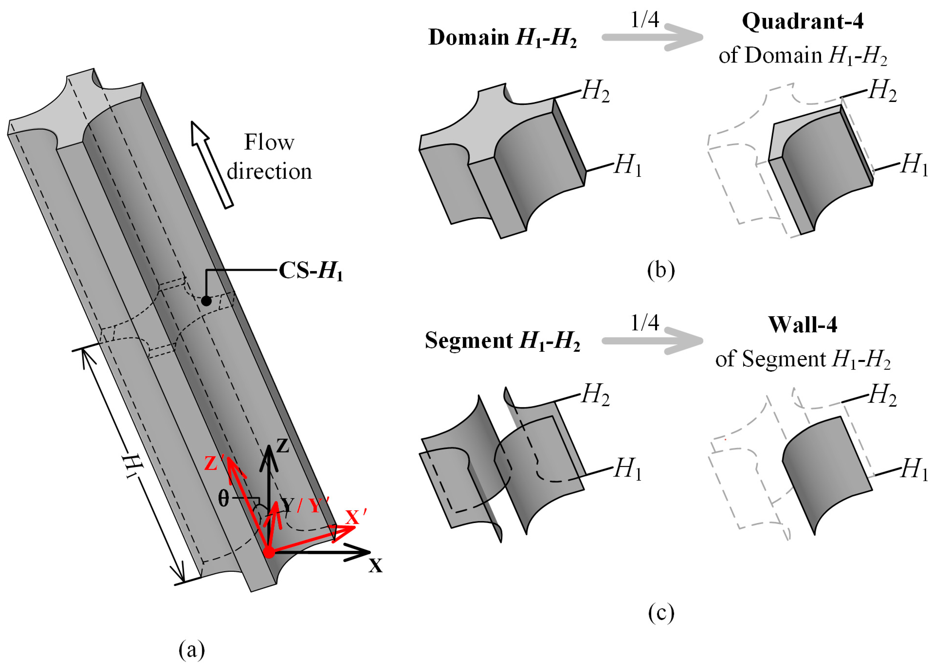
3.1.1. Transverse Flow

The secondary flow is classified into two kinds by the physical mechanism [33]. Secondary flows of the first kind, driven by pressure, occur in both laminar and turbulent flows. Secondary flows of the second kind due to the non-isotropic Reynolds stress distribution only occur in turbulent flow in straight pipes of a noncircular cross-section. In the present study, these two kinds of secondary flows both exist under the effect of cross-section, boiling, and rolling motion. This flow perpendicular to the main direction of fluid motion is referred to here as transverse flow. 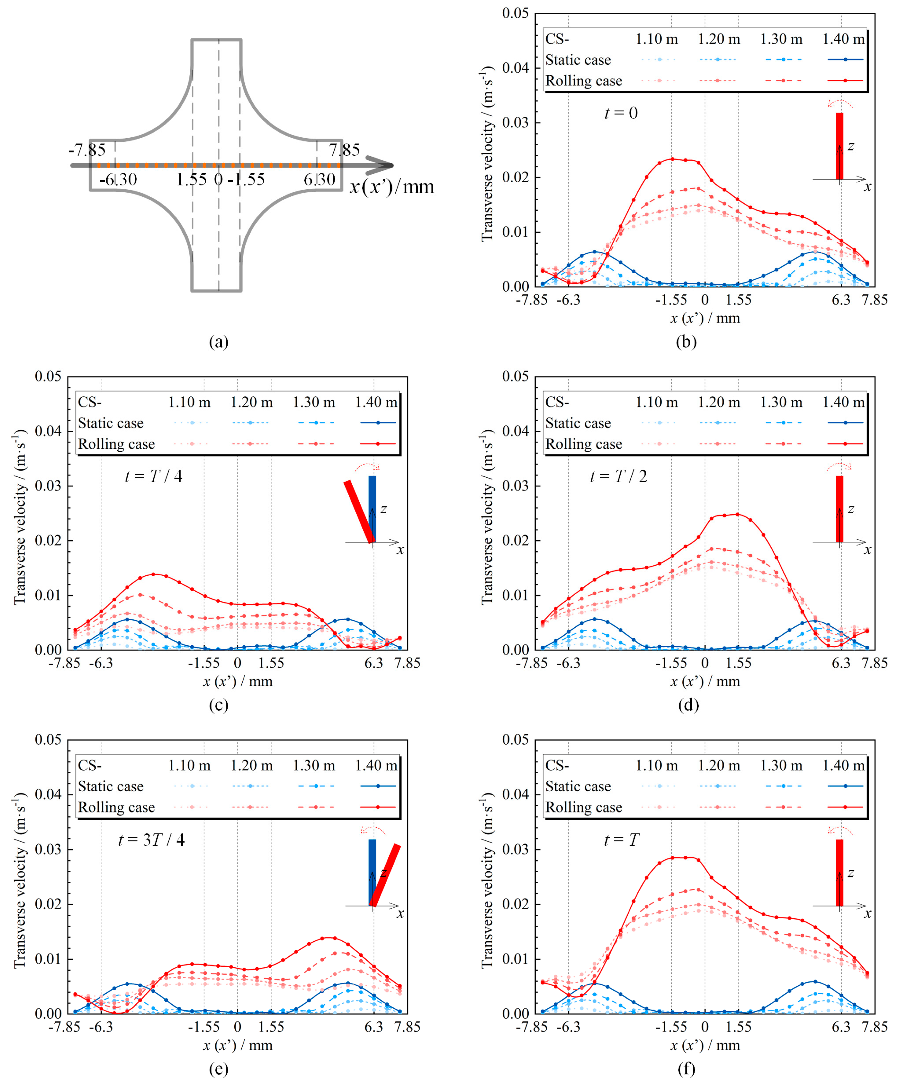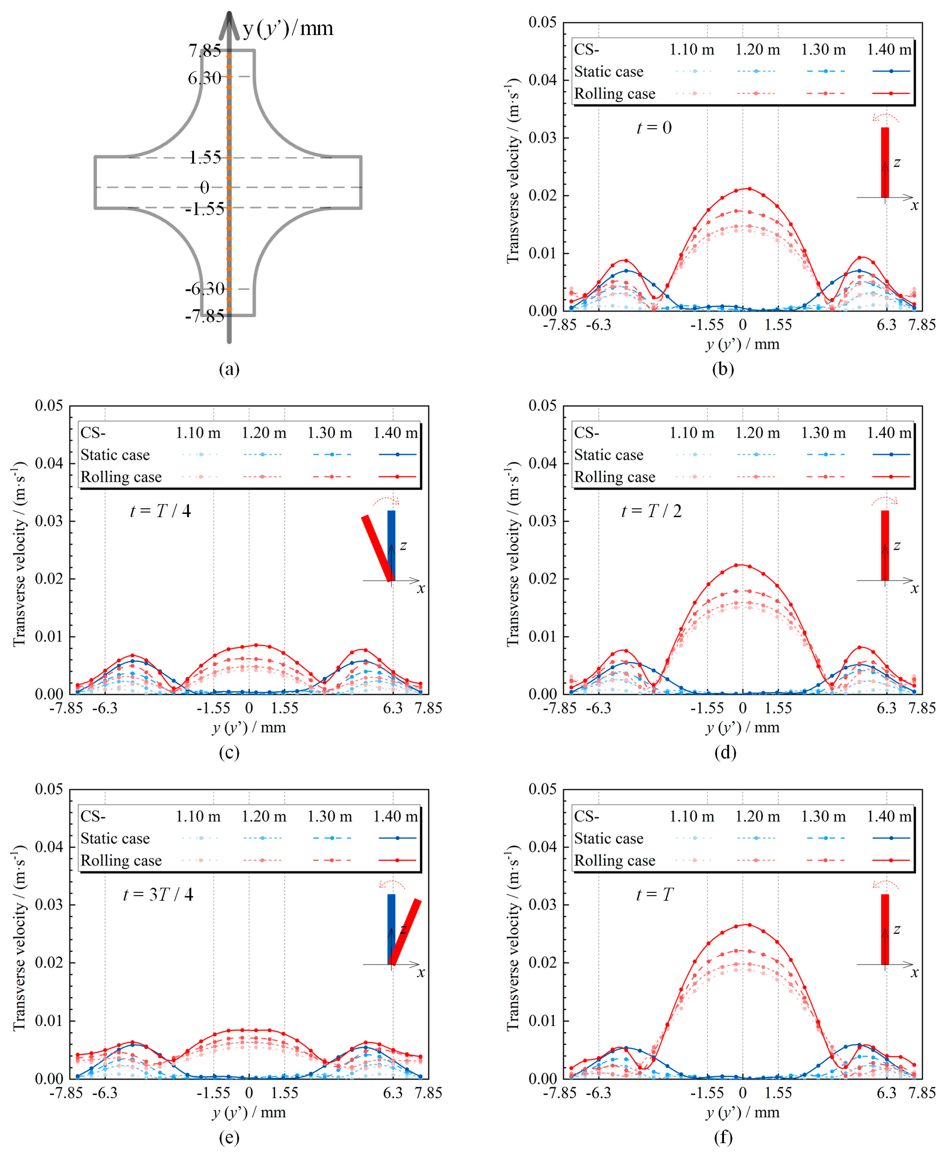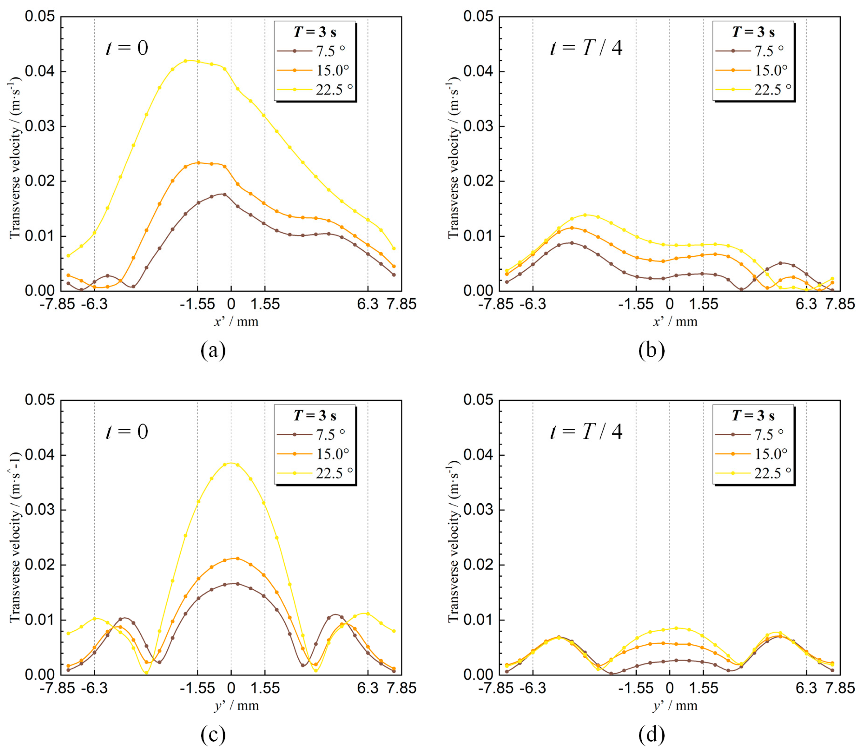Figure 3 depicts the transverse velocities on the $x$-axis ($x{}^{\prime }$-axis) of CS-1.10 m, CS-1.20 m, CS-1.30 m, and CS-1.40 m. The transverse velocities on the $y$-axis ($y{}^{\prime }$-axis) are shown in Figure 4.

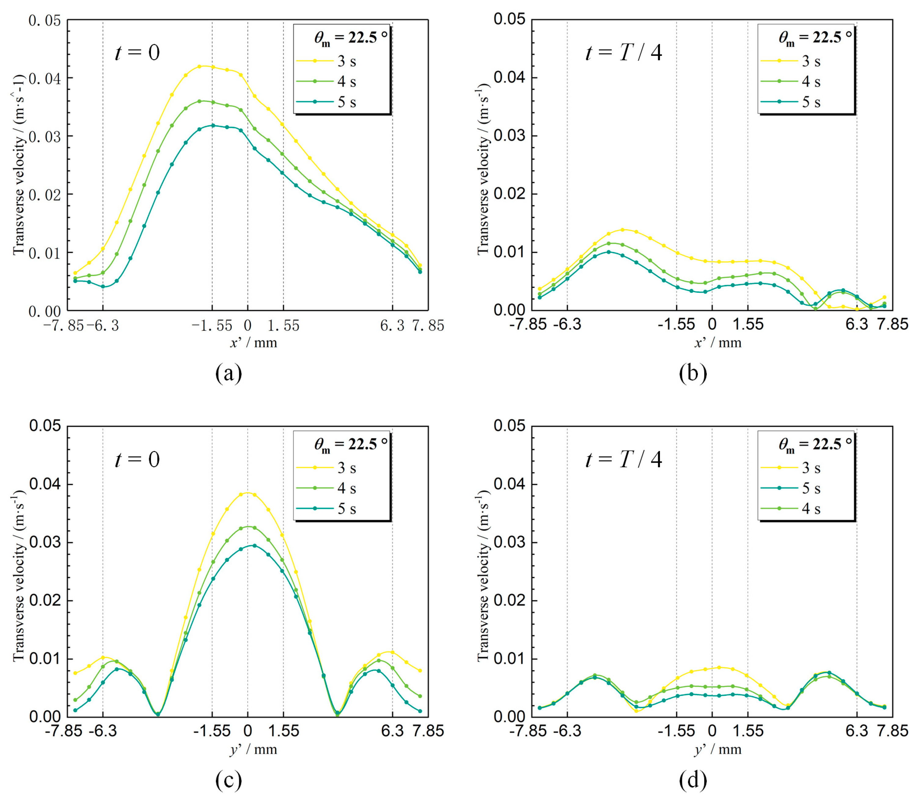
The transverse velocities in all the cross-sections are nearly constant with time under static state. The profiles of the transverse velocity on the $x$-axis and the $y$-axis are similar and feature two peaks. The transverse velocities are almost zero in the middle of the cross-section, whereas they reach the peaks in the rod gap. The transverse velocities in the rod gap increase with the height of the cross-section.

The transverse velocities under rolling motion differ significantly from those under static state. They change periodically. Firstly, transverse velocity profiles at the beginning of the period (Figure 3b and Figure 4b) are almost the same as those at the end (Figure 3f and Figure 4f). Secondly, the profiles of the transverse velocity on the $x{}^{\prime }$-axis at the moments $t$ and $t+T/2$ are symmetric with respect to the $y{}^{\prime }$-axis. Thirdly, when the subchannel is in the equilibrium position, which is the same as that under static state, the transverse velocity under rolling motion is far more than that under static state, especially in the middle of the cross-section (Figure 3b,d).

The above-mentioned transverse flow is induced mainly by boiling and rolling motion. The liquid subcooling is too high to permit bubble nucleation near the subchannel inlet. The heat transfer regime is forced convection. With increasing height, boiling initiates when the liquid in the vicinity of the heated surface reaches saturated. Mass transfer between the liquid phase and the vapor phase and the disturbance of bubbles lead to transverse flow inside the subchannel.

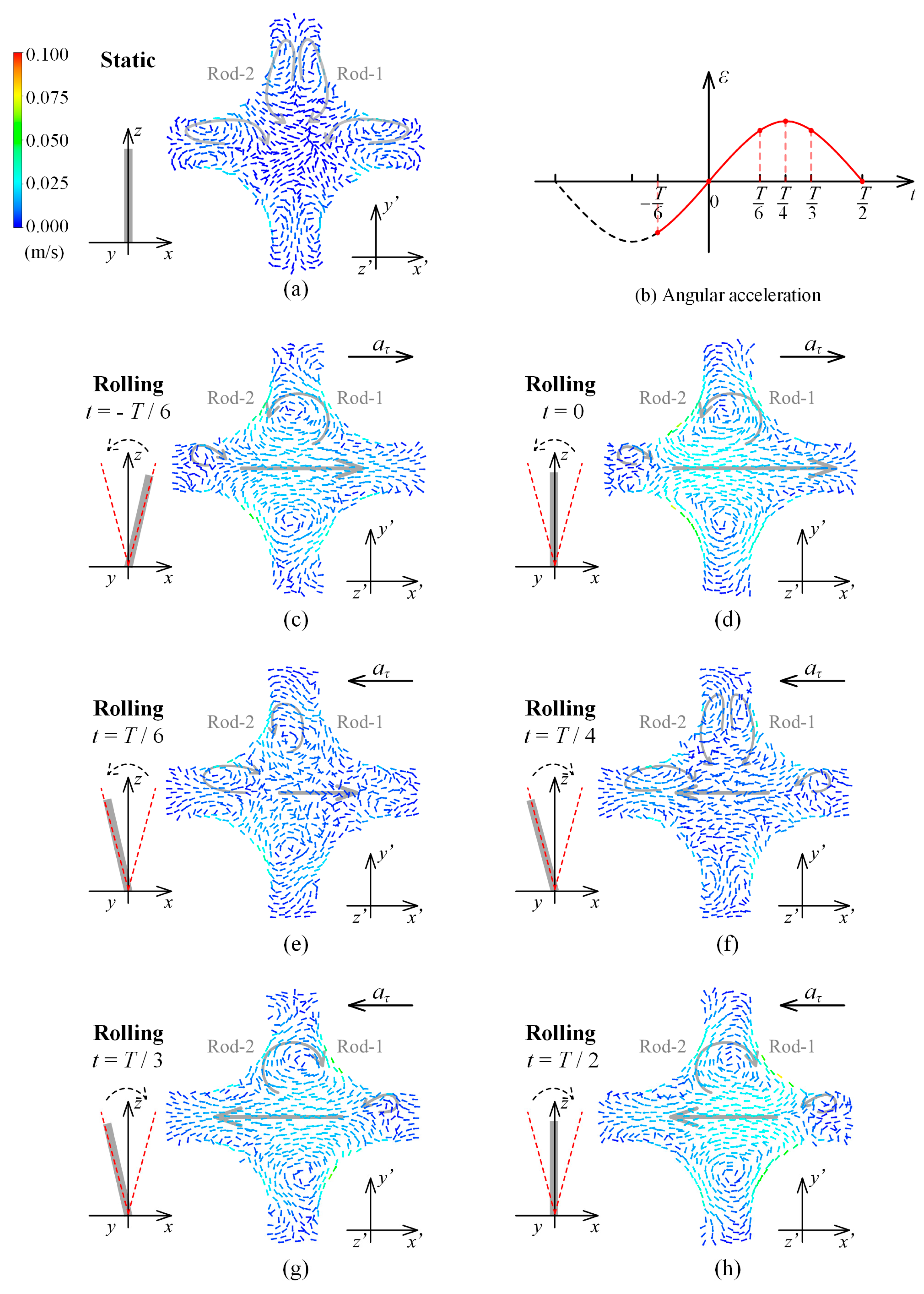
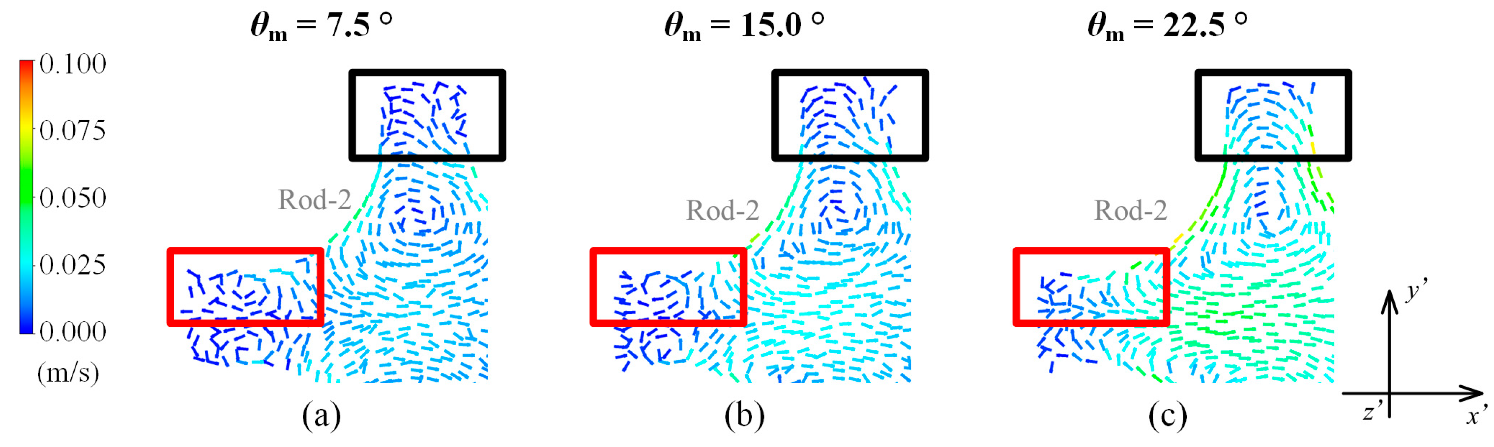
Under static state, due to the symmetrical geometry of the subchannel, the transverse velocity fields at the cross-sections are axially symmetrical with two vortices rotating reversely in the rod gaps (Figure 5a), with a sketch of the subchannel in the lower left corner). A similar transverse flow field is also obtained in Bieder et al.’s study [34]. Further downstream, the nucleate boiling intensifies, and the transverse velocity increases. The nucleate boiling occurs only in the vicinity of the heated surface while the bulk liquid is still subcooled. As a result, there is almost no transverse flow at the cross-section center under static state. Moreover, flow and heat transfer in the subchannel are stable, and the transverse flow is independent of time.

Boiling will promote the transverse flow of fluid, whereas rolling motion has a predominant role under rolling motion. The formation and evolution of the transverse flow under rolling motion are interpreted with the transverse flow fields.

When the subchannel rotates anticlockwise to the equilibrium position, the angular acceleration is negative (Figure 5b), and the Euler force on the fluid is positive along the $x{}^{\prime }$-axis (Equation (11)). Meanwhile, a region consisting of the middle of the cross-section and the two gaps around the $x{}^{\prime }$-axis is free of wall impediment. Fluid in this open region flows along the $x{}^{\prime }$-axis to the positive direction under the action of the Euler force, and two secondary vortices of the reverse direction emerge at the cross-section (Figure 5c). On the negative side of the $x{}^{\prime }$-axis, the transverse velocity induced by boiling and rolling motion is in the opposite direction. Therefore, the secondary vortex on the negative side of the $x{}^{\prime }$-axis is weakened by the rolling motion and smaller than that under static state. On the positive side of the $x{}^{\prime }$-axis, the secondary vortex induced by boiling merges into that induced by rolling motion because of the same direction.

When the subchannel reaches the equilibrium position ($t=0$), the Euler force decreases to zero. The transverse velocity in the middle of the cross-section reaches the maximum, far more than that under static state, whereas the secondary vortices in the middle still prevail at the cross-section (Figure 5d). The maximum transverse velocity on the $x{}^{\prime }$-axis occurs in the vicinity between Rod-2 and Rod-3 due to the promotion of boiling. Under the effect of boiling and rolling motion, transverse flow in the connected area comes up. However, the velocity profiles differ between the two sides of the $x{}^{\prime }$-axis due to the combined effect of boiling and rolling motion. On the two sides of the $y{}^{\prime }$-axis, the transverse velocity is slightly greater than that under static state, but rapidly decreases to zero near the middle of the secondary vortices.

Then, the subchannel rotates anticlockwise to the extreme position. The angular acceleration is positive during this process, and the Euler force on the fluid is negative along the $x{}^{\prime }$-axis. Transverse velocity around the $x{}^{\prime }$-axis decreases gradually and then increases reversely, and new secondary vortices emerge (Figure 5e). In the meantime, transverse velocity around the positive and negative sides of the $y{}^{\prime }$-axis also decreases gradually, and the effect of boiling on the transverse flow field comes into view gradually.

When the subchannel reaches the extreme position ($t=T/4$), the Euler force increases to its maximum. The transverse flow field is similar to that under static state (Figure 5f). However, the transverse velocity at this time is far less than that at the other moments in the rolling motion process. The transverse velocity around the negative side of the $x{}^{\prime }$-axis is strengthened due to the same direction of the transverse flow induced by boiling and rolling motion. In contrast, the transverse velocity around the positive side is weakened due to the opposite direction. Consequently, transverse velocity on the $x{}^{\prime }$-axis decreases along the positive direction. The rolling motion almost does not affect the transverse flow around the positive and negative sides of the $y{}^{\prime }$-axis. Two secondary vortices are formed in the rod gap, and the transverse velocity profile is the same as that under static state.

Next, the subchannel changes to rotate clockwise from the extreme position to the equilibrium position. During this process, the angular acceleration and the Euler force on the fluid still point to the $x{}^{\prime }$-axis in the positive and negative directions, respectively. The transverse velocity in the middle of the cross-section increases, and two secondary vortices of reverse direction emerge (Figure 5g). When the subchannel reaches the equilibrium position ($t=T/2$) again, the Euler force is zero, and the transverse velocity in the middle of the cross-section increases to its maximum. The two transverse velocity profiles on the $x{}^{\prime }$-axis are symmetrical around the axis of $x{}^{\prime }$ = 0 (Figure 5h).

The evolution of the transverse flow during the next half period is similar to those during the above-mentioned first half period.

3.1.2. Vapor Volume Fraction

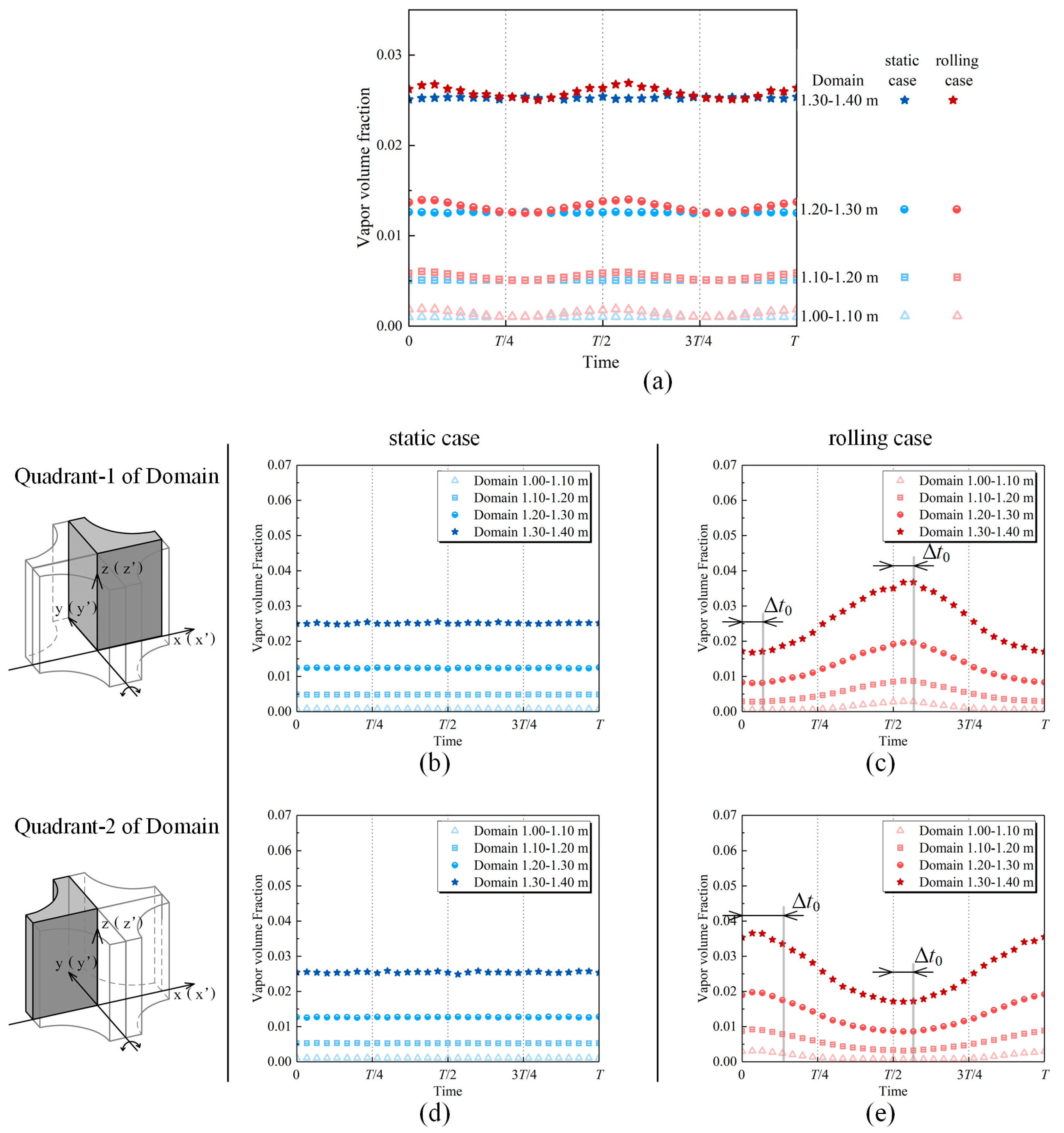
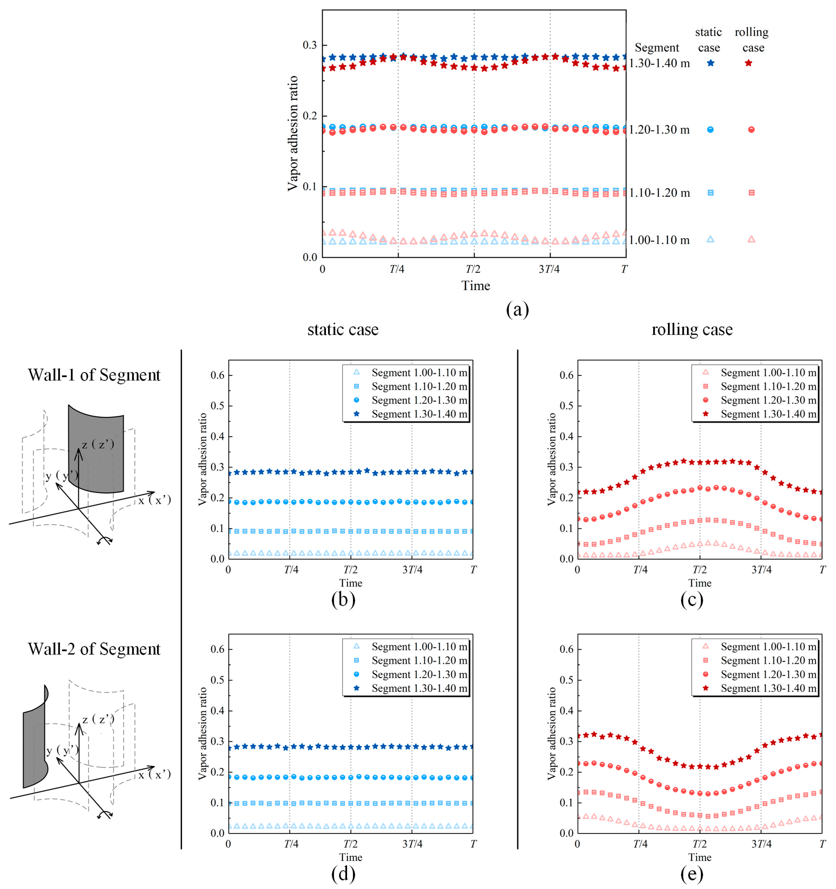
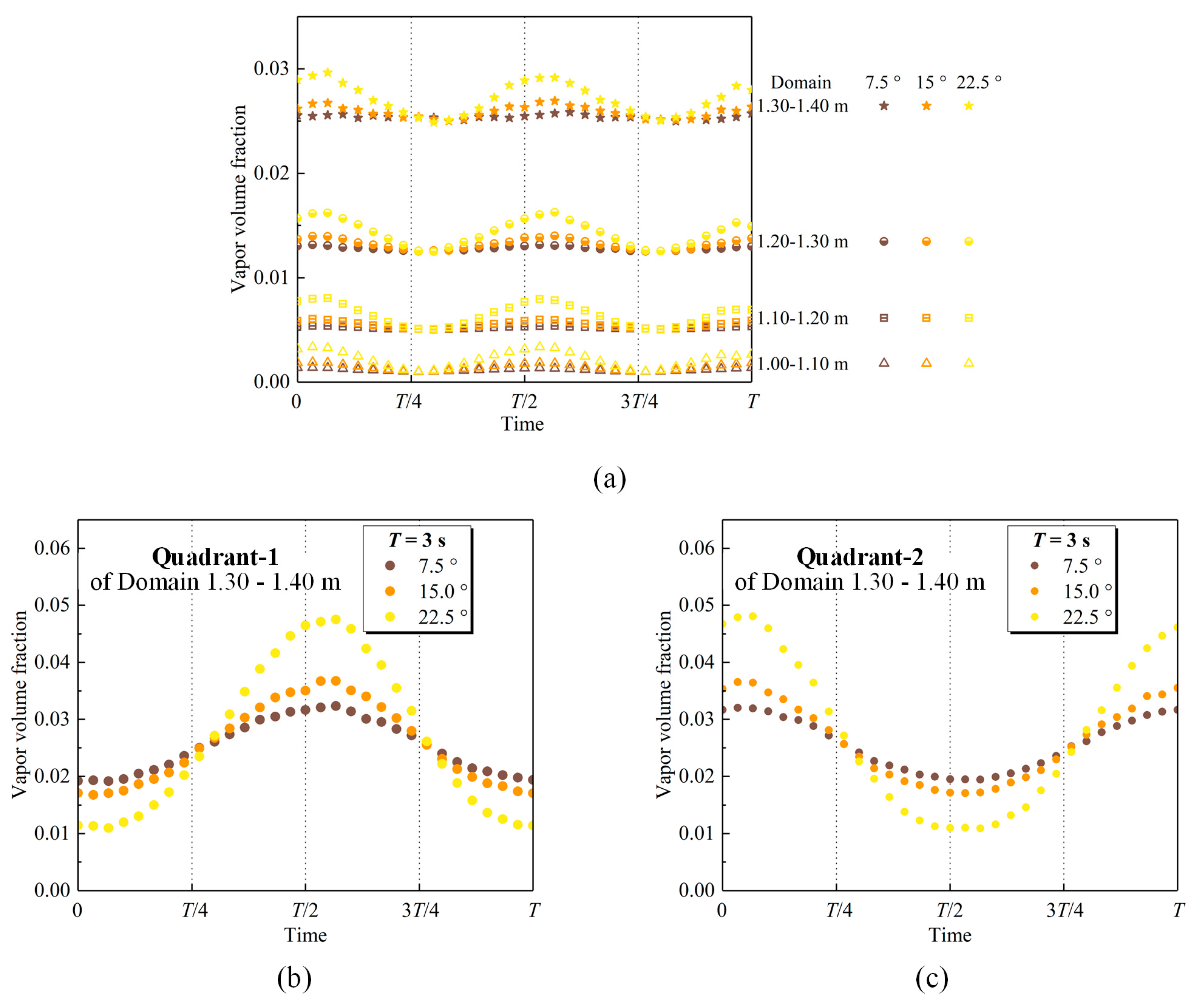
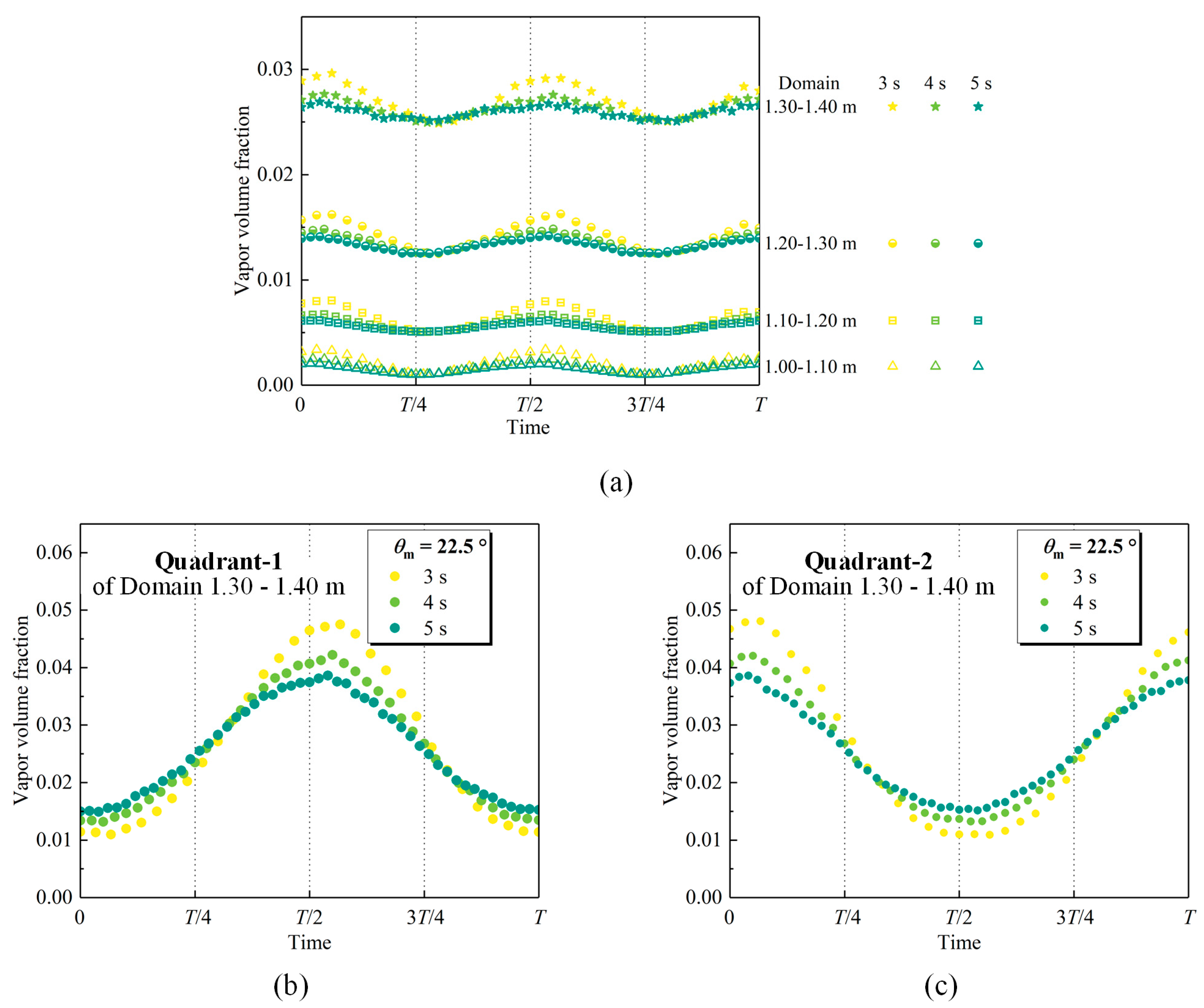
Transverse flow under static state is very different from that under rolling motion, as is vapor volume fraction in the two-phase domain. Tendencies of vapor volume fraction in the domain are shown in Figure 6a, in which the vapor volume fraction is the area-averaged value in each domain of 0.10 m height. The results in four domains from CS-1.00 m to CS-1.40 m are displayed. At any moment, the vapor volume fraction increases along the flow direction in the static and the rolling cases. However, the tendencies of the vapor volume fraction are different. The vapor volume fraction in each domain is constant under static state, whereas it oscillates under rolling motion. The period of vapor volume fraction under rolling motion is almost half that of the rolling motion. Moreover, vapor volume fraction under rolling motion is always greater than that under static state for each domain.

Under static state, the vapor volume fraction in Quadrant-1 and Quadrant-2 are constant and approximately equal to each other (Figure 6b,d). The tendency of vapor volume fraction in each quadrant features a similar pattern to that of the whole domain. The vapor volume fraction increases along the flow direction in both quadrants. Under rolling motion, the tendency of the vapor volume fraction in each quadrant differs from that in the whole domain (Figure 6c,e). In each domain, vapor volume fraction in both quadrants oscillates with the period equal to that of rolling motion but is in phase opposition.

The difference in vapor volume fraction between the static and rolling case is primarily attributed to the difference in transverse flow field. The transverse flow fields in both the quadrants are similar and constant with time under static state, whereas they differ significantly and oscillate periodically under rolling motion. The reason is explained below in chronological order.

The transverse flow pattern at the cross-section remains the same during the process when the subchannel rotates anticlockwise to the equilibrium position. Highly subcooled bulk fluid flows successively by Rod-1 and Rod-2, and the fluid temperature nearby Rod-1 is lower. As a result, the vapor volume fraction in Quadrant-1 is far less than that in Quadrant-2 when the subchannel is in the equilibrium position ($t=0$), when $t=\mathsf{\Delta }{t}_0$. The vapor volume fraction in Quadrant-1 and Quadrant-2 reaches the minimum and the maximum, respectively. After that, the subchannel continues to rotate anticlockwise, and the transverse flow field begins to reverse. A portion of the bulk fluid and fluid in the connected area flow to the vicinity of Rod-2. Bubbles in Quadrant-2 condense quickly, leading to vapor volume fraction decreases therein. A portion of the bulk fluid still flows to the vicinity of Rod-1. However, the flow rate decreases with time, and the vapor volume fraction increases therein. When the subchannel reaches the extreme position ($t=T/4$), the vapor volume fractions in Quadrant-1 and Quadrant-2 are approximately equal to their values under static state. After that, the subchannel rotates clockwise, and the transverse flow pattern at the cross-section does not change after $t=T/3$ (Figure 5g,h). Highly subcooled bulk fluid flows successively by Rod-2 and Rod-1, and the bulk fluid temperature nearby Rod-1 is higher. As a result, the vapor volume fraction continues to decrease in Quadrant-1 and increase in Quadrant-2.

The tendencies of vapor volume fraction in both quadrants in the next half period reversed those in the above-mentioned first half period.

Noteworthy, in the rolling case, the vapor volume fraction in Quadrant-1 and Quadrant-2 oscillates around that under static state and is in phase opposition. The summation of the vapor volume fraction in each quadrant, i.e., the vapor volume fraction in a domain, is equal to or greater than that in the static case. This is because the increment under rolling motion is larger than the decrement all the time. Especially in Domain 1.0–1.1 m, the vapor volume fraction in each quadrant is equal to or greater than that under static state due to the lower position where the boil begins.

3.1.3. Vapor Adhesion Ratio

For subcooled flow boiling in the subchannel, the vapor volume fraction remains small in the computation domain and typically no more than a few percent. However, the bubbles adjacent to the wall may crowd sufficiently, and a growing bubble layer may form eventually. The departure from nucleate boiling (DNB) occurs without a sustained macroscopic contact between the liquid and the surface, even though the bulk flow in the subchannel may still be highly subcooled. Predictions of the vapor volume fraction and vapor adhesion are essential. The vapor adhesion ratio at the wall can be defined as

$$R=\frac{{{\displaystyle \int }}_{\mathrm{vapor}}^{}dA}{{{\displaystyle \int }}_{\mathrm{wall}}^{}dA}$$

(20)

The denominator denotes the area of the wall, and the numerator denotes the area of the wall covered with vapor.

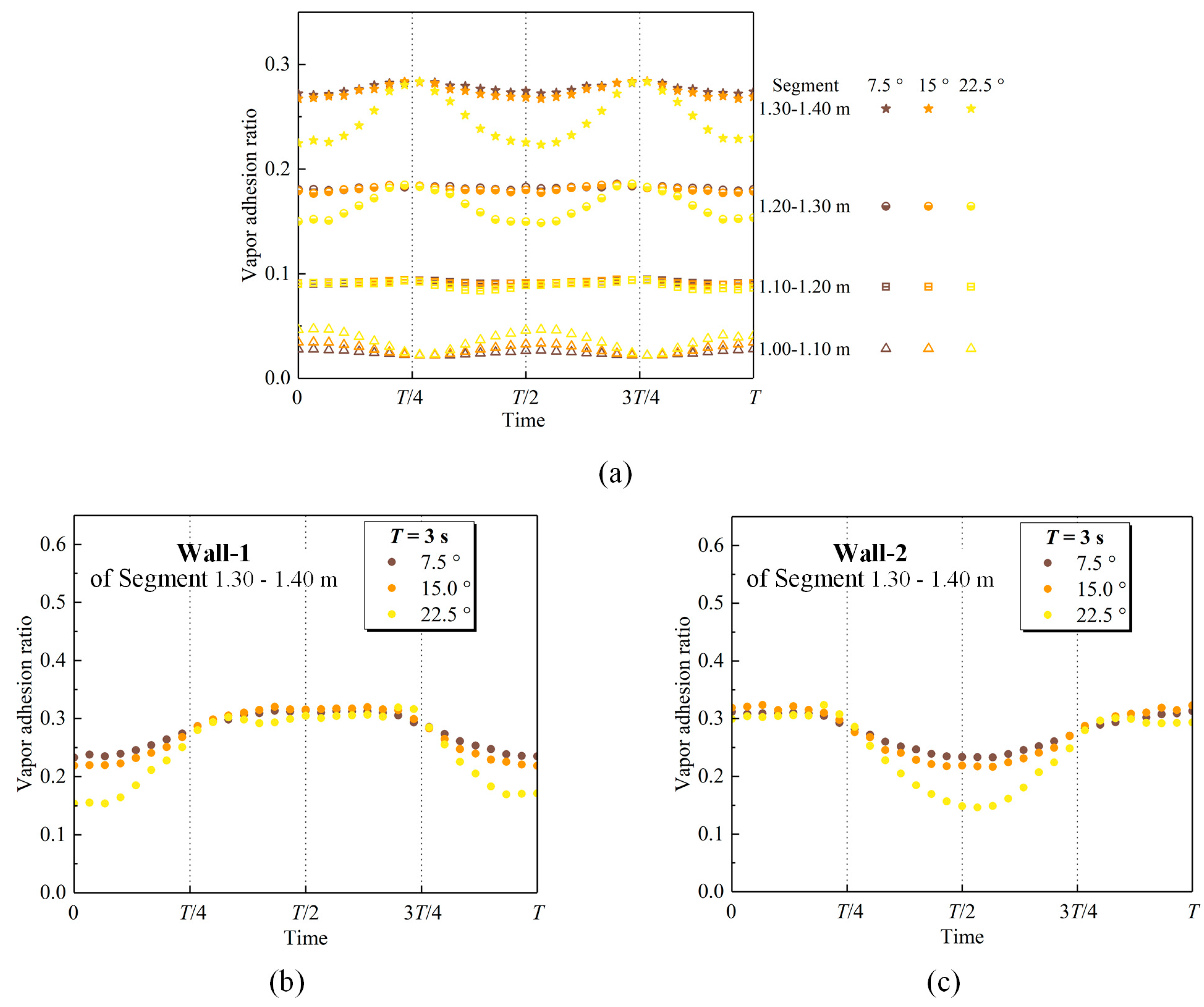
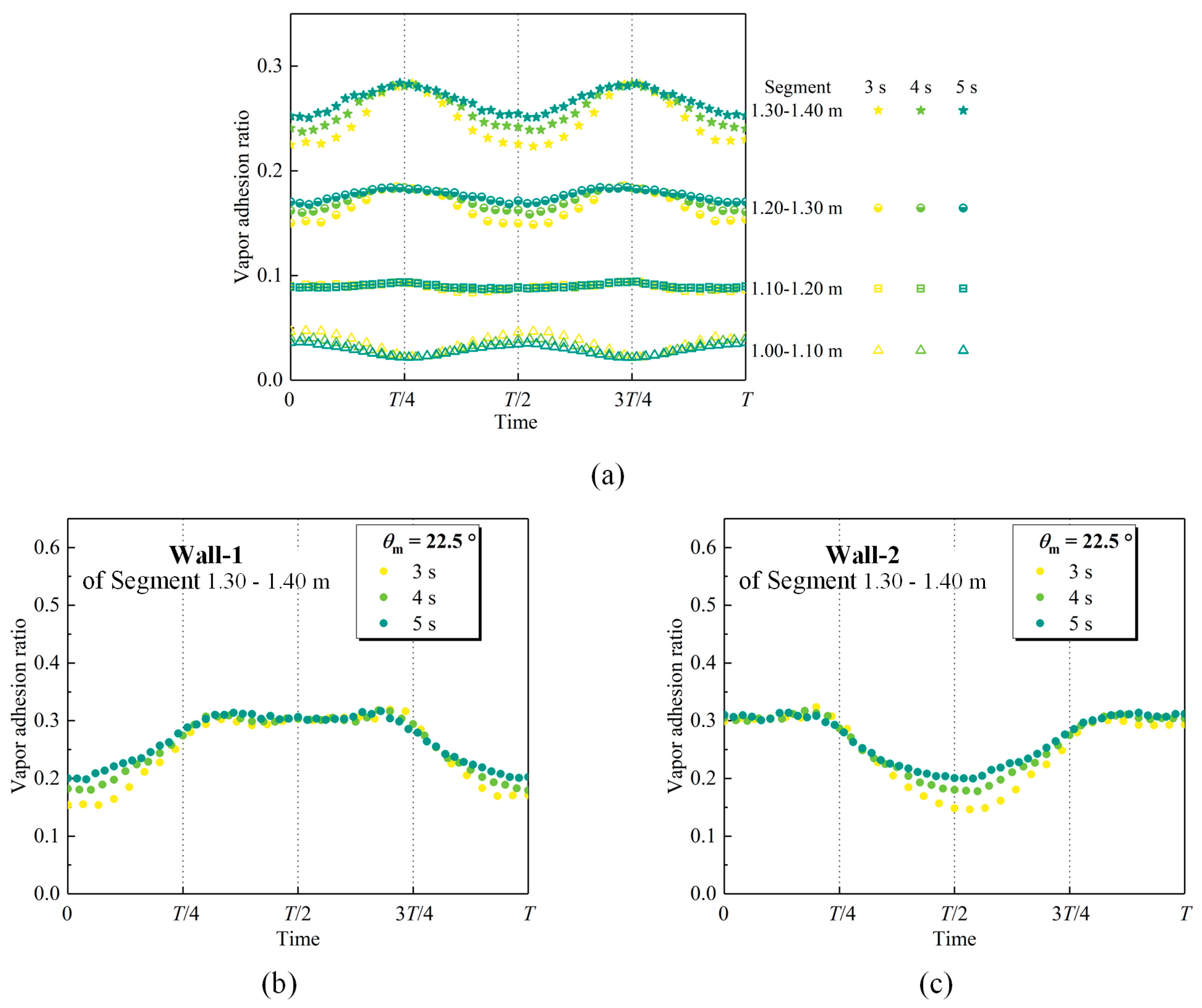
The tendencies of the vapor adhesion ratio at the wall are shown in Figure 7a. The vapor adhesion ratio is an area-averaged value at the wall, including both the heated and unheated surface in each domain 0.1 m high. It is defined in this way because the bubbles can not only be formed adjacent to the heated surface but also be pushed to the unheated surface. The vapor adhesion ratios increase along the flow direction under both static and rolling cases. The vapor adhesion ratio of Segment 1.00–1.10 m under rolling motion is greater than that under static state, whereas the vapor adhesion ratio of Segment 1.10–1.40 m is lower than that under static state.

For the static case, all the walls have axial symmetry, and the vapor adhesion ratio at them is identical and stable (Figure 7b,d). For the rolling case, the vapor adhesion ratios at both walls oscillate with a period equal to that of rolling motion (Figure 7c,e). Interestingly, the vapor adhesion ratio at Wall-2 is essentially constant when the vapor adhesion ratio at Wall-1 decreases or increases, and vice versa.

The vapor adhesion ratio at each wall increases along the flow direction. The effect of the transverse flow on the vapor adhesion ratio is slight at the lower position (Segment 1.00–1.20 m) under rolling motion. In Segment 1.00–1.10 m, the variation in the vapor adhesion ratio with time can be divided into three phases on both walls: increase, constant, and decrease. Furthermore, the vapor adhesion ratios under rolling motion are always greater than those under static state on both walls. They oscillate with the period half as much as that of rolling motion. In Segment 1.10–1.20 m, the vapor adhesion ratios under rolling motion on both walls oscillate around that under static state.

The tendencies of the vapor adhesion ratio are different at the upper position (Segment 1.20–1.40 m) due to the combined effects of the vapor volume fraction and the transverse flow. At the beginning of rolling motion ($t=0$), the vapor adhesion ratio at Wall-1 is less than that under static state due to transverse flow. Then, it gradually increases to approximately the value under static state when the subchannel reaches the extreme position ($t=T/4$). After that, the incoming fluid temperature in the vicinity of Rod-1 begins to increase, and more fluid reaches saturated to boil. In the meantime, the vapor volume fraction in Quadrant-1 and the vapor adhesion ratio at Wall-1 increase.

When the subchannel rotates anticlockwise from the extreme to the equilibrium position, the vapor volume fraction in Quadrant-1 increases continuously, and bubbles on the heated surface shift along the transverse flow. Finally, a great quantity of bubbles accumulate near the boundary between the heated surface and the unheated surface by the entrainment and flush of transverse flow. The vapor layer thickness increases as the vapor volume fraction increases, while the vapor adhesion ratio is constant (Figure 7d). The subcooled fluid in the middle of the cross-section and the gap between Rod-1 and Rod-2 flows to Rod-1 after the subchannel reaches the equilibrium position ($t=T/2$). The vapor volume fraction in Quadrant-1 decreases gradually. The bubbles, far from the heated surface in the boundary between the heated surface and the unheated surface, are apt to be affected by transverse flow and begin to condense. Therefore, the maximum vapor layer thickness at Wall-1 decreases while the vapor adhesion ratio is constant.

When the subchannel reaches the extreme position again ($t=3T/4$), the transverse velocity in the vicinity of Rod-1 begins to increase. After that, the vapor volume fraction in Quadrant-1 decreases gradually. The bubbles shift to the center of the heated surface slowly, which leads to the decrease in the vapor adhesion ratio at Wall-1.

The tendencies of the vapor adhesion ratio at other walls follow the same pattern as that at Wall-1. In conclusion, although the vapor volume fraction under rolling motion is always higher than that under static state at the upper position of the flow domain, the transverse flow tends to cause bubble accumulation, and the vapor adhesion ratio is less than that under static state all the time.

3.1.4. Phase Distribution

For PWRs at normal operation, local boiling occurs at a higher elevation of the reactor core. Vapor bubbles grow attached to the fuel rod while the bulk flow is still highly subcooled. As the height increases, multiple bubbles coalesce to form thin and discontinuous vapor layers. Therefore, the flow pattern in the present study is quite different from that in saturated boiling. In addition, the phase distribution in the subchannel is significantly different from that in the circular and rectangular tubes under the effect of the geometrical configuration.

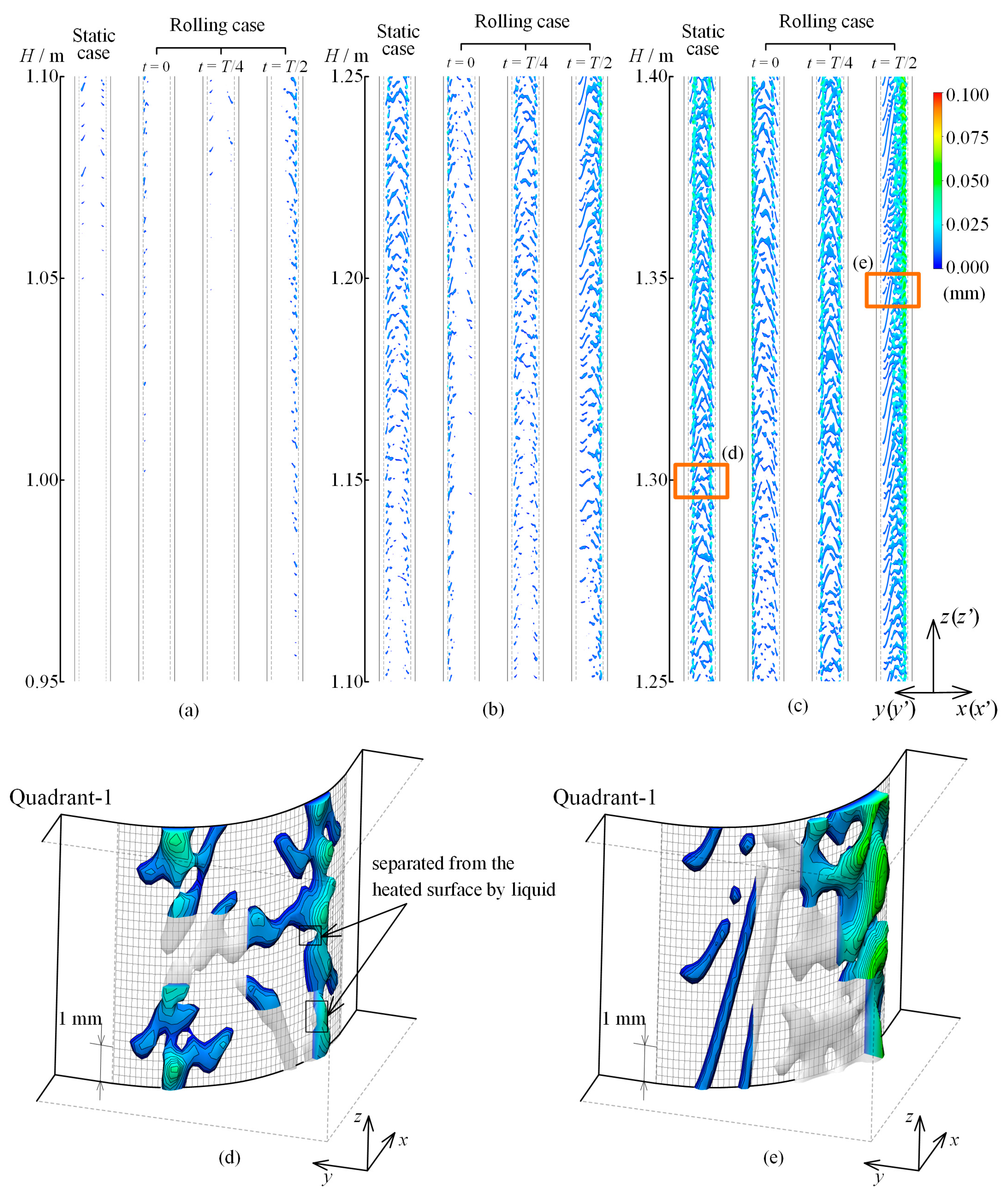
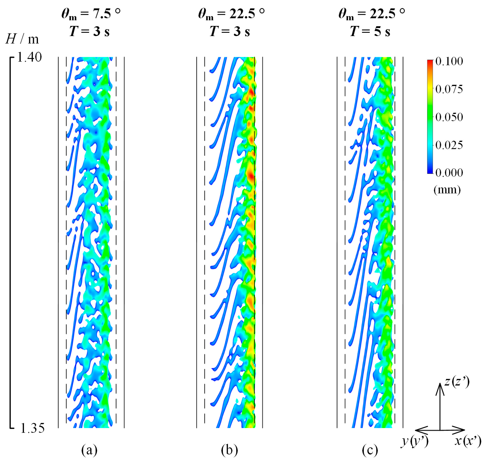
The vapor–liquid phase distribution in Quadrant-1 is shown in Figure 8. Only the vapor phase is shown in the figure, with color indicating the perpendicular distance between the interface and the heated surface. The region inside the black dashed line is the heated surface. The regions between the continuous and dashed lines are the rectangular unheated surfaces adjacent to the rod.

Flow and heat transfer in the subchannel are stable under static state. The OSV occurs around CS-1.05 m. Even though the heat flux of the fuel rod is uniform, fluid along both sides of the heated surface reaches saturated earlier under the effect of the channel sectional configuration (Figure 8a).

As the height increases, fluid along both sides and the center of the heated surface begins to boil (Figure 8b). The bubble is not the typical sphere but is long and narrow due to the transverse flow (Figure 5a). The fluid near the heated surface flows from both sides to the center, and the bubbles will be elongated to incline towards the center of the heated surface. Some bubbles will break into multiple small bubbles to merge with bubbles in the center of the heated surface. Bubbles in the center of the heated surface will grow continuously and bridge bubbles on both sides.

Further downstream, two vapor columns come into being due to more bubbles accumulating on both sides of the heated surface (Figure 8c). It should be emphasized that part of the vapor column herein is separated from the heated surface by liquid and does not cover the heated surface absolutely (Figure 8d). Vapor near the surface is submerged in the boundary layer with low velocity, and vapor far away from the surface flows downstream with high velocity. They detach from each other due to the velocity difference. Vapor far away from the surface interconnects together as a column, whereas the vapor phase and the liquid phase are separated near the surface.

Under rolling motion, the vapor–liquid phase distribution in the subchannel varies with time due to transverse flow, which features the following characteristics. When the subchannel reaches the equilibrium position ($t=0$ or $t=T/2$), which is the same as that under static state, the phase distribution is significantly different from that under static state. The OSV point under rolling motion is much lower than that under static state (Figure 8a). Further downstream, vapor bubbles are swept by the transverse flow and the amount of the vapor increases along the direction of the transverse flow. Although the transverse flow fields are similar when $t=0$ and $t=T/2$, the phase distributions are slightly different. Different directions of the transverse flow not only result in different positions where bubbles accumulate but also affect the vapor volume fraction. When $t=T/2$, transverse flow heated by Rod-2 then flows to Rod-1, causing more liquid to boil (Figure 8e). Bubbles on the left side of the heated surface grow in length and eventually break into discrete bubbles. Multiple bubbles on the right side coalesce and collect at the boundary of the heated and unheated surface. When the subchannel reaches the extreme position ($t=T/4$ or $t=3T/4$), the vapor–liquid phase distribution is similar to that under static state due to a similar transverse flow field.

3.2. Sensitivity Analysis

3.2.1. Transverse Flow

The effects of the amplitude on the transverse flow are shown in Figure 9, taking the transverse velocity in CS-1.40 m as an example. The transverse flow velocity distributions are similar for different amplitudes. The rolling motion dominates the transverse flow in the middle of the cross-section at any time. Therefore, the Euler force increases as the amplitude increases. So, the transverse velocity in the middle of the cross-section increases. The transverse flow in other locations is dominated by both boiling and rolling motion.

The transverse velocity in the middle of the cross-section is in the positive direction of the $x{}^{\prime }$-axis when the subchannel is in the equilibrium position ($t=0$). On the negative side of the $x{}^{\prime }$-axis, the transverse flow is in the negative $x{}^{\prime }$-axis direction. For the small amplitude (7.5°), the transverse velocity induced by rolling motion is small, and the effect of boiling on the transverse flow is prominent. At this time, the transverse velocity profile is similar to that under static state. For the large amplitude (22.5°), the transverse velocity induced by rolling motion is large, and the effect of the rolling motion is dominant. The closer to the middle of the cross-section, the greater the transverse velocity. Figure 10 compares the transverse flow with different amplitudes of rolling motion. The secondary vortices induced by boiling still exist around the negative $x{}^{\prime }$-axis when the amplitudes are 7.5° and 15.0° but vanish thoroughly at 22.5° (the red box in Figure 10).

On the positive $x{}^{\prime }$-axis, the transverse flow induced by boiling is superimposed on that induced by rolling motion due to identical direction. The transverse velocity here increases as the amplitude increases.

On the $y{}^{\prime }$-axis, the transverse flow on the positive side is identical to that on the negative side. If the amplitude of rolling motion is small (7.5°), the transverse velocity induced by rolling motion is small, and the transverse flow on the $y{}^{\prime }$-axis is dominated by both boiling and rolling motion. The velocity profiles are approximately the same, but the magnitude is higher than that under static state. If the amplitude of rolling motion is large (22.5°), the effect of rolling motion on the transverse flow is prominent. The transverse flow induced by rolling is higher, especially on both ends of the $y{}^{\prime }$-axis. As can be seen from the black box in Figure 10, the secondary vortex is intensified gradually, and the center approaches the $y{}^{\prime }$-axis as the amplitude increases. When the amplitude is 22.5°, the location where the transverse velocity on y’-axial equals zero is the center of the secondary vortex.

The transverse velocity in the middle of the cross-section is in the negative direction of the $x{}^{\prime }$-axis when the subchannel is in the extreme position ($t=T/4$). On the $x{}^{\prime }$-axis, the transverse flow is dominated by both boiling and rolling motion. The transverse flow induced by boiling remains the same throughout. Hence, the rolling motion enhances the transverse flow on the negative $x{}^{\prime }$-axis and mitigates it on the positive side. As the amplitude increases, the transverse velocities on the negative and positive sides of the $x{}^{\prime }$-axis are in reverse. On the $y{}^{\prime }$-axis, the transverse flow is only dominated by boiling and independent of the amplitude of rolling motion.

The effects of the period on the transverse flow are depicted in Figure 11. The transverse velocity profiles are the same for different periods. The transverse flow in the middle of the cross-section is dominated by rolling motion all the time. Therefore, as the period decreases, the Euler force increases, as does the transverse velocity in the middle of the cross-section. In the other location of the cross-section, the transverse flow is dominated by both the boiling and rolling motion.

When the subchannel is in the equilibrium position ($t=0$), the transverse flows on both the $x{}^{\prime }$-axis and $y{}^{\prime }$-axis are dominated by the rolling motion. Therefore, the transverse flow velocity in the whole cross-section decreases as the period decreases, except that in the center of the secondary vortex is zero.

When the subchannel is in the extreme position ($t=T/4$), the effect of boiling on the transverse flow comes into view. On the $x{}^{\prime }$-axis, the transverse velocity on the negative side increases while that on the positive side decreases as the period decreases. The transverse flow on the $y{}^{\prime }$-axis is only dominated by boiling and independent of the period.

In summary, the Euler force is the fundamental reason for the variation in the transverse flow under rolling motion. It depends on the amplitude and period of rolling motion. The Euler force increases with the amplitude, decreases with the period, and vice versa. Consequently, the tendency of the transverse flow is the same when the amplitude increases or the period decreases.

3.2.2. Vapor Volume Fraction

The tendencies of vapor volume fraction are similar for different amplitudes of rolling motion in each domain (Figure 12a). The vapor volume fraction in each domain approaches the maximum when the subchannel deviates from the equilibrium position (about $t=0$ or $t=T/2$), and the minimum when it deviates from the extreme position (about $t=T/4$ or $t=3T/4$). The period of the vapor volume fraction is half that of rolling motion. As the amplitude of rolling motion increases, the maximum of the vapor volume fraction in each domain increases. For Domain 1.30–1.40 m, the maximum of the vapor volume fraction under rolling motion is 2.5%, 7.3%, and 17.5% larger than the time-averaged vapor volume fraction under static state when the amplitude is 7.5°, 15.0°, and 22.5°, respectively. However, the minimum is constantly equivalent to that in the same domain under static state.

The vapor volume fraction in different quadrants is analyzed, taking the vapor volume fraction in Domain 1.30–1.40 m as an example (Figure 12b,c). The tendencies of the vapor volume fraction in Quadrant-1 are similar for different amplitudes of rolling motion. The tendencies of the vapor volume fraction in Quadrant-2 are the same as those in Quadrant-1 but different in phase by 180°. When the subchannel deviates from the equilibrium position (about $t=0$ or $t=T/2$), the difference between the vapor volume fraction in Quadrant-1 and Quadrant-2 increases as the amplitude of rolling motion increases. When the subchannel deviates from the extreme position (about $t=T/4$ or $t=3T/4$), the vapor volume fraction in Quadrant-1 or Quadrant-2 is independent of the amplitude of the rolling motion. Therefore, the maximum of the vapor volume fraction in each domain increases while the minimum is unchanged as the amplitude of rolling motion increases.

Figure 13 depicts the vapor volume fraction variation with the rolling motion period. As discussed previously, the variation in the vapor volume fraction fundamentally results from the variation in the transverse flow induced by the Euler force. When the amplitude of rolling motion increases or the period decreases, the variation in the transverse flow is identical, and so is the vapor volume fraction.

3.2.3. Vapor Adhesion Ratio

The tendencies of the vapor adhesion ratio are similar for different amplitudes of rolling motion at each segment (Figure 14a). The vapor adhesion ratio at each segment approaches the minimum when the subchannel deviates from the equilibrium position (about $t=0$ or $t=T/2$), and the maximum when it deviates from the extreme position (about $t=T/4$ or $t=3T/4$). The period of the vapor adhesion ratio is half that of rolling motion. As the amplitude of rolling motion increases, the minimum of the vapor adhesion ratio at each segment decreases. For Segment 1.30–1.40 m, the minimum of the vapor adhesion ratio under rolling motion is 18.0%, 23.0%, and 45.9% smaller than the time-averaged vapor adhesion ratio under static state when the amplitude is 7.5°, 15.0°, and 22.5°, respectively. Nevertheless, the maximum is equivalent to that in the same segment under static state.

The vapor adhesion ratio at different walls is analyzed, taking the vapor adhesion ratio at Segment 1.30–1.40 m as an example (Figure 14b,c). The tendencies of the vapor adhesion ratio at Wall-1 are similar for different amplitudes of rolling motion. The minimum of the vapor adhesion ratio decreases, and the maximum is constant as the amplitude of rolling motion increases. The tendencies of the vapor adhesion ratio at Wall-2 and Wall-1 are the same but different by a relative 180° phase shift. When the subchannel deviates from the equilibrium position (about $t=0$ or $t=T/2$), the difference between the vapor adhesion ratio at Wall-1 and Wall-2 increases as the amplitude of rolling motion increases. When the subchannel deviates from the extreme position (about $t=T/4$ or $t=3T/4$), the vapor adhesion ratio at Wall-1 or Wall-2 is independent of the amplitude of the rolling motion. Therefore, the minimum of the vapor adhesion ratio in each segment decreases while the maximum is unchanged as the amplitude of rolling motion increases.

Figure 15 depicts the vapor adhesion ratio variation with the rolling motion period. In addition to the vapor volume fraction, the variation in the transverse flow induced by the Euler force fundamentally results in the variation in the vapor adhesion ratio. Therefore, when the amplitude of rolling motion increases or the period decreases, the variation in the transverse flow is identical, as is the vapor adhesion ratio. Figure 16 shows the effect of the amplitude and the period on the vapor–liquid phase distribution in Quadrant-1 ($t=T/2$). The bubbles accumulate on the boundary of the heated and unheated surface when the subchannel is in the equilibrium position. When the amplitude increases or the period decreases, the bubble thickness increases, but the vapor adhesion ratio is basically constant.

4. Discussion

In the present study, we investigated the subcooled flow boiling in the subchannel under rolling motion following the trigonometric function. The tendency of physical parameters, including the transverse flow, volume fraction, and vapor adhesion ratio, was explored along the flow direction. The phase distribution in the two-phase flow domain is presented in this paper. The effects and mechanisms of the rolling motion parameters on the two-phase flow in the subchannel are analyzed. The main conclusions are as follows.

(1) The transverse flow under rolling motion is a composition of the boiling-induced and motion-induced transverse flow. The transverse flow induced by rolling motion fundamentally results from the Euler force in the non-inertial reference frame. The transverse flow in the center of the cross-section increases with the amplitude of the rolling motion and decreases with the period. The transverse flow in the other position of the cross-section depends on the rolling motion parameters and the position of the subchannel.

(2) The location of the OSV point and the vapor volume fraction in the two-phase flow domain varies with time because of the variation in the transverse flow. When the subchannel is around the equilibrium position, the volume fraction reaches the maximum, which increases with the amplitude of the rolling motion and decreases with the period. When the subchannel is about the extreme position, the volume fraction reaches the minimum, which is insensitive to the rolling motion parameters.

(3) In the present study, the vapor adhesion ratio upstream of CS-1.20 m is only related to the volume fraction, while the downstream is affected by both the volume fraction and the transverse flow. For the flow domain downstream of CS-1.20 m, the vapor adhesion ratio in the downstream reaches the minimum when the subchannel is around the equilibrium position. This minimum decreases with the amplitude of the rolling motion and increases with the period. The vapor adhesion ratio in the downstream reaches the maximum when the subchannel is about the extreme position. The maximum is insensitive to the rolling motion parameters.

(4) When the rolling motion parameters change, the phase distribution is similar at the same time under rolling motion. In the present study, bubbles slide to the boundary of the heated and unheated surface. The bubble thickness at this boundary increases with the amplitude of the rolling motion and decreases with the period.

References

1. Yan, C.; Yan, C.; Sun, L.; Xing, D.; Wang, Y. Investigation of the interfacial parameter distribution in a bubbly flow in a narrow rectangular channel under inclined and rolling conditions. Prog. Nucl. Energy 2014, 73, 64–74. [Google Scholar] [CrossRef]
2. Tanjung, E.F.; Kim, B.J.; Jo, D. Effects on pool boiling critical heat flux (CHF) with different direction and magnitude of additional accelerations due to rolling. Ann. Nucl. Energy 2021, 154, 108095. [Google Scholar] [CrossRef]
3. Hwang, J.-S.; Lee, Y.-G.; Park, G.-C. Characteristics of critical heat flux under rolling condition for flow boiling in vertical tube. Nucl. Eng. Des. 2012, 252, 153–162. [Google Scholar] [CrossRef]
4. Li, S.; Tan, S.; Gao, P.; Xu, C. Experimental research of bubble number density and bubble size in narrow rectangular channel under rolling motion. Nucl. Eng. Des. 2014, 268, 41–50. [Google Scholar] [CrossRef]
5. Li, S.; Tan, S.; Xu, C.; Gao, P. Visualization study of bubble behavior in a subcooled flow boiling channel under rolling motion. Ann. Nucl. Energy 2015, 76, 390–400. [Google Scholar] [CrossRef]
6. Kharangate, C.R.; Mudawar, I. Review of computational studies on boiling and condensation. Int. J. Heat Mass Transf. 2017, 108, 1164–1196. [Google Scholar] [CrossRef]
7. Choudhury, R.; Das, U.J.; Ceruti, A.; Piancastelli, L.; Frizziero, L.; Zanuccoli, G.; Daidzic, N.; Rocchi, I.; Casano, G.; Piva, S. Visco-elastic effects on the three dimensional hydrodynamic flow past a vertical porous plate. Int. Inf. Eng. Technol. Assoc. 2013, 31, 1–8. [Google Scholar] [CrossRef]
8. Valizadeh Yaghmourali, Y.; Ahmadi, N.; Abbaspour-sani, E. A thermal-calorimetric gas flow meter with improved isolating feature. Microsyst. Technol. 2016, 23, 1927–1936. [Google Scholar] [CrossRef]
9. Thome, J.R. (Ed.) Encyclopedia of Two-Phase Heat Transfer and Flow I Fundamentals and Methods Volume 4: Special Topics in Pool and Flow Boiling; World Scientific Publishing: Singapore, 2015; p. 176. [Google Scholar]
10. Jia, H.W.; Zhang, P.; Fu, X.; Jiang, S.C. A numerical investigation of nucleate boiling at a constant surface temperature. Appl. Therm. Eng. 2015, 88, 248–257. [Google Scholar] [CrossRef]
11. Cheng, N.; Guo, Y.; Peng, C. A numerical simulation of single bubble growth in subcooled boiling water. Ann. Nucl. Energy 2019, 124, 179–186. [Google Scholar] [CrossRef]
12. Bahreini, M.; Ramiar, A.; Ranjbar, A.A. Numerical simulation of bubble behavior in subcooled flow boiling under velocity and temperature gradient. Nucl. Eng. Des. 2015, 293, 238–248. [Google Scholar] [CrossRef]
13. Jeon, S.-S.; Kim, S.-J.; Park, G.-C. Numerical study of condensing bubble in subcooled boiling flow using volume of fluid model. Chem. Eng. Sci. 2011, 66, 5899–5909. [Google Scholar] [CrossRef]
14. Guo, L.; Zhang, S.; Hu, J. Flow boiling heat transfer characteristics of two-phase flow in microchannels. AIP Adv. 2022, 12, 055219. [Google Scholar] [CrossRef]
15. Cheng, N.; Yu, S.; Xiao, J.; Peng, C. Numerical simulation of single bubble growth in vertical rectangular narrow flow channels. Nucl. Eng. Des. 2022, 391, 111749. [Google Scholar] [CrossRef]
16. Pattamatta, A.; Freystein, M.; Stephan, P. A parametric study on phase change heat transfer due to Taylor-Bubble coalescence in a square minichannel. Int. J. Heat Mass Transf. 2014, 76, 16–32. [Google Scholar] [CrossRef]
17. Liu, Z.; Sunden, B.; Wu, H. Numerical Modeling of Multiple Bubbles Condensation in Subcooled Flow Boiling. J. Therm. Sci. Eng. Appl. 2015, 7, 031003. [Google Scholar] [CrossRef]
18. Lee, J.; O’Neill, L.E.; Mudawar, I. 3-D computational investigation and experimental validation of effect of shear-lift on two-phase flow and heat transfer characteristics of highly subcooled flow boiling in vertical upflow. Int. J. Heat Mass Transf. 2020, 150, 119291. [Google Scholar] [CrossRef]
19. Kuang, Y.W.; Wang, W.; Zhuan, R.; Yi, C.C. Simulation of boiling flow in evaporator of separate type heat pipe with low heat flux. Ann. Nucl. Energy 2015, 75, 158–167. [Google Scholar] [CrossRef]
20. Yin, X.; Tian, Y.; Zhou, D.; Wang, N. Numerical study of flow boiling in an intermediate-scale vertical tube under low heat flux. Appl. Therm. Eng. 2019, 153, 739–747. [Google Scholar] [CrossRef]
21. Devahdhanush, V.S.; Lei, Y.; Chen, Z.; Mudawar, I. Assessing advantages and disadvantages of macro- and micro-channel flow boiling for high-heat-flux thermal management using computational and theoretical/empirical methods. Int. J. Heat Mass Transf. 2021, 169, 120787. [Google Scholar] [CrossRef]
22. Darshan, M.B.; Kumar, R.; Das, A.K. Numerical study of interfacial dynamics in flow boiling of R134a inside smooth and structured tubes. Int. J. Heat Mass Transf. 2022, 188, 122592. [Google Scholar] [CrossRef]
23. Zhuan, R.; Wang, W. Flow pattern of boiling in micro-channel by numerical simulation. Int. J. Heat Mass Transf. 2012, 55, 1741–1753. [Google Scholar] [CrossRef]
24. Yang, Z.; Peng, X.F.; Ye, P. Numerical and experimental investigation of two phase flow during boiling in a coiled tube. Int. J. Heat Mass Transf. 2008, 51, 1003–1016. [Google Scholar] [CrossRef]
25. Amidu, M.A.; Addad, Y.; Riahi, M.K. A hybrid multiphase flow model for the prediction of both low and high void fraction nucleate boiling regimes. Appl. Therm. Eng. 2020, 178, 115625. [Google Scholar] [CrossRef]
26. Bahreini, M.; Ramiar, A.; Ranjbar, A.A. Numerical simulation of subcooled flow boiling under conjugate heat transfer and microgravity condition in a vertical mini channel. Appl. Therm. Eng. 2017, 113, 170–185. [Google Scholar] [CrossRef]
27. Lee, J.; Mudawar, I.; Hasan, M.M.; Nahra, H.K.; Mackey, J.R. Experimental and computational investigation of flow boiling in microgravity. Int. J. Heat Mass Transf. 2022, 183, 122237. [Google Scholar] [CrossRef]
28. Wang, L.; Wang, J.; Li, Y. CFD study on film boiling features of cryogenic fluid influenced by heat structures and gravity levels. Cryogenics 2022, 124, 103455. [Google Scholar] [CrossRef]
29. Wei, J.-H.; Pan, L.-M.; Chen, D.-Q.; Zhang, H.; Xu, J.-J.; Huang, Y.-P. Numerical simulation of bubble behaviors in subcooled flow boiling under swing motion. Nucl. Eng. Des. 2011, 241, 2898–2908. [Google Scholar] [CrossRef]
30. Brackbill, J.U.; Kothe, D.B.; Zemach, C. A continuum method for modeling surface tension. J. Comput. Phys. 1992, 100, 335–354. [Google Scholar] [CrossRef]
31. Lemmon, E.W.; Bell, I.H.; Huber, M.L.; McLinden, M.O. “Thermophysical Properties of Fluid Systems” in NIST Chemistry WebBook; NIST Standard Reference Database Number 69; Linstrom, P.J., Mallard, W.G., Eds.; National Institute of Standards and Technology: Gaithersburg, MD, USA, 2022; p. 20899. Available online: https://webbook.nist.gov/chemistry/fluid/ (accessed on 15 January 2022).
32. Rubin, A.; Schoedel, A.; Avramova, M.; Utsuno, H.; Bajorek, S.; Velazquez-Lozada, A. OECD/NRC Benchmark Based on NUPEC PWR Sub-Channel and Bundle Test (PSBT). Volume I: Experimental Database and Final Problem Specifications; Nuclear Energy Agency of the OECD (NEA): Paris, France, 2012. [Google Scholar]
33. Prandtl, L. Essentials of Fluid Dynamics: With Applications to Hydraulics Aeronautics, Meteorology, and Other Subjects; Hafner Publishing Company: New York, NY, USA, 1952. [Google Scholar]
34. Bieder, U.; Falk, F.; Fauchet, G. LES analysis of the flow in a simplified PWR assembly with mixing grid. Prog. Nucl. Energy 2014, 75, 15–24. [Google Scholar] [CrossRef]
Figure 1. Computational domain. (a) Subchannel; (b) domain and quadrant; (c) segment and wall.
Energies 15 04866 g001
Figure 2. Numerical validation and mesh independence study.
Energies 15 04866 g002
Figure 3. Transverse velocity profiles on the x -axis ( x -axis). (a) Cross-section of the subchannel; (b) t = 0 ; (c) t = T / 4 ; (d) t = T / 2 ; (e) t = 3 T / 4 ; (f) t = T .
Energies 15 04866 g003
Figure 4. Transverse velocity profiles on the y -axis ( y -axis). (a) Cross-section of the subchannel; (b) t = 0 ; (c) t = T / 4 ; (d) t = T / 2 ; (e) t = 3 T / 4 ; (f) t = T .
Energies 15 04866 g004
Figure 5. Transverse flow field. (a) Static case; (b) angular acceleration of the rolling case; (c) rolling case t = T / 6 ; (d) rolling case t = 0 ; (e) rolling motion t = T / 6 ; (f) rolling case t = T / 4 ; (g) rolling case t = T / 3 ; (h) rolling case t = T / 2 .
Energies 15 04866 g005
Figure 6. Instantaneous vapor volume fraction. (a) Domain; (b) Quadrant-1 in the static case; (c) Quadrant-1 in the rolling case; (d) Quadrant-2 in the static case; (e) Quadrant-2 in the rolling case.
Energies 15 04866 g006
Figure 7. Instantaneous vapor adhesion ratio. (a) Segment; (b) Wall-1 in the static case; (c) Wall-1 in the rolling case; (d) Wall-2 in the static case; (e) Wall-2 in the rolling case.
Energies 15 04866 g007
Figure 8. Vapor–liquid phase distribution in Quadrant-1: (a) 0.95–1.10 m; (b) 1.10–1.25 m; (c) 1.25–1.40 m. (d) A detail of the static case; (e) a detail of the rolling case.
Energies 15 04866 g008
Figure 9. Effect of the amplitude on the transverse velocity. Transverse velocity on the x -axis at (a) t = 0 and (b) t = T / 4 ; (c) transverse velocity on the y -axis at (c) t = 0 and (d) t = T / 4 .
Energies 15 04866 g009
Figure 10. Transverse flow field with different amplitudes ( t = 0 ). (a) θ m = 7.5 ° ; (b) θ m = 15.0 ° ; (c) θ m = 22.5 ° .
Energies 15 04866 g010
Figure 11. Effect of the period on the transverse velocity. Transverse velocity on the x -axis at (a) t = 0 and (b) t = T / 4 ; (c) transverse velocity on the y -axis at (c) t = 0 and (d) t = T / 4 .
Energies 15 04866 g011
Figure 12. Effect of the amplitude on the vapor volume fraction. (a) Domain; (b) Quadrant-1 of Domain 1.30–1.40 m; (c) Quadrant-2 of Domain 1.30–1.40 m.
Energies 15 04866 g012
Figure 13. Effect of the period on the vapor volume fraction. (a) Domain; (b) Quadrant-1 of Domain 1.30–1.40 m; (c) Quadrant-2 of Domain 1.30–1.40 m.
Energies 15 04866 g013
Figure 14. Effect of the amplitude on the vapor adhesion ratio. (a) Segment; (b) Wall-1 of Segment 1.30–1.40 m; (c) Wall-2 of Segment 1.30–1.40 m.
Energies 15 04866 g014
Figure 15. Effect of the period on the vapor adhesion ratio. (a) Segment; (b) Wall-1 of Segment 1.30–1.40 m; (c) Wall-2 of Segment 1.30–1.40 m.
Energies 15 04866 g015
Figure 16. Phase distribution with different amplitudes and periods ( t = T / 2 ). (a) θ m = 7.5 ° , T = 3   s ; (b) θ m = 22.5 ° , T = 3   s ; (c) θ m = 22.5 ° , T = 5   s .
Energies 15 04866 g016