Enhanced Flow Control for Low Latency in QUIC

Abstract

Low-latency communication is becoming more popular as applications that demand real-time interaction, such as autonomous mobile vehicles and tactile Internet, have recently gained prominence. In this paper, we propose a fast autotuning algorithm to support low-latency communication in the Quick UDP Internet Connection (QUIC) protocol. The transmission rate is adjusted by the fast autotuning based on the quantity of unused buffers. If the buffer has large free space, the receive window is quickly enlarged to increase the transmission rate and reduce the transmission delay. The fast autotuning is evaluated in this paper through extensive simulations, and the results show that the fast autotuning effectively reduces the transmission latency and increases throughput.

1. Introduction

With the recent emergence of the extended reality (XR) and tactile Internet technology, the demand for low-latency transmission and throughput increment has increased. Moreover, network bandwidth is expanding with the emergence of communication technologies, such as Gigabit Ethernet, 5G, and WiFi 6. 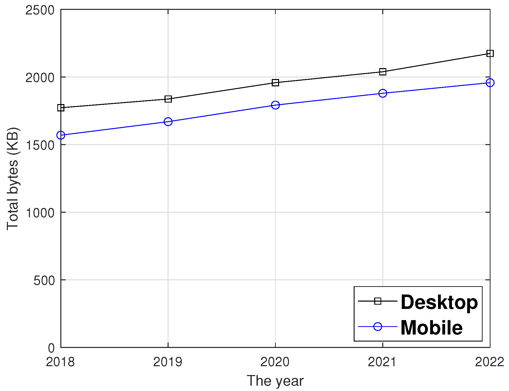Wired networks such as Gigabit Ethernet support throughput of tens of Gbps, while data rates of up to several Gbps are available in wireless networks such as 5G and WiFi 6 [1,2,3]. 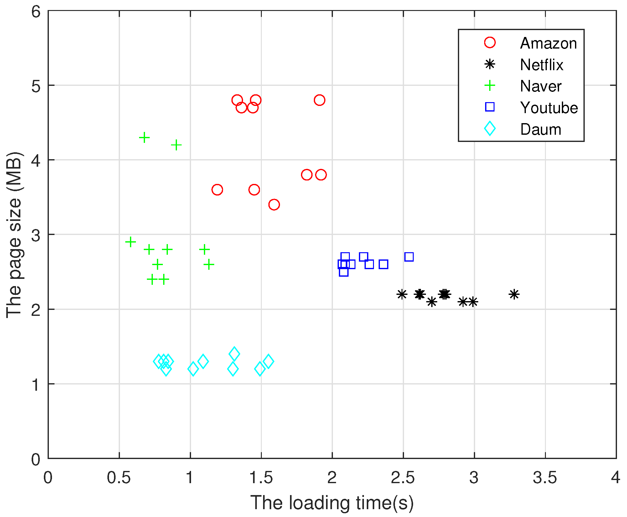With increasing network capability, the total bytes in a web page is also increasing, as shown in Figure 1 [4]. The web data have increased by more than 20% in desktop and mobile environments, from 1772 and 1569 KB in 2018 to 2174 and 1957 KB in 2022, respectively. However, the reduction in transmission latency is negligible, despite the median size of a web page being roughly 2.2 MB, which is trivial in comparison to network capacity. We utilized Pingdom to analyze the web data size and page load time of the Amazon, Netflix, YouTube, Naver, and Daum sites [5], and found that the average web page sizes are 4.2 MB, 2.1 MB, 2.6 MB, 2.9 MB, and 1.2 MB, and the average loading times are 1.547, 2.798, 2.219, 0.824, and 1.102 seconds, respectively, as shown in Figure 2. The result indicates that the transmission delay is significant in comparison to the network capacity of Gbps.

Figure 1. Median web page size.

Figure 2. Loading time and size of web pages.

Furthermore, 5G and WiFi 6 have been prepared to support low-latency communication [6,7,8,9]. In 5G, the 3GPP establishes three visions: enhanced mobile broadband (EMB), massive machine-type communications (MMTC), and ultra-reliable and low-latency communication (URLLC). Among them, URLLC aims for a delay time of less than 1 ms and transmission reliability of 99.99 % in radio access networks to meet the demand for low-latency communication [6,7]. In WiFi 6, several methods such as orthogonal frequency division multiple access (OFDMA) and spatial reuse (SR) have been proposed to improve user performance metrics such as reduced latency in heavily crowded areas [8,9].

Studies on the low-latency transmission of web content in transport and application layers have proposed using SPDY and Quick UDP Internet Connection (QUIC) protocols [10]. SPDY, an application layer protocol, uses multiplexing, header compression, and server push to minimize the web page load time [11]. The proposed features were included in the HTTP/2 standard, but SPDY support was phased out in 2016. The QUIC protocol is a novel transport layer protocol recently standardized by the Internet engineering task force (IETF) [12,13,14]. For reduced transmission latency, QUIC employs 0-RTT to reduce the connection establishment time, multiple streams within a connection to avoid head of line (LOL) blocking from sequential TCP delivery, and a new packet number to eliminate retransmission ambiguity. Hence, for network-based services demanding an immediate response, the QUIC protocol is often used to provide low-latency service.

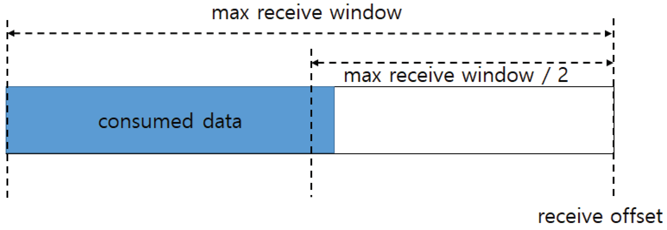
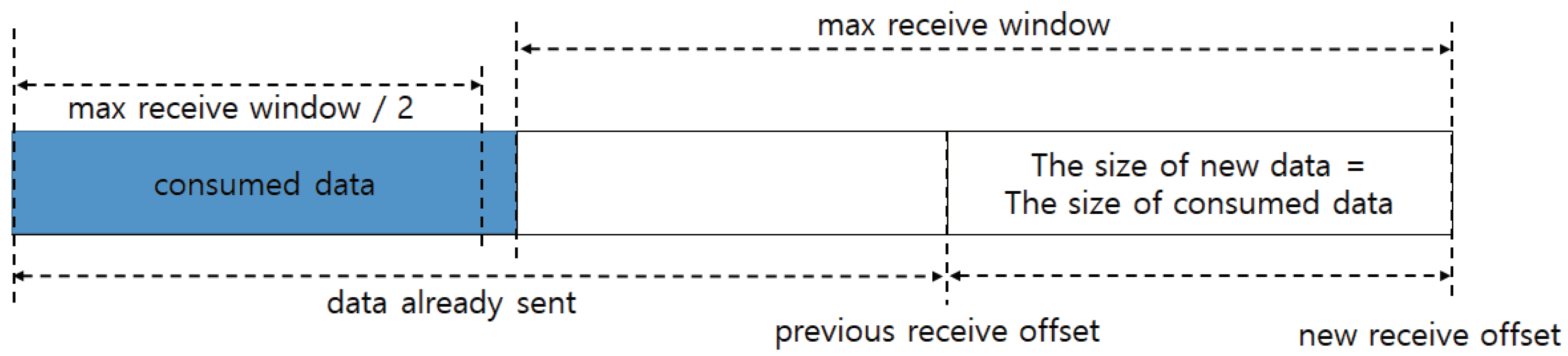
Flow control is disabled in TCP, because the buffer size is sufficiently large to accommodate the network-based service; moreover, packet errors caused by flow control are rare. However, the QUIC protocol allows for flow control to avoid buffer overflow, and employs static or autotuning allowances for flow control [15]. The static allowance employs a fixed-size maximum receive window [16]. The sender delivers data within the maximum receive window to avoid buffer overflow. The receiver notifies the sender of a receive window update by sending the MAX_STREAM_DATA frame when the upper layer protocol has read more than half of the maximum receive window, as shown in Figure 3. Because the amount of remaining data in the receive window is not half, the receive window is not updated until new data arrive. After one RTT, the receiver receives new data, and half of the maximum receive window is then updated. This indicates that the sender can only transmit half of the receive window at each RTT [17]. Google proposed autotuning allowance [16]. The maximum receive window size is doubled if the receive window update period is shorter than a threshold. Moreover, the receive window is no longer increased after reaching the upper limit or the update cycle has stabilized. In contrast, autotuning requires time to find a suitable receive window size. Therefore, reducing the maximum receive window search time is important for low-latency transmission.

Figure 3. Transmission condition of MAX_STREAM_DATA frame.

In this paper, we propose a fast autotuning scheme for low-latency transmission. The increase factor in fast autotuning is determined to be inversely proportional to the receive buffer occupancy. If the buffer occupancy is low, the increase factor is increased. Otherwise, the increase factor has been set to a low value. By rapidly widening the receive window while avoiding buffer overflow, the suggested approach can decrease transmission latency. We used the ns-3 simulator for performance evaluation [18]. Fast autotuning reduced transmission delays by 29% and increased throughput by 12% compared to autotuning in simulations employing a large buffer.

The rest of this paper is organized as follows: We present related works along with the motivation of this work in Section 2. The proposed fast autotuning method is detailed in Section 3. In Section 4, we evaluate fast autotuning allowance based on extensive simulations. Finally, the conclusions are presented in Section 5.

2. Related Works

The QUIC protocol suggests many approaches for reducing the web application data transmission time [12,13,14]. To decrease the connection establishment time, QUIC employs two methods: 1-RTT and 0-RTT handshakes for the initial and reestablishment connections, respectively. When the client connects to the server for the first time, QUIC performs a 1-RTT handshake and exchanges data transmission information such as the maximum receive window for flow control. The 0-RTT handshake shortens the connection establishment when the client reestablishes the connection with the server. Additionally, QUIC uses stream multiplexing to avoid HOL blocking in a connection. When one stream experiences a transmission delay due to HOL, the other streams continue to transmit data normally, and minimize delay.

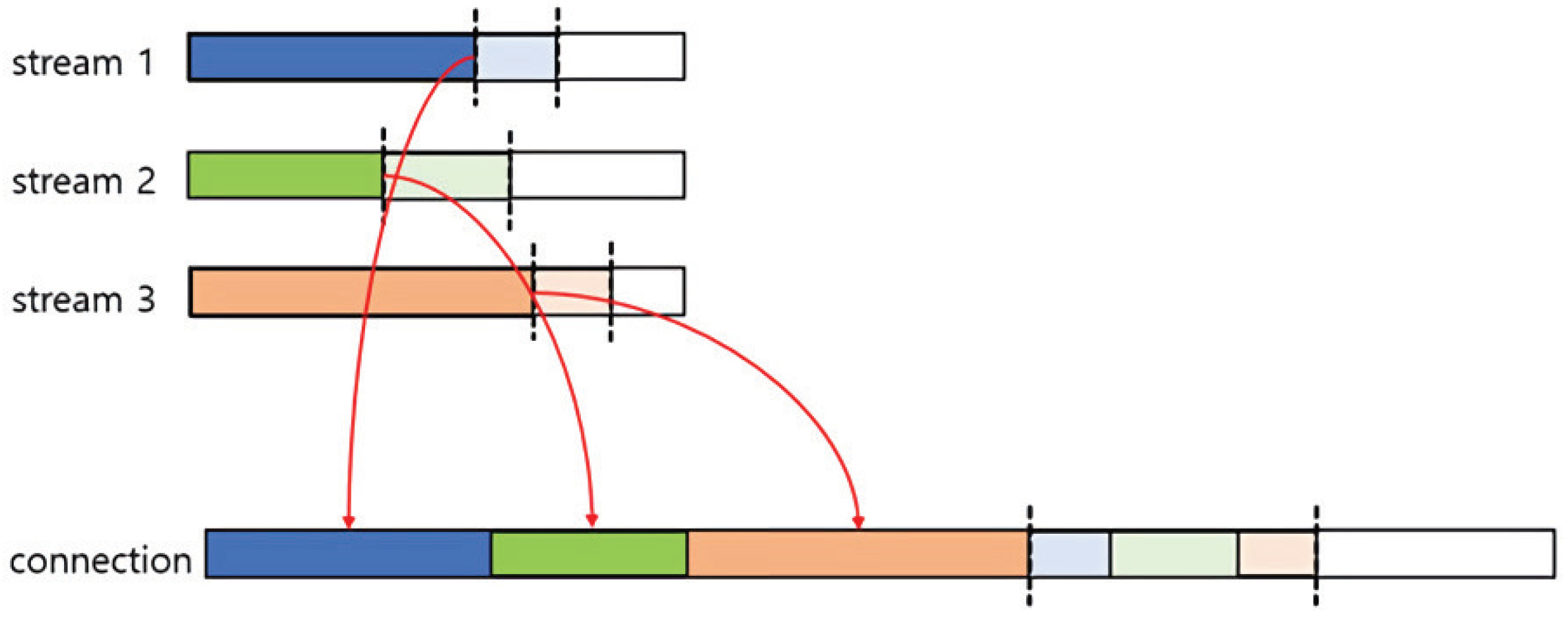
The QUIC protocol also uses flow control that limits bytes sent on a stream and connection to prevent buffer overflow. The maximum amount of transmission in a stream and connection is advertised during the 1-RTT handshake. A receiver sends the MAX_STREAM_DATA or MAX_DATA frame to advertise the new limit of the buffer. The MAX_STREAM_DATA frame represents one stream’s maximum transmission byte offset. If the sender has sent the maximum bytes in a stream, the transmission is blocked until the sender receives a MAX_STREAM_DATA frame from the receiver. The MAX_DATA frame represents the maximum transmission byte offset of the connection, equivalent to the total of all streams’ maximum transmission byte offsets, as shown in Figure 4.

Figure 4. Connection-level flow control.

Google QUIC has proposed a static allowance for flow control [16]. The receive window in a static allowance is allocated a fixed amount of memory. As shown in Figure 3, the receiver transmits the MAX_STREAM_DATA frame if the consumed data, which are data read from the upper layer, exceed half of the maximum receive window. 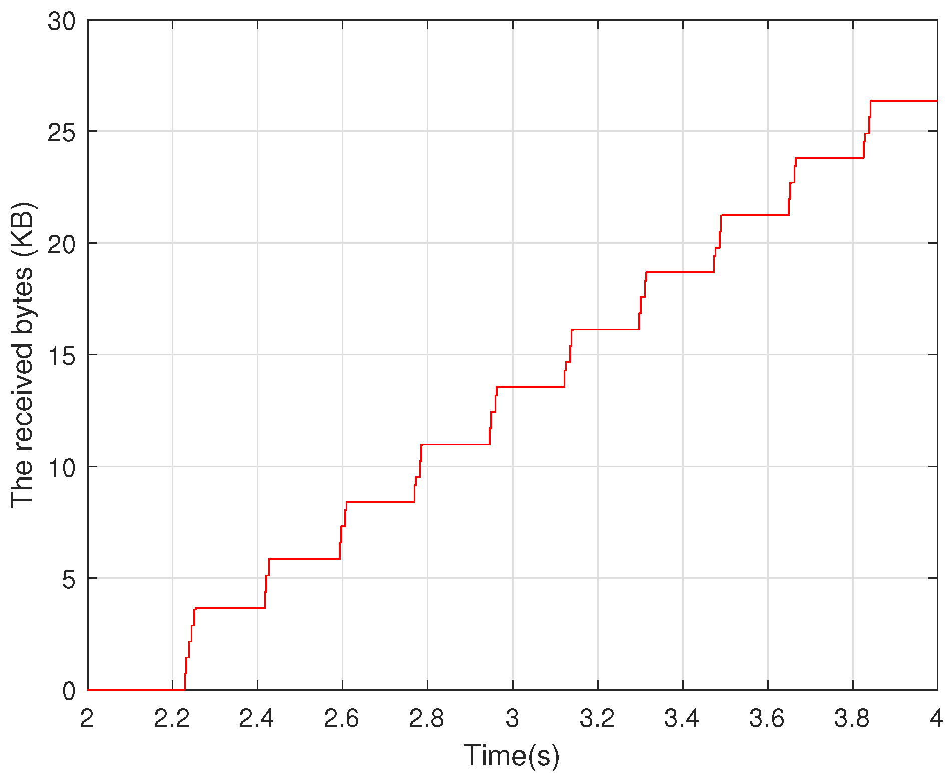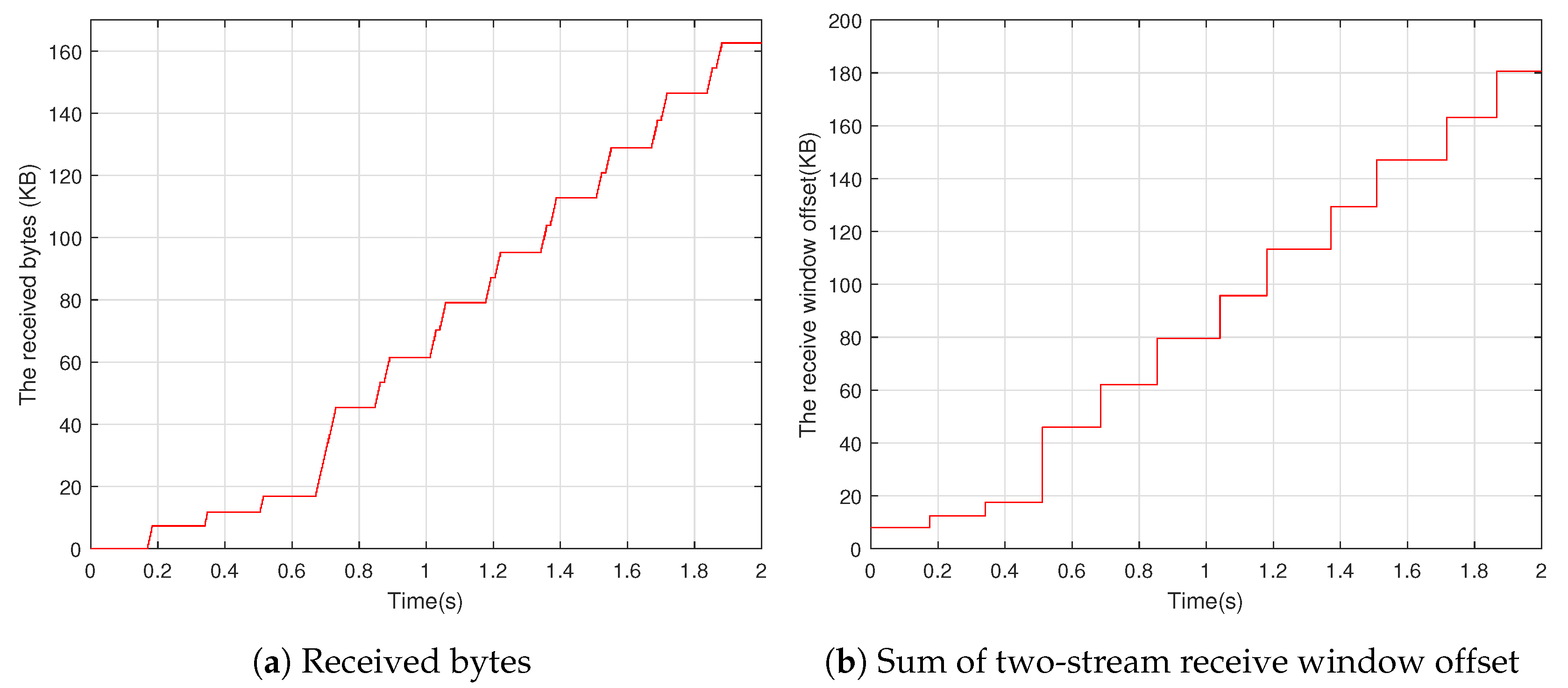The receive offset grows by the maximum receive window from the consumed data after receiving the MAX_STREAM_DATA frame from the sender, as shown in Figure 5. However, the sender can only transmit data equivalent to around half of the maximum receive window since the data have already been transferred in the previous transmission. After transmitting the MAX_STREAM_DATA frame, the receiver does not send the MAX_STREAM_DATA frame until new data arrive because the remaining receiver data size is less than half of the maximum receive window. The bytes received by a stream with a static allowance when two streams are transmitted in the ns-3 simulator are depicted in Figure 6. The stream has 4 KB of the maximum receive window. After the initial data, the receiver receives around 2.5 KB of data on average every RTT, indicating that the sender uses half of the receive window to transmit data.

Figure 5. Increased receive offset by receiving MAX_STREAM_DATA frame.

Figure 6. Received bytes of a stream with static allowance.

In [17], the improved static allowance scheme was proposed to solve the throughput degradation in static allowance. The receiver transmits a MAX_STREAM_DATA frame if the amount of consumed data is larger than (threshold-MSS). Half of the maximum receive window is used as the threshold, and MSS is the maximum segment size. In other words, the MAX_STREAM_DATA frame is sent one packet earlier than the static allowance. The receive window updates occur twice within one RTT because the remaining data exceed (threshold-MSS). Thus, the sender transmits as many data as the maximum receive window allows in every RTT. Google has proposed autotuning allowance to search for an appropriate receive window [16]. If the time interval between two MAX_STREAM_DATA frames is less than twice the RTT, the current receive window is identified as insufficient, and the maximum receive window is doubled. Moreover, an upper bound prevents indefinite increments in the receive window.

Compared to prior works, the proposed scheme aims to reduce the transmission delay caused by flow control. The improved static allowance uses the allocated receive window fully. However, if the maximum receive window is smaller than the transmission rate, the transmission is delayed until the MAX_STREAM_DATA frame is received, because the improved static allowance also utilizes a fixed memory size. The autotuning allowance increases the receive window size to prevent transmission interruption. However, to determine an adequate maximum receive window, the autotuning allowance requires several RTTs, increasing the transmission latency. Moreover, for small data sizes, an adequate receive window will not be identified until transmission completion. The proposed fast autotuning allowance reduces the search time for finding an adequate receive window. The receiver increases the receive window exponentially if free buffer space is sufficient; otherwise, the receive window is not enlarged to avoid buffer overflow. The computational overhead is minimal because of the low complexity of the proposed algorithm.

3. Proposed Scheme

This section details the proposed fast autotuning allowance strategy. We first present the calculation of the buffer occupancy, based on which an increase factor is determined. At time t, the buffer occupancy of a stream, $B_{str}\left(t\right)$, is expressed as Equation (1). $S_{upper}$ and $S_{win}$ are the upper bound and the current maximum receive window of the stream, respectively.

$$B_{str}\left(t\right)=\frac{S_{win}}{S_{upper}}\times 100$$

(1)

In the QUIC protocol, because a sender or a receiver can generate a stream if necessary, buffer occupancy calculations are required for both streams and connections. For a connection at time t, the buffer occupancy of a connection, $B_{con}\left(t\right)$, is calculated using Equation (2). $C_{upper}$ is the upper bound of the buffer for a connection. The increase factor is determined based on the buffer occupancy after a receive window update.

$$B_{con}\left(t\right)=\frac{\sum S_{win}}{C_{upper}}\times 100$$

(2)

The fast autotuning algorithm is described in Algorithm 1. By subtracting consumed bytes, $C_{bytes}$, from maximum receive window offset, $W_{maxoffset}$, the receiver calculates the available receive window, $W_{avail}$. The receive window update is triggered if the available receive window is less than $W_{max}/2$; the receiver then delivers the MAX_STREAM_DATA frame for a stream (or MAX_DATA frame for a connection). $F_{inc}$, the increase factor, is determined based on the buffer occupancy, if $T_{interval}$, the time since the last window update, is less than 2RTT. The buffer occupancy is calculated using Equation (1) for the stream and Equation (2) for the connection. Because sufficient free buffer space is not available if the buffer occupancy is greater than 75%, the increase factor is set to 2. The increase factor is set to 4 if the buffer occupancy is between 50 and 75%, it is 8 if the occupancy is greater than 25% but less than 50%, and it is 16 if the free buffer space exceeds 75%. The maximum receive window is then determined by the smaller of ($W_{max}\ast F_{inc}$) and $B_{upper}$, the upper bound of the buffer. The maximum offset of the receive window is increased by ($W_{max}-W_{avail}$), as depicted Figure 5. The fast autotuning seeks to reach the maximum receive window as quickly as possible. As a result, since the autotuning allowance doubles the maximum receive window, the increase factor in Algorithm 1 increases by the power of 2 based on the buffer occupancy. The autotuning, for example, requires two buffer updates to raise the maximum receive window by four times, but the fast autotuning only requires one.

Algorithm 1 Fast autotuning

1: $W_{avail}=W_{maxoffset}-C_{bytes}$  2:    3: if$W_{avail}<W_{max}/2$then  4:        if $T_{interval}<RTT\ast 2$ then  5:              if $B_{occupancy}>=75$ then  6:                     $F_{inc}=2$  7:              else if $50<=B_{occupancy}<75$ then  8:                     $F_{inc}=4$  9:              else if $25<=B_{occupancy}<50$ then 10:                     $F_{inc}=8$ 11:             else if $B_{occupancy}<25$ then 12:                     $F_{inc}=16$ 13:             end if 14:   15:             $W_{max}=min(W_{max}\ast F_{inc},B_{upper})$ 16:        end if 17:   18:        $W_{maxoffset}+=(W_{max}-W_{avail})$ 19:        send MAX_STREAM_DATA (or MAX_DATA) 20: end if

For example, a sender uses a QUIC connection with one stream to transfer data to a receiver. The upper bounds for the stream and the connection are 128 KB and 256 KB, respectively. The stream’s and connection’s initial maximum receive windows are 4 KB and 8 KB, respectively. Because the buffer occupancy is less than 25% of the stream upper bound when the first buffer update occurs, the increase factor is set to 16 and the maximum receive window is set to 64 KB. Because the buffer occupancy is 50%, the increase factor for the second buffer update is calculated to be 4. The maximum receive window, on the other hand, is set to 128 KB because the stream upper bound cannot be exceeded.

We implemented three flow control algorithms: static, autotuning, and fast autotuning allowances. First, we analyzed the ns-3 simulator with QUIC [19], and then modified four classes: QuicL5Protocol, QuicSocketBase, QuicStreamBase, and QuicStreamRxBuffer classes. For example, Algorithm 1 should determine the available amount of data for a stream or connection. We modified AvailableWindow function in the QuicSocketBase class to calculate the available amount of data by subtracting CalculateAllRecv() from the m_max_data variable. In the function, m_max_data variable means the maximum amount of data that can be sent on the connection and CalculatedAllRecv() in the QuicL5Protocol class indicates the amount of received data.

4. Evaluation

We evaluate the performance of the fast autotuning allowance using an ns-3 simulator [18], and compare the results to the static and autotuning allowances [15,16]. In [15], the static allowance is utilized in seven out of ten representative IETF QUIC implementations, while the autotuning allowance, which is used in quiche, is a flow control mechanism proposed by Google recently. As discussed earlier, we implemented static, autotuning, and fast autotuning allowance in the ns-3 simulator and measured the throughput and transmission time for performance evaluation. We measured the bytes received by the receiver with a tiny buffer for each of the three flow control models. Then, we extended the experiment to evaluate the performance of a four-stream connection with a large buffer. Finally, the transmission delay for each data size was measured through simulations.

4.1. Two-Stream Connection with Small Buffer

We simulated and measured the throughput of a connection with static, autotuning, and fast autotuning allowances. The number of streams, the maximum receive window, and the upper bound are listed in Table 1. First, we evaluated the throughput of a two-stream connection with static allowance. The average throughput was 234.56 Kbps, and Figure 7a depicts the bytes received by the receiver over time. Because the sum of the maximum stream receive window was 8 KB, approximately 7.32 KB of data were sent in the initial transmission. Since the buffer update occurs when the consumed bytes exceed half of the receive window (Figure 7b), approximately 4.3 KB to 5.1 KB of data were transferred in the second transmission.

Table 1. Parameter setting for a two-stream connection.

Parameters	Value
Number of streams	2
Maximum connection receive window	8 KB
Maximum stream receive window	4 KB
Connection upper bound	64 KB
Stream upper bound	16 KB

Figure 7. Static allowance in a two-stream connection with small buffer.

In a two-stream connection with autotuning allowance (Figure 8), the sender sends 4.39 KB and 5.12 KB of data after the first and second buffer updates, respectively, and the receive window is kept at 8 KB, as with the static allowance. The receive window grows to 16 KB when the third buffer update happens at around 0.5 s. The receive window offset rises by around 12.39 KB, with 4.39 KB of consumed bytes (half of the previous receive window) and 8 KB of a new receive window increment. When the fourth buffer update happens at 0.68 s, because the receive window abruptly increases to 24 KB instead of 32 KB, the sender transmits 16.35 KB (8.35 KB for consumed bytes and 8 KB for increment). This is because one of two streams extends the receive window to 16 KB, while the other maintains an 8 KB receive window. The receive window of the stream with the 8 KB window grows to 16 KB in the fifth buffer update, and the aggregate grows to 32 KB. The sum of the streams’ receive windows is kept at 32 KB.

Figure 8. Autotuning allowance in a two-stream connection with small buffer.

Figure 9 shows the simulation results for fast autotuning allowance. Fast autotuning achieves approximately 7% of throughput gain compared to autotuning (Figure 9a). The throughput gain by fast autotuning is achieved by rapid growth of the receive window. During the two buffer updates, the aggregate of the receive windows of two streams is maintained at 8 KB. The receive window is extended by four times to 32 KB after the third buffer update in 0.5 s. Because a stream’s receiver window is 4 KB and the stream upper bound is 16 KB, the increase factor is 8. $W_{max}\ast F_{inc}$ is 32 KB, but $W_{max}$ is calculated as 16 KB because the stream upper bound is 16 KB. Because the aggregate receive window is 32 KB, 28.39 KB of data (24 KB for new increment and 4.39 KB for consumed bytes) are transmitted, and fast autotuning maintains the aggregate receive window at 32 KB.

Figure 9. Fast autotuning allowance in a two-stream connection with small buffer.

4.2. Four-Stream Connection with Large Buffer

We evaluated the performance for a four-stream connection with a large buffer. The parameter settings are listed in Table 2. The initial maximum stream receive window was 8 KB and the upper bound of a stream was 1 MB. The received bytes over time for autotuning and fast autotuning allowance in Figure 10 show average throughputs of 4.8 and 5.4 MB per second, respectively. Compared to autotuning allowance, fast autotuning allowance increases throughput by 12.5% because it increases the maximum receive window significantly. Figure 11 depicts the maximum receive window for one stream with autotuning and fast autotuning. In autotuning, the maximum stream receive window is doubled from 8 KB to 512 KB for 2.5 s, and then maintained at 512 KB. However, in fast autotuning, the maximum stream receive window grows 16 times in 0.86 s, from 8 KB to 128 KB, and then four times in 1.03 s, from 128 KB to 512 KB, which is 1.5 s faster than autotuning.

Table 2. Parameter setting for a four-stream connection.

Parameters	Value
Number of streams	4
Maximum connection receive window	32 KB
Maximum stream receive window	8 KB
Connection upper bound	64 MB
Stream upper bound	1 MB

Figure 10. Received bytes of a connection with large buffer.

Figure 11. Maximum stream receive window.

We also measured the transmission latency for each data size. Compared to autotuning, fast autotuning reduces transmission latency by around 29% on average (Figure 12). The transmission latency is decreased by at least 30% when transmitting 1 MB to 5 MB data, the average data size communicated over the Internet.

Figure 12. Transmission time by data size.

5. Conclusions

We proposed a fast autotuning allowance to reduce transmission latency by rapidly increasing the maximum receive window based on the buffer status. If the available buffer is large, the receive window is rapidly increased to decrease transmission latency. The simulation results showed that the proposed scheme can increase the performance improvement in network scenarios. We plan to look into the settings for parameters such as the buffer occupancy and the increase factor in the future.