Article

A Grey-System Theory Approach to Assess the Safety of Gas-Supply Systems

by
Dawid Szpak
1,
Barbara Tchórzewska-Cieślak
1,
Katarzyna Pietrucha-Urbanik
1,* and
Mohamed Eid
2
1
Department of Water Supply and Sewerage Systems, Faculty of Civil, Environmental Engineering and Architecture, Rzeszow University of Technology, Al. Powstancow Warszawy 6, 35-959 Rzeszow, Poland
2
National Institute of Applied Sciences of Rouen-LMN, INSA-Rouen, 685 Avenue de l’Université-BP 08, 76801 St. Etienne du Rouvray, France
*
Author to whom correspondence should be addressed.
Energies 2022, 15(12), 4240; https://doi.org/10.3390/en15124240
Submission received: 8 March 2022 / Revised: 28 May 2022 / Accepted: 7 June 2022 / Published: 9 June 2022

Abstract

:
The continuity of gas-supply service is a major concern for all gas-supply operators. A safety review of a gas-supply system could help to mitigate the potential repercussions of supply disruptions. Disruptions occur at random due to systemic failures in gas distribution networks. Assessing the operational safety of gas distribution networks is challenging and complex, especially when operational data are limited or associated with high uncertainty. This paper focuses on gas leak incidents. Natural gas leaks disrupt the production process and endanger the ecosystem. Mechanically originated damage in pipelines is found to be the major cause of leaks, according to our investigations. This paper proposes a three-parameter risk matrix to be used in the safety analysis of gas-supply systems. This paper then raises the possibility of using grey-system theory. Grey-system theory has been used to overcome the limitations of the conventional matrix method. This choice is motivated by two facts: our data are heterogeneous with a high level of uncertainty, and some of the data are based on experts’ judgement and maintenance reports using qualitative metrics. It is underlined how GST provides insight for the decision-making process, even in the absence of complete information sets. The method developed here is advocated in the context of procedures ensuring the safety and the supply continuity of gas-supply systems.

1. Introduction

The US Department of Transportation finds that pipeline safety as a trend has showed a steady decrease in numbers of incidents giving rise to death and injury over the last twenty years—from around 60 a year in the 1990s down to 40 or so in the present day (2020). Interest in renewal is high, as more than 50% of the length of the gas network was installed between the 1950s and the 1960s. Many programs to address and improve the situation have been launched in order to reduce failure due to the occurrence of different failure modes throughout the gas distribution network [1,2].
For gas-supply operators, the evaluation of the frequency of failure occurrence is an important concern. It is of even greater concern when it is a matter of designing gas-supply systems [3,4] with new technology. Equally, even when we leave aside the direct safety aspects, the increased pressure from environmentalists and stricter standards are pushing for the development and implementation of advanced safety assessments [5].
On this basis, renovation or modernisation of gas distribution networks requires the assessment and classification of the state of the pipelines, as well as the determination of required repair actions, and their criticality [6,7,8]. Hence, the preventive maintenance through repair, renovation and replacement decisions becomes rational. Rational preventive maintenance decreases the occurrence likelihood of potential failures, [9]. Subsequently, it reduces the risk of supply disruptions [10,11], as is true for all other industrial- and service-supply sectors. Less frequent pipe-failures and disruptions in supply distribution obviously improves the profitability of the supply process, [12,13,14].
This work’s main objective is to develop a safety analysis of gas-supply systems using a synthetic risk matrix based on grey-system theory (GST). GST is gaining wide interest in a variety of fields [15]. Grey-system theory has been used to overcome the limitations of the conventional matrix method. The grey-system theory approach focuses on reducing the contribution of the epistemological errors in probabilistic risk analyses and assessments by the integration of uncertainties and their distributions. It increases, then, the robustness of safety assessments.
Real data on gas-supply network failures were used to conduct the analysis. Real data are available through technical reports and information gathered during daily operations. Data are controlled by the municipality gas utilities in Poland.
Overall, this article outlines current gas-supply safety requirements while also proposing a novel approach to risk analysis in gas-supply systems.

2. The Approach

2.1. The Risk Matrix

The three-parameter risk formula has the following form:
r = P · F · N C
wherein P is a point weight of the occurrence of a specific failure mode, F is a point weight of that specific failure mode within all other possible failure modes in the system (in accordance with Equation (2)), and NC is a point weight of the consequent hazards associated to that specific failure mode.
Random systemic events, human actions, extreme operational conditions, system age, and environmental factors could all cause system failures.
A failure occurrence rate λ is calculated using the following equation:
λ = n ( Δ t ) Δ L · Δ t
where nt) represents the number of failures observed during the time duration Δt and along a pipe of length ΔL.
The involved parameters (Equation (1)) are allocated point-weighting figures, according to a scale defined in the risk matrix approach (a ten-point scale was adopted) [16,17,18,19].
Individual parameters, on the other hand, are given membership function parameters in accordance with a points scale, as follows (Figure 1):
  • negligible (0,0,1,2),
  • low (1,2,3,4),
  • medium (3,4,6,7),
  • high (6,7,8,9),
  • very high (8,9,10,10).
Each individual membership function i is bounded by a lower boundary a i and an upper boundary b i , i [ 1 , 2 , 3 , 4 , 5 ] . The global interval of the five functions is bounded by a lower boundary c = 0 and an upper boundary b = 10 . Then, each membership function i is defined by 4 points ( a i , b i 1 , a i + 1 , b i ), as follows (Figure 1).
It was also suggested to distinguish between five supply disruption phases according to the daily supply disruption interval T d :
  • T d = 0 : no gas supply disruption,
  • 0 < T d 4   h : short disruption,
  • 4   h < T d 8   h : medium disruption,
  • 8   h < T d 12   h : long disruption,
  • T d > 12   h : critical disruption.
The period during which a gas supply is unavailable is defined as the time during which a group of consumers is unable to use this source of energy, i.e., from the time of failure until the repair is completed and the gas supply is restored. Consumers’ dissatisfaction is proportional to the duration of the supply disruption, and certainly not in a linear pattern. In extreme situations, such a scenario may progress beyond the level of “critical” to the level of “crisis”, especially during winter season. The authors established the criteria based on their own research and analysis of the topic in the literature. The criteria could be customized to fit the specificity of a different gas-supply network.
Individual parameters are then established using the following criteria:
  • The weight scale of a given type of failure mode (P):
    P 0.1 , negligible,
    0.1 < P 0.2 , low,
    0.2 < P 0.4 , medium,
    0.4 < P 0.6 , high,
    P > 0.6 , very high.
  • The weight scale (F) according the annual-longitudinal rate of failure λ along the gas-supply network:
    λ 0.05   km 1 · y 1 , negligible,
    0.05 < λ 0.10   km 1 · y 1 , low,
    0.1 < λ 0.3   km 1 · y 1 , medium,
    0.3 < λ 0.5   km 1 · y 1 , high,
    λ > 0.5   km 1 · y 1 , very high.
  • Supply disruption criticality level (NC) as a function of the disruption duration:
    T d = 0 , negligible,
    0 < T d 4   h , low,
    4   h < T d 8   h , medium,
    8   h < T d 12   h , high,
    T d > 12   h , very high.

2.2. Grey-System Theory

The matrix proposed is, in fact, based on strictly defined numerical values, so that the aspect of subjectivity in the analysis is reduced (Section 2.1) and allows better integration of the epistemological uncertainty.
Given the constraints of the traditional risk matrix method, it was recommended that this be modified to incorporate the theory of grey systems as described by J.L. Deng [20]. This can be used to examine the operation of (so-called grey) systems with limited or imprecise databases, i.e., associated with higher levels of uncertainties. Considering the limitations in modelling pipe-failures and the complexity of the interactions between different parameters (causes, mechanisms, modes, criticality, and effects), the entire supply network can be considered as a complicated grey system in practice. White systems are those in which all parameters are fully known and can be well-described by classical applied statistics. Hence, the added value of the theory of grey systems is in allowing decisions to be made in the absence of fully comprehensive data sets and admitting the systematic subjectivity of expert judgments. It is especially significant in the case of a gas-supply system if the company does not keep records of undesired events of certain types, or if a hypothetical event has not happened yet, but its future occurrence can obviously be expected.
Other critical infrastructures, e.g., water supply systems, have already applied GST [21].
As shown in Figure 1, the work to analyse the P, F, and NC input parameters adapts trapezoidal and triangular membership functions, in line with the short number of data required to identify the function and the opportunity to change function parameters during the research.
The selection of an appropriate membership function is a critical step in the created approach for analysing the occurrence of failures, and it has a substantial effect on the analyses’ outcomes. Linguistically, these parameters are classified in terms of their being low, medium, or high. Thus, in this scenario, set boundaries are clearly specified, and a progressive transition from lack of membership to complete membership of a particular element in the set occurs. Because the employment of grey-systems theory in the study of failure mode and the impact of failure improves analysis efficiency [22,23], its implementation in a matrix approach is likely to mitigate the method’s drawbacks.
Sharp values are determined in accordance with the relationship proposed in the literature [24] once each parameter characterizing an undesired event has been assigned a matching linguistic variable.
Let n be the number of member functions we have (n = 5) as shown in Figure 1. Each member function is bounded by a lower bound ( a i ) and a higher bound ( b i ). The lowest bound of all the boundaries is c ( c = 0 ) and the highest of all is d ( d   = 10).
The matching factor of each function K ( i ) is determined by:
  K ( i ) = ( b i c ) + ( a i + 1 c ) [ ( b i c ) + ( a i + 1 c ) ] [ ( a i d ) + ( b i 1 d ) ]
where i     [ 1 ,   2 ,   3 ,   4 ,   5 ] assigns five qualitative members, b j < 1 = c = 0 , a j > 5 = d = 10 as members (0) and (6) do not exist.
Accordingly, one can determine the matching factors as following:
  • negligible: (i = 1)
K ( 1 ) = ( b 1 c ) + ( a 2 c ) [ ( b 1 c ) + ( a 2 c ) ] [ ( a 1 d ) + ( b 0 d ) ] = [ 2 + 1 ] [ 3 ] [ ( 0 10 ) + ( 0 10 ) ] = 0.13 ,
  • low: (i = 2)
K ( 2 ) = ( b 2 c ) + ( a 3 c ) [ ( b 2 c ) + ( a 3 c ) ] [ ( a 2 d ) + ( b 1 d ) ] = [ 4 + 3 ] [ 7 ] [ ( 1 10 ) + ( 2 10 ) ] = 0.29 ,
  • medium: (i = 3)
K ( 3 ) = ( b 3 c ) + ( a 4 c ) [ ( b 3 c ) + ( a 4 c ) ] [ ( a 3 d ) + ( b 2 d ) ] = [ 7 + 6 ] [ 13 ] [ ( 3 10 ) + ( 4 10 ) ] = 0.50 ,
  • high: (i = 4)
K ( 4 ) = ( b 4 c ) + ( a 5 c ) [ ( b 4 c ) + ( a 5 c ) ] [ ( a 4 d ) + ( b 3 d ) ] = [ 9 + 8 ] [ 17 ] [ ( 6 10 ) + ( 7 10 ) ] = 0.71 ,
  • very high: (i = 5)
K ( 5 ) = ( b 5 c ) + ( a 6 c ) [ ( b 5 c ) + ( a 6 c ) ] [ ( a 5 d ) + ( b 4 d ) ] = [ 10 + 10 ] [ 20 ] [ ( 8 10 ) + ( 9 10 ) ] = 0.87 .
The values of c for the beginning of the range equal to 0 and d for the end of the compartment equals 3 are constant for all the linguistic variables, with values a0 and b0 relating to boundaries for each linguistic variable, the membership function being 0, while a1 and b1 are determined for the boundaries of individual variables, where the membership function is 1.
A n-element comparative series can be written as:
x i = ( x i ( 1 ) ,   x i ( 2 ) , , x i ( k ) ) X
where x i   refers to the k-th indicator xi.
If all the series are equivalent, the matrix [21] can be used to illustrate them:
x = [ x 1 ( 1 )     x 1 ( 2 )       x 1 ( 3 ) x 2 ( 1 )     x 2 ( 2 )       x 2 ( 3 )                                 x n ( 1 )     x n ( 2 )       x n ( 3 ) ]
By calculating the optimum level of all the characteristics that affect the risk value, a standard set of choice factors is established. From the perspective of gas customers’ interests, the lowest attainable level of each individual characteristic should be maintained. As a result, the standard series can be presented in the following form:
x 0 = [ x 0 ( 1 ) ,   x 0 ( 2 ) ,   , x 0 ( k ) ] = [ low ,   low ,   low ]
These data are displayed as a matrix, just as the comparable series [23].
The following matrix depicts the differences between the comparative and standard series (after Pillay et al., 2003):
D 0 = [ Δ 01 ( 1 )       Δ 01 ( 2 )       Δ 01 ( 3 ) Δ 02 ( 1 )       Δ 02 ( 2 )       Δ 02 ( 3 )                                                   Δ 0 m ( 1 )       Δ 0 m ( 2 )       Δ 0 m ( 3 ) ]
where   Δ 0 j ( k ) = | x 0 ( k ) x i ( k ) | , x0(k) is the standard series, and xi(k) is the comparative series.
Formula is used to calculate the grey relation coefficient [25]:
γ ( x 0 ( k ) , x i ( k ) ) = min i min k | x 0 ( k ) x i ( k ) | + ζ max i max k | x 0 ( k ) x i ( k ) | | x 0 ( k ) x i ( k ) | + ζ max i max k | x 0 ( k ) x i ( k ) |
where ζ is the identifier; ζ     (0, 1).
To assess the degree of relatedness, the weighting coefficient values for parameters P, F, and NC should be chosen in such a way that the relationship is fulfilled:
k = 1 n β k = 1
Because the weighting factor is set by all team members involved in the study, the experts’ choices have a significant impact on the outcomes. The robustness of the choices depends on the extensive experts’ knowledge on both system functioning and risk-management strategies.
The degree of strength of the grey relation demonstrates the connection between possible causes and appropriate levels for decision-making elements [23]:
Γ ( x i , x j ) = k = 1 n β k γ { x i ( k ) , x j ( k ) }
As a result, the lower the risk of the given event occurrence, the higher the value determined from Equation (10). The degree of a relationship obtained can thus be referred to, as events are prioritised and areas in need of improvement are indicated.

3. Results

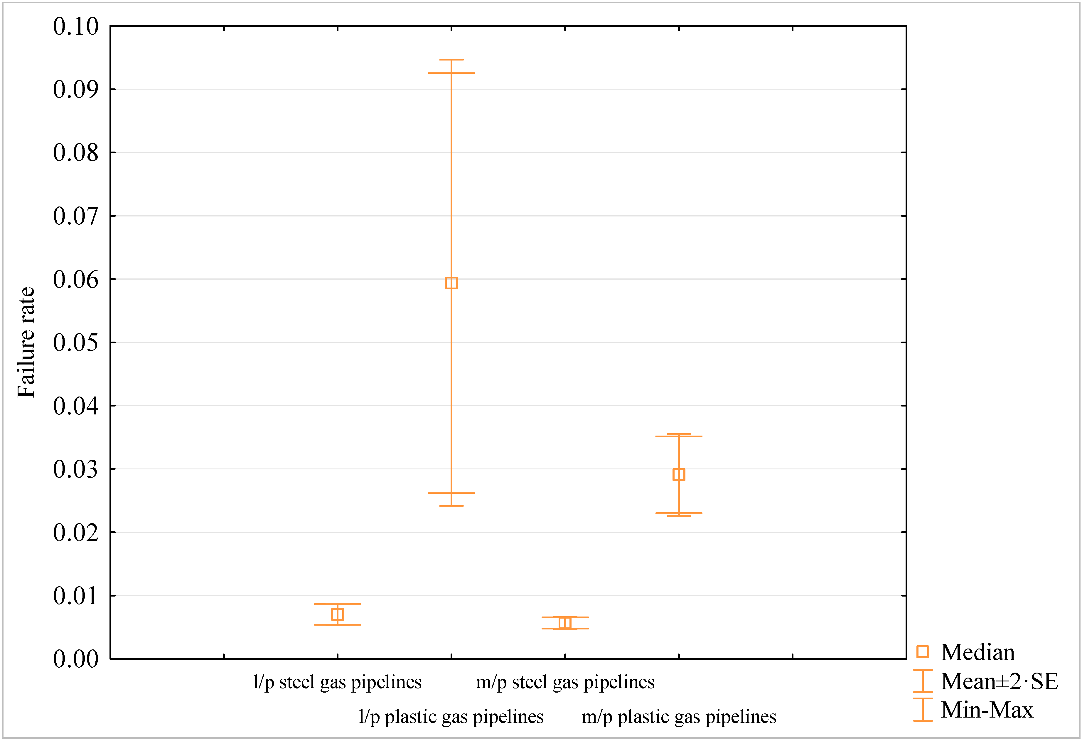
3.1. Analysing a Gas-Supply Network’s Technical State

The failure database developed by the gas-supply company—and made available to us—provides the basis for establishing a value of the network’s failure-rate index. This failure database encompassed dates and times of reporting; location of failure; date and time of the beginning and the end of the failure-rectification process; failure mode, causes and consequences; and the diameter and material of the pipes or other items used in treating the failure. The subsystem of natural-gas supply is supplied by a ring high-pressure network passing via first-order reduction and metering stations, with these supplying medium-pressure rings for the city’s different districts, as well as the neighbouring areas.
In Figure 2 and Figure 3, the network’s structure age and materials are depicted.
Figure 4 provides a graphic presentation of results for the analysis of causes of failure in the l/p (low-pressure) and m/p (medium-pressure) steel and plastic structures.
The failure rate index determined based on Formula (2) is presented in Figure 5.
The average value for the failure rate index was λav = 0.02555 failure/(km·year), assuming F = 1. We used the failure rate index limits indicated in [26,27,28,29] as reference thresholds in the absence of a standard value regulating the admissible limits. As the failure rate indices obtained in our case are lower than the reference thresholds, the studied gas-supply network can be considered in a good technical condition. This index has a considerable impact on gas customers’ perception of the service quality, as well as of the company’s trustworthiness and credibility.
The primary reasons for failures in the gas-supply network under analysis, as well as the average duration of the gas-supply disruptions, are listed in Table 1.
Table 1 offers the basis to draw the Pareto–Lorenz diagram [30] and to proceed on the assumption that a small number of causes explain most of the supply disruptions. This allows for the ranking of the disruption causes in terms of occurrence frequency and the identification of the areas that need corrective actions. Figure 6 shows the corresponding Pareto–Lorenz diagram indicating the causes of failures in the gas-supply network.
Table 1 offers the basis to draw the Pareto–Lorenz diagram [30], and to proceed on the assumption that a small number of causes explain most of the supply disruptions. This allows for the ranking of the disruption causes in terms of occurrence frequency and the identification of the areas that need corrective actions. Figure 6 shows the corresponding Pareto–Lorenz diagram indicating the causes of failures in the gas-supply network. The identified major disruption causes are the “mechanical damage”, “material wear”, and “defects in workmanship” that account for about 80% of all disruptions. To raise the level of reliability of the gas-supply network, measures should be taken to reduce the impact of the major causes. The other three minor causes were, in turn, responsible for just 20% of gas-supply disruption. Therefore, the assessment needs to consider not only the frequency of disruptions occurrence, but also their consequences (impacts). The assessment should equally be extended to encompass parameters associated with the disruption duration. Accordingly, short-term disruptions should be considered as reliability states not affecting the gas supply continuity.

3.2. Undesirable Events Prioritisation

After relationship (4), comparative series were created in the form of a matrix, using linguistic variables allocated to specific parameters which define each unwanted event. Another matrix was used to depict the standard series. The lowest level achievable by each input parameter is “low”, with the value of K(x) = 0.333 in this case. Then, in line with relationship (5), it is the comparative series vs. standard series that is determined [21].
x i = [ medium low medium medium low low medium low medium low low negligible negligible low medium negligible low low ] = [ 0.500 0.292 0.500 0.500 0.292 0.292 0.500 0.292 0.500 0.292 0.292 0.130 0.130 0.292 0.500 0.130 0.292 0.292 ]
x 0 = [ negligible negligible negligible negligible negligible negligible negligible negligible negligible negligible negligible negligible negligible negligible negligible negligible negligible negligible ] = [ 0.130 0.130 0.130 0.130 0.130 0.130 0.130 0.130 0.130 0.130 0.130 0.130 0.130 0.130 0.130 0.130 0.130 0.130 ]
D o = [ | 0.130 0.500 | | 0.130 0.292 | | 0.130 0.500 | | 0.130 0.500 | | 0.130 0.292 | | 0.130 0.292 | | 0.130 0.500 | | 0.130 0.292 | | 0.130 0.500 | | 0.130 0.292 | | 0.130 0.292 | | 0.130 0.130 | | 0.130 0.130 | | 0.130 0.292 | | 0.130 0.500 | | 0.130 0.130 | | 0.130 0.292 | | 0.130 0.292 | ] = [ 0.370 0.162 0.370 0.370 0.162 0.162 0.370 0.162 0.370 0.162 0.162 0   0   0.162 0.370 0   0.162 0.162 ]
The next step is to calculate a grey-relation coefficient for each variable in accordance with dependant relationship (6), which can be summarized as follows (following Deng 1982):
γ ( x 0 ( k ) , x i ( k ) ) = Δ min + ζ Δ max Δ 0 j ( k ) + ζ Δ max
where Δmin = 0, Δmax = 0.370, and ζ = 0.5.
Table 2 shows the results of the computations for the analysed unfavourable events. An example of the calculation for the event marked 2 in Table 2 would then be as follows:
γ P = 0 + 0.5 · 0.370 0.370 + 0.5 · 0.370 = 0.333 ,
γ F = 0 + 0 , 5 · 0.370 0.162 + 0.5 · 0.370 = 0.533 ,
γ N = 0 + 0 , 5 · 0.370 0.162 + 0.5 · 0.370 = 0.533 .
By giving suitable weights to the input parameters, the goal of the analysis is to identify locations that are particularly vulnerable to supply disruption causes. The repercussions or impact of the disruption causes, in this case, is understood in terms of the time over which gas distribution to consumers is withheld, which has the largest impact on the value for supply-service quality. The values for the weighing coefficient, as determined, were for parameter P—a weighting factor of 0.25, for parameter F—a weighting factor of 0.25, and for parameter NC—a weighting factor of 0.5.
The degree of the grey relationship identified in accordance with relation (9) for the occurrence marked 2 in Table 2 is as follows:
Γ ( x i , x j ) = 0.25 · 0.333 + 0.25 · 0.533 + 0.5 · 0.533 = 0.483 .
The lower the relationship’s intensity, the higher the impact on gas-supply continuity. Table 2 suggests that the greatest impact on gas-supply continuity is related to mechanical damage and defects in workmanship. Due to the relatively shallow foundation of gas pipes, the greatest risk is caused by accidental mechanical damage resulting from soil work and excavation. Therefore, final commissioning should be carried out with particular care, and any detected faults should be removed before the network is put into operation.

4. Conclusions

Realizing a risk assessment with input data of weak statistical quality is a real challenge. The authors propose an approach based on GST that factors in the experts’ judgements, and considers those judgements’ epistemological uncertainties. The approach works out some parameters amongst which the Γ factor is the most discriminant. The value of Γ allows for risk prioritization and comparisons between different gas-supply systems. Its value is not a direct representation of the risk, but it is an indicator whose value supports the ranking of undesired events, and so may indicate areas where corrective actions are required. This is unquestionably valuable information for a gas-supply operator. Major safety improvements are expected thanks to the assessment results and the exploitation of the developed approach.
In comparison with the conventional matrix method, the proposed method results in convergent and coherent results, as the most frequent failures result in the longest gas-supply disruption times. Conversely, prioritization based on the degree of relationship will produce different results if less-frequent failures have greater consequences. The analysis is carried out from the points of view of the consumers’ demand and the operators financial interest, for whom the mere fact of a failure is not significant, only the lack of gas supply is a concern.
It may be stated that the developed methodology enables the identification of the most critical failure modes. That can then be useful to build a modernization strategy for a given gas network. The proposed approach can be employed in various gas networks that lack the necessary IT resources. In such situations, it is helpful to associate the type of failure with gas-supply disruption events.
The assessment concluded that the longest disruption durations are caused by manufacturing defects, mechanical damage, and soil movement. If long-term gas -supply disruptions are to be reduced, special attention must be paid to the quality of the construction work, as well as to the protection of gas pipes from neighbouring construction and operation activities.
The life extension of existing gas-supply networks has continued to rise in recent years, resulting in an increase in the likelihood of gas network failures. Despite increased safety standards for network operation, different failure modes continue to be reported. That constitutes a real (even grave) threat to human health and life. As a result, advanced methods should be continually developed with the intention of reducing the likelihood of future pipeline failures.

Author Contributions

All authors equally contributed to the development of this manuscript. All authors have read and agreed to the published version of the manuscript.

Funding

This research received no external funding.

Institutional Review Board Statement

Not applicable.

Informed Consent Statement

Not applicable.

Data Availability Statement

Not applicable.

Conflicts of Interest

The authors declare no conflict of interest.

References

  1. Majid, Z.A.; Mohsin, R.; Yusof, M.Z. Experimental and computational failure analysis of natural gas pipe. Eng. Fail. Anal. 2012, 19, 32–42. [Google Scholar] [CrossRef]
  2. Shalaby, H.M.; Riad, W.T.; Alhazza, A.A.; Behbehani, M.H. Failure analysis of fuel supply pipeline. Eng. Fail. Anal. 2006, 13, 789–796. [Google Scholar] [CrossRef]
  3. Rafiq, M.; Akbar, A.; Maqbool, S.; Sokolová, M.; Haider, S.A.; Naz, S.; Danish, S.M. Corporate Risk Tolerance and Acceptability towards Sustainable Energy Transition. Energies 2022, 15, 459. [Google Scholar] [CrossRef]
  4. Mohsin, R.; Majid, Z.A. Erosive failure of natural gas pipes. J. Pipeline Syst. Eng. 2014, 5, 818–837. [Google Scholar] [CrossRef]
  5. Dieckhoener, C.; Lochner, S.; Lindenberger, D. Simulating the Effects of European Natural Gas Infrastructure Developments. Oil Gas-Eur. Mag. 2010, 36, 174–185. [Google Scholar]
  6. Ondrejka Harbulakova, V.; Estokova, A.; Kovalcikova, M. Correlation Analysis between Different Types of Corrosion of Concrete Containing Sulfate Resisting Cement. Environments 2017, 4, 44. [Google Scholar] [CrossRef]
  7. Szpak, D. Method for Determining the Probability of a Lack of Water Supply to Consumers. Energies 2020, 13, 5361. [Google Scholar] [CrossRef]
  8. Tchorzewska-Cieslak, B.; Boryczko, K.; Eid, M. Failure scenarios in water supply system by means of fault tree analysis. Adv. Saf. Reliab. Risk Manag. 2011, 2011, 2492–2499. [Google Scholar]
  9. Parka, A.; Kuliczkowska, E.; Kuliczkowski, A.; Zwierzchowska, A. Selection of pressure linings used for trenchless renovation of water pipelines. Tunn. Undergr. Space Technol. 2019, 98, 103218. [Google Scholar] [CrossRef]
  10. van der Linden, R.; Octaviano, R.; Blokland, H.; Busking, T. Security of Supply in Gas and Hybrid Energy Networks. Energies 2021, 14, 792. [Google Scholar] [CrossRef]
  11. Pietrucha-Urbanik, K.; Tchórzewska-Cieślak, B.; Eid, M. Water Network-Failure Data Assessment. Energies 2020, 13, 2990. [Google Scholar] [CrossRef]
  12. Hao, Y.M.; Zhang, C.S.; Shao, H.; Wang, M.T. Baye network quantitative risk analysis for failure of natural gas pipelines. J. Northeast Univ. 2011, 32, 321–325. [Google Scholar]
  13. Khalid, H.U.; Ismail, M.C.; Nosbi, N. Permeation Damage of Polymer Liner in Oil and Gas Pipelines: A Review. Polymers 2020, 12, 2307. [Google Scholar] [CrossRef]
  14. Cinelli, M.; Spada, M.; Kadziński, M.; Miebs, G.; Burgherr, P. Advancing Hazard Assessment of Energy Accidents in the Natural Gas Sector with Rough Set Theory and Decision Rules. Energies 2019, 12, 4178. [Google Scholar] [CrossRef] [Green Version]
  15. Yin, M.-S. Fifteen years of grey system theory research: A historical review and bibliometric analysis. Expert Syst. Appl. 2013, 40, 2767–2775. [Google Scholar] [CrossRef]
  16. Kaplan, S.; Garrick, B.J. On the quantitative definition of risk. Risk Anal. 1981, 1, 11–27. [Google Scholar] [CrossRef]
  17. Bianchini, A.; Guzzini, A.; Pellegrini, M.; Saccani, C. Natural gas distribution system: A statistical analysis of accidents data. Int. J. Press. Vessel. Pip. 2018, 168, 24–38. [Google Scholar] [CrossRef]
  18. Zhang, P.; Qin, G.; Wang, Y. Optimal Maintenance Decision Method for Urban Gas Pipelines Based on as Low as Reasonably Practicable Principle. Sustainability 2019, 11, 153. [Google Scholar] [CrossRef] [Green Version]
  19. Ramírez-Camacho, G.J.; Carbone, F.; Pastor, E.; Bubbico, R.; Casal, J. Assessing the consequences of pipeline accidents to support land-use planning. Saf. Sci. 2017, 97, 34–42. [Google Scholar] [CrossRef]
  20. Deng, J.L. Control Problems of Grey Systems. Syst. Control Lett. 1982, 1, 288–294. [Google Scholar] [CrossRef]
  21. Szpak, D.; Tchorzewska-Cieslak, B. The Use of Grey Systems Theory to Analyze the Water Supply Systems Safety. Water Resour. Manag. 2019, 33, 4141–4155. [Google Scholar] [CrossRef] [Green Version]
  22. Chang, C.L.; Wei, C.C.; Lee, Y.H. Failure mode and effects analysis using fuzzy method and grey theory. Kybernetes 1999, 28, 1072–1080. [Google Scholar] [CrossRef]
  23. Pillay, A.; Wang, J. Modified failure mode and effects analysis using approximate reasoning. Reliab. Eng. Syst. Safe 2003, 79, 69–85. [Google Scholar] [CrossRef]
  24. Chen, C.B.; Klien, C.M. A simple approach to ranking a group of aggregated fuzzy utilities. IEEE Trans Syst. Man. Cybernet Part B Cybernet 1997, 27, 26–35. [Google Scholar] [CrossRef] [PubMed]
  25. Deng, J.L. Introduction to Grey System Theory. J. Grey Syst. 1989, 1, 1–24. [Google Scholar]
  26. Tchórzewska-Cieślak, B.; Pietrucha-Urbanik, K.; Urbanik, M. Analysis of the gas network failure prediction using the Monte Carlo simulation method. Eksploat. Niezawodn. 2016, 18, 254–259. [Google Scholar] [CrossRef]
  27. Tchórzewska-Cieślak, B.; Pietrucha-Urbanik, K.; Urbanik, M.; Rak, J.R. Approaches for Safety Analysis of Gas-Pipeline Functionality in Terms of Failure Occurrence: A Case Study. Energies 2018, 11, 1589. [Google Scholar] [CrossRef] [Green Version]
  28. Urbanik, M.; Tchórzewska-Cieślak, B.; Pietrucha-Urbanik, K. Analysis of the Safety of Functioning Gas Pipelines in Terms of the Occurrence of Failures. Energies 2019, 12, 3228. [Google Scholar] [CrossRef] [Green Version]
  29. Wilmott, M.J.; Diakow, D.A. Factors influencing stress corrosion cracking of gas transmission pipelines: Detailed studies following a pipeline failure. Part 2: Pipe metallurgy and mechanical testing. Proc. Int. Pipeline Conf. 2016, 1, 573–585. [Google Scholar]
  30. Hart, K.M.; Hart, R.F. Quantitative Methods for Quality Improvement; ASQC Quality Press: Milwaukee, WI, USA, 1989. [Google Scholar]
Figure 1. Parameters P, F and NC membership function.
Energies 15 04240 g001
Figure 2. The gas network’s structure age distribution, expressed in % terms.
Energies 15 04240 g002
Figure 3. The gas network’s structure material distribution (steel and plastic networks: PE—polyethylene and PA—polyamide), expressed in % terms.
Energies 15 04240 g003
Figure 4. Failures in l/p and m/p gas networks with a percentage breakdown by causes, where: (a) is the m/p gas network (plastic), (b) the m/p gas network (steel), (c) the l/p gas network (plastic) and (d) the l/p gas network (steel).
Energies 15 04240 g004aEnergies 15 04240 g004b
Figure 5. A medium-pressure and low-pressure gas pipeline’s failure rate, per material type.
Energies 15 04240 g005
Figure 6. A Pareto-Lorenzo diagram depicting the reasons of a gas-supply network failure.
Energies 15 04240 g006
Table 1. Causes of failures through the gas-supply network.
No.Failure Causes% of the TotalAverage Length of Time over Which the Supply Was Interrupted [h]
1mechanical damage30.5 (P = medium)4.50 (N = medium)
2operating wear of material26 (P = medium)3.35 (N = low)
3defects in workmanship23 (P = medium)6.15 (N = medium)
4corrosion13.5 (P = low)1.62 (N = negligible)
5landslide3.75 (P = negligible)4.15 (N = medium)
6other3.25 (P = negligible)3.15 (N = low)
Table 2. Undesirable events prioritization.
No.% of the Total—PγPFailure Rate—FγIGas Supply Disruption—NCγNRelation Degree ΓRanking
1medium0.333Low0.533medium0.3330.3831
2medium0.333low0.533low0.5330.4832
3medium0.333low0.533medium0.3330.3831
4low0.533low0.533negligible1.0000.7675
5negligible1.000low0.533medium0.3330.5503
6negligible1.000low0.533low0.5330.6504
Publisher’s Note: MDPI stays neutral with regard to jurisdictional claims in published maps and institutional affiliations.

