Price Responsiveness of Residential Demand for Natural Gas in the United States

Abstract

While price responsiveness of residential demand for natural gas has important implications on resource planning and energy modelling, its estimates from prior studies are very diverse. Applying panel data analysis and five parametric specifications to monthly data for the lower 48 states in 1990–2019, we estimate own-price elasticities of residential demand for natural gas in the United States (US). Using results from cross-section dependence (CD) test, panel unit root tests, panel time-series estimators, and rolling-window analysis, we document: (1) the statistically significant (p-value ≤ 0.05) static own-price elasticity estimates are −0.271 to −0.486, short-run −0.238 to −0.555 and long-run −0.323 to −0.796; (2) these estimates vary by elasticity type, sample period, parametric specification, treatment of CD and assumption of partial adjustment; (3) erroneously ignoring the highly significant (p-value < 0.01) CD shrinks the size of these estimates that vary seasonally, regionally, and nonlinearly over time; and (4) residential natural gas shortage costs decline with the size of own-price elasticity estimates. These findings suggest that achieving deep decarbonization may require strategies that do not rely solely on prices, such as energy efficiency standards and demand-side-management programs. Demand response programs may prove useful for managing natural gas shortages.

1. Introduction

Natural gas plays a critical role in the low-carbon future of the United States (US), the world’s second largest country behind China in energy consumption and CO₂ emissions [1]. Specifically, it is often seen as a bridge fuel for displacing coal and oil [2,3] in the US path of deep decarbonization [4,5]. Further, an electric grid’s reliable integration of emissions-free but intermittent solar and wind resources may benefit from natural gas-fired generation’s flexible capacity with quick start and fast ramping capability [6] (The EIA’s Annual Energy Outlook 2021 press release provides a graphical depiction of renewable capacity expansion. See: https://www.eia.gov/pressroom/presentations/AEO2021_Release_Presentation.pdf (accessed on 22 April 2022)).

Figure 1 shows that residential consumption of natural gas in the US is stagnant in 1990–2019. The residential customer class’s consumption share is ~30% in 2019, between the commercial customer class’s ~20% and the industrial customer class’s ~50%. (While one may expect the residential class’s total natural gas consumption to grow in tandem with the US population increase of ~0.94% per year, this expectation overlooks (1) improvements in the energy efficiency of durable goods; (2) substitution natural gas with electricity for such end-uses as cooking (e.g., microwave and coffee/tea maker) and space heating (e.g., electric room heater and heat pump); (3) behavioral change of households (e.g., lower thermostat setting for space and water heaters fueled with natural gas); and (4) reduction in space heating requirements due to improved insulation and weather stripping). Hence, residential conservation of natural gas aids the US decarbonization commitment reaffirmed in the G-20 Rome Summit held in October 2021 to tackle the urgent threat of climate change (https://www.governo.it/sites/governo.it/files/G20ROMELEADERSDECLARATION.pdf (accessed on 22 April 2022)). If residential natural gas consumption is found to be price insensitive, its price induced reduction is likely de minimis, implying the usefulness of non-price-based programs like energy efficiency standards and demand-side management in the US path of deep decarbonization ([5]).

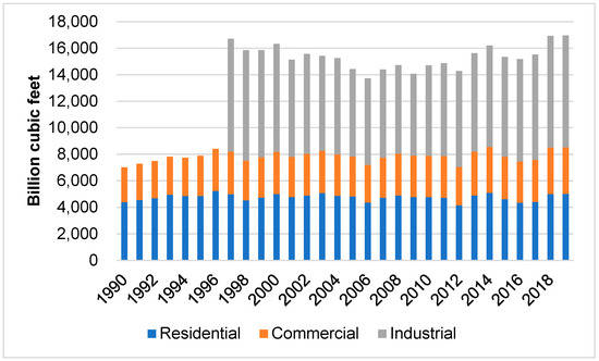
Figure 1. US annual natural gas consumption by end-use customer class in 1991–2019, recognizing that annual industrial consumption data are unavailable for years prior to 1997 (Data source: US Energy Information Agency).

Motivated by the preceding discussion, we estimate price responsiveness of residential demand for natural gas in the US. Informed by the thirteen selected studies reviewed below, our panel data analysis uses five parametric specifications: double-log, linear, constant elasticity of substitution (CES), Generalized Leontief (GL), and Transcendental logarithmic (TL) [7]. These models yield vastly different formulae for calculating residential natural gas demand’s own-price elasticity, which may be responsible for the diverse elasticity estimates reported in Table 1 and Table A1. (As our intent is to investigate how these specifications affect the own-price elasticity’s calculation, we do not perform statistical tests for determining which specification can yield empirical findings that best comply with the theoretical properties of an energy cost function [8]).

Table 1. Selected surveys on own-price elasticity estimates of residential natural gas demand.

Study	Short Run	Long Run
Gillingham et al. (2009) [9]	−0.14 to −0.44	−0.32 to −1.89
Al-Sahlawi (1989) [10]	−0.05 to −0.68	−1.06 to −3.42
Bohi and Zimmerman (1984) [11]	−0.05 to −0.60	−0.26 to −3.17

Our paper is academically interesting and policy important because accurate price elasticity estimates are necessary for energy policy modelling [12,13], resource planning [14,15,16,17], and demand projection [18,19,20]. They are also useful in analyzing the demand reduction effects due to carbon taxes [21], the size of price-induced demand reduction [22], an energy system’s responses to price shocks [23], optimal pricing [24], and welfare assessment of market liberalization [25]. Further, natural gas shortage adversely affects an economy [26,27]. As will be shown below, high price responsiveness implies low natural gas shortage cost. Hence, accurate price elasticity estimates aid efficient management of a natural gas shortage (e.g., New England’s shortage due to insufficient capacity to serve the region’s winter peak demand) (For an account of New England’s winter natural gas shortage, see [28]. Recent information on New England’s natural gas woes is available at https://www.cmu.edu/tepper/news/stories/2021/june/new-england-natural-gas-constraints.html (accessed on 22 April 2022)).

To provide our paper’s contextual background, we review 13 selected studies of the US residential natural gas demand (Unintended to be exhaustive, the selected studies are found via a two-step process: (1) use scholar.google.com to find an initial list with the keywords “price elasticity”, “residential natural gas demand” and “United States”; and (2) shorten the list by considering each study’s relevance to this analysis). Our literature review is intentionally brief, thanks to antecedent surveys of natural gas demand [10] and energy demands [11,29,30,31,32,33,34,35].

Table A1 summarizes own-price elasticity estimates from various studies, yielding the following remarks. First, these studies have geographic coverage from a single state to the entire nation. Second, ten studies use annual data, with the remainder using monthly data to better model the impacts of prices and weather on residential natural gas consumption. Third, inter-fuel substitution by residential customers is captured by fuel oil and electricity prices as additional regressors in 12 studies (While a residential customer may use natural gas as the primary fuel for cooking, space heating and water heating, inter-fuel substitution can still occur. Good examples include natural gas oven vs. microwave oven, central gas space heater vs. portable electric room heater, and central gas water heater vs. electric kettle). Fourth, the double-log specification is the most popular and used in 11 studies. The remaining two studies use linear and GL specifications. None use the CES and TL specifications, despite their popularity in energy demand analyses as noted by [7]. Fifth, a wide range of econometric estimation methods are used. Sixth, all studies rely upon average price data. Finally, the elasticity estimates in the last three columns indicate highly diverse price responsiveness.

Our literature review suggests the following knowledge gaps (KG):

• KG1: None of the studies considers how price responsiveness has changed over time.
• KG2: None of the studies investigates how price responsiveness differs by season.
• KG3: Little is known about how the parametric specification employed in the study may yield different results. While the critical issue of parametric specification is decades old [36], all 13 studies presume a particular specification (e.g., the double-log or GL) sans consideration of known alternatives like the linear, CES, and TL.
• KG4: None of the studies estimates the impact of cross-section dependence (CD) on the resulting price elasticity estimates.
• KG5: Regional variations in the responsiveness of natural gas to price changes has not been updated recently, as the study by [37] is already 35 years old.
• KG6: None of the studies uses own-price elasticity estimates to quantify natural gas shortage costs, thus overlooking demand response (DR) programs for efficient shortage management.

Our paper has salient features not found in the extant US studies listed in Table A1. First, it uses a large and recent sample of 17,280 monthly observations (=48 states × 30 years × 12 months per year) for estimating the US residential natural gas demand’s static, short-run and long-run own-price elasticities. Second, it documents the highly significant presence of CD possibly caused by common shocks due to factors such as federal government policies and regional weather patterns, and interdependence of regression error terms among states [38]. Third, it reports that erroneously ignoring CD presence tends to shrink the size of own-price elasticity estimates. Fourth, its monthly own-price elasticity estimates help determine seasonality in price responsiveness. Fifth, its regional own-price elasticity estimates update those found 35 years ago. Sixth, its rolling-window approach documents the nonlinear time trend of the US residential natural gas demand’s modest price responsiveness. This lends support to the continuation of energy efficiency standards, and demand-side-management programs as price-induced conservation via carbon taxes and other means may alone be insufficient to induce deep decarbonization [4,5]. Seventh, it applies own-price elasticity estimates to calculate natural gas shortage costs, underscoring the usefulness of residential demand response programs enabled by smart metering for efficient management of natural gas shortage.

Our paper’s newly found empirics provide useful input to energy modelers, demand forecasters and energy policy makers. They represent six contributions to the literature of residential natural gas demand:

(1)

The US residential demand for natural gas is price inelastic, with statistically significant (p-value ≤ 0.05) estimates of −0.271 to −0.486 for the static own price elasticity, −0.238 to −0.555 for the short run own price elasticity, and −0.323 to −0.796 for the long-run own price elasticity, matching the mid-range estimates of the studies listed in Table A1.

(2)

Parametric specification, CD presence, and partial adjustment have statistically significant effects on the own-price elasticity estimates of the US residential natural gas demand.

(3)

Erroneously ignoring the highly significant presence of CD tends to shrink the size of the own-price elasticity estimates of the US residential natural gas demand.

(4)

The US residential natural gas demand’s own-price elasticity estimates vary seasonally and regionally.

(5)

The US residential natural gas demand’s price responsiveness exhibits a nonlinear time trend.

(6)

A hypothetical one-day natural gas shortage that triggers curtailment of 10% of residential demand increases residential energy cost by less than 1%.

The rest of our paper proceeds as follows. Section 2 discusses nonlinear pricing of residential natural gas consumption and our empirical methodology. Section 3 presents our empirical findings. Section 4 contains conclusions, policy implications, and caveats.

2. Materials and Methods

2.1. Nonlinear Pricing of Residential Natural Gas Consumption

A residential customer typically faces a two-part tariff with a fixed customer charge ($/customer-month) and a volumetric charge ($/Mcf) that may follow an inclining block design [39]. If the volumetric charge is linear, the monthly average price (which is obtained by dividing the monthly bill by monthly usage) declines as usage increases because of the fixed customer charge. When the volumetric charge has an inclining block structure, the observed relationship between average price data and usage data is positive, even if the customer has a downward sloping demand curve.

The EIA’s monthly average price data are used in our panel data analysis because absent disaggregate consumption data and tariff information at customer level, accurate marginal prices such as those used by [39] are impossible to obtain. Further, should the average price data be found to cause estimation bias, instrumental variables (IV) estimation could be used to obtain the demand curve’s consistent coefficient estimates [40].

2.2. Five Parametric Specifications

Residential natural gas demand is a derived input determined from a household’s two-stage cost minimization in connection to the theory of home production [41,42]. Conditional on an installed stock of energy using durables in Stage 1, the household consumes natural gas Y₁ (Mcf) at price P₁ ($/Mcf), along with fuel oil Y₂ (gallon) at P₂ ($/gallon) (We do not consider propane for two reasons. First, none of the studies uses propane price as a regressor. Second, residential propane consumption is relatively minor in the US), and electricity Y₃ (kWh) at price P₃ ($/kWh) to minimize its monthly energy cost for producing an intermediate output Z = increasing function of end-use requirements for space heating, water heating, cooking, etc.:

C = P₁ Y₁ + P₂ Y₂ + P₃ Y₃.

(1)

The resulting natural gas demand is determined by energy price ratios as opposed to the levels of prices, based on the theory of cost duality [42,43] (As part of our final checks, we document that using price level data fails to materially change the double-log specification‘s own-price elasticity estimates). In Stage 2, the household selects an optimal mix of Z to maximize its utility while satisfying the monthly budget constraint.

For clarity and completeness, we reproduce the five specifications recently used to analyze the US industrial natural gas demand [7]. Should the estimated elasticities by specification be numerically close, they would be deemed robust for applications listed in Section 1.

The double-log demand equation is:

lnY₁ = β₀ + β₁ ln(P₁/P₃) + β₂ ln(P₂/P₃) + β_Z lnZ.

(2)

The own-price elasticity, ε = β₁, does not vary by consumption level or across time and states. Since the data for Z are unobservable, we assume that lnZ is a linear function of employment X, cooling degree days CDD and heating degree days HDD. This assumption makes sense because rising employment implies less time at home but higher income in turn affects end-use requirements. Further, space and water heating requirements are lower in warm weather than cold weather.

The linear demand equation is:

Y₁ = α₀ + α₁ (P₁/P₃) + α₂ (P₂/P₃) + α_Z Z.

(3)

It is assumed that the unobservable Z is a linear function of the variables X, CDD, and HDD. The own price elasticity is:

ε = α₁ (P₁/P₃)/Y₁.

(4)

As ε nonlinearly depends on (P₁/P₃) and Y₁, it varies by consumption level, price ratios, and across states and time. Thus, the estimated ε value for the entire US is the arithmetic mean of state- and month-specific estimates of the panel.

Under the CES specification, the natural gas—electricity consumption ratio equation is:

ln(Y₁/Y₃) = φ₀ + φ₁ ln(P₁/P₃),

(5)

We assume that φ₀ is a linear function of the variables X, CDD, and HDD to account for possible dependence of ln(Y_1/Y₃) on non-price factors. The own-price elasticity is:

ε = φ₁ (1 − S),

(6)

where S = P₁ Y₁/C is the cost share for natural gas ([3]). Since ε varies across states and time, the overall national value is the arithmetic mean of the state- and month-specific estimates of the panel.

When calculating ε based on Equation (6), we encounter a data mismatch problem. Specifically, Equation (6) requires state-level monthly data for residential fuel oil prices and consumption. However, the EIA does not publish data by customer class at monthly periodicity. We follow the procedures detailed in [7] to overcome this data mismatch.

The GL demand equation is:

Y₁ = b₁₁ + b₁₂ (P₂/P₁)^1/2 + b₁₃ (P₃/P₁)^1/2 + b_1Z Z.

(7)

Estimating Equation (7) assumes that Z is a simple linear function of the variables X, CDD, and HDD. The own-price elasticity is calculated as:

ε = −1/2 [b₁₂ (P₂/P₁)^1/2 + b₁₃ (P₃/P₁)^1/2]/Y₁.

(8)

As ε varies by the level of consumption, price ratios, and across states and time, its estimated value for the US is the arithmetic mean of state- and month-specific estimates of the panel.

The natural gas cost share equation used to estimate the TL model is:

S = a₁ + a₁₁ ln(P₁/P₃) + a₁₂ ln(P₂/P₃) + a_1Z lnZ,

(9)

where S = P₁ Y₁/C = natural gas cost share. Equation (9) assumes that lnZ is a simple linear function of the variables X, CDD, and HDD. The own-price elasticity is:

ε = (a₁₁ + S² − S)/S.

(10)

The estimated value for the nation is again the arithmetic mean of state- and month-specific estimates of the panel.

2.3. Long-Run Elasticity

A household’s current consumption likely depends on past consumption since a household’s stock of equipment using natural gas may change slowly over time. Hence, we include a lagged dependent variable as additional regressor to characterize the partial adjustment process, as similarly done by some studies in Table A1.

Let φ denote the lagged dependent variable’s coefficient. As will be seen in Section 3 below, the estimate for φ is between 0.263 and 0.344 (p-values ≤ 0.05). After using the own-price elasticity formula to compute the short-run elasticity (ε-sr) for each of the five parametric specifications that we use in this paper, we calculate the long-run elasticity (ε-lr) as follows: ε-lr = ε-sr/(1−φ).

2.4. Estimation of Residential Shortage Cost

Consider a hypothetical natural gas shortage with advance notice that enables a household to adjust its domestic activities. The natural gas shortage cost may be estimated as a percentage increase in residential energy cost using the following steps:

(1)

Consider a one-day shortage of natural gas that triggers curtailment of D% of the residential customer class’s total demand. The size of D is the same for all customer classes if the shortage triggers proportional rationing. However, D may vary by customer class, depending on the established curtailment protocol. For safety and health reasons, the protocol may curtail residential demand relatively less than non-residential demand.

(2)

Find the virtual price VP₁ ≡ (1 + ΔlnP₁) that renders D unnecessary, where ΔlnP₁ = −(D/ε) [44].

(3)

Estimate the cost of a one-day shortage of natural gas as a percentage of C:

SC = (ΔC/C) ÷ 30 days,

(11)

where ΔC = [∂C/∂P₁] ΔP₁ = Y₁ ΔP₁ using Shephard’s Lemma [45]. Since (ΔP₁/P₁) = ΔlnP₁, we find:

SC = (P₁ Y₁/C) (ΔP₁/P₁) ÷ 30 days = −S (D/ε) ÷ 30 days.

(12)

As an example, S = 20%, D = 10%, and ε = −0.1 implies SC = 20% ÷ 30 days per month = 0.67% of monthly energy cost.

The SC estimates based on Equation (12) assume that households do not incur such costs as lost production, idle labor, and material damage that are more related to non-residential customers [46]. This assumption makes sense because (a) the natural gas shortage implies partial curtailment rather than complete interruption of natural gas service; and (b) residential end-use requirements of space heating, water heating, and cooking can be partially met by electricity using durables (e.g., portable electric heater, electric kettle, and microwave oven).

To illustrate the dependence of SC on parametric specification and elasticity type, we use the 2019 cost share of natural gas and the three types of own-price elasticity estimates by specification. As SC increases with the cost share of natural gas (S), the extent of shortage (D), and the size of ε, a particular specification that yields relatively large elasticity estimates will lead to relatively small SC estimates.

2.5. Data Description

Descriptive statistics for our panel data are presented in Table 2. All variables have wide ranges in their values. The weather variables are more volatile than the other variables according to the coefficient of variation (=standard deviation/mean). The last column of Table 2 reports the pairwise correlations between Y₁ and the other variables. Y₁ is negatively correlated with P₁ (r = −0.247) as well as the price ratio (P₁/P₃) (r = −0.144) but uncorrelated with (P₂/P₃) (r = 0.002). Y₁ is also positively correlated with X (r = 0.115) and HDD (r = 0.824) but not with CDD (r = −0.458). These correlation coefficients are largely consistent with our expectations, though they fail to measure the marginal impacts of price ratios, employment, and weather on the US residential natural gas demand. Thus, we undertake the estimation strategy described below.

Table 2. Descriptive statistics for monthly data from Jan-1990 to Dec-2019 for the lower 48 states; number of observations = 17,280.

Variable (Source)	Definition	Mean	Standard Deviation	Minimum	Maximum	Correlation with Y1
Y1 (EIA and BLS)	Per capita consumption of natural gas (Mcf)	1.77	1.69	0.02	11.61	1.0
Y3 (EIA and BLS)	Per capita consumption of electricity (kWh)	618.40	956.64	21.47	11,598.17	−0.044
P1 (EIA)	Natural gas price ($/Mcf)	11.10	4.89	2.42	41.56	−0.247
P2 (EIA)	Fuel oil price ($/gallon)	1.56	0.96	0.34	4.34	−0.057
P3 (EIA)	Electricity price ($/kWh)	0.010	0.003	0.00	0.02	−0.122
P1/P3	Natural gas—electricity price ratio	1138.66	431.51	364.46	4664.42	−0.144
P2/P3	Fuel oil—electricity price ratio	154.44	84.37	27.57	574.36	0.002
X (BLS)	Per capita industrial employment	0.59	0.05	0.43	0.83	0.115
CDD (NOAA)	Cooling degree days	91.01	144.01	0	761	−0.458
HDD (NOAA)	Heating degree days	435.19	422.63	0	2111	0.824

Notes: (1) Data sources are from the US Energy Information Administration (EIA), the US Bureau of Labor Statistics (BLS), and the US National Oceanic and Atmospheric Administration (NOAA). (2) This table excludes the fuel oil consumption by the residential customer class due to the absence of monthly data from the EIA.

2.6. Estimation Strategy

As our data and regressions are susceptible to cross-section dependence, we adopt the dynamic common correlated effects (DCCE) panel estimator [47] to estimate the demand equations. The DCCE estimator includes current and lagged cross-section averages of all variables in the model as extra regressors. The DCCE estimator is consistent when the estimation includes enough lags of cross-section averages. Illustrating with the double-log model with partial adjustment, the estimable equation is:

$$\begin{gathered} \ln Y_{1it}={\eta }_i+{\beta }_1\ln (P_{1it}/P_{3it})+{\beta }_2\ln (P_{2it}/P_{3it})+{\beta }_3{X}_{it}+{\beta }_4{CDD}_{it}+{\beta }_5{HDD}_{it} \\ +\phi \ln Y_{1it-1}+{{\displaystyle \sum }}_{m=0}^M{\theta }_{1m}\ln \overline{(\frac{P_{1it-m}}{P_{3it-m}})}+{{\displaystyle \sum }}_{m=0}^M{\theta }_{2m}\ln \overline{(\frac{P_{2it-m}}{P_{3it-m}})}+{{\displaystyle \sum }}_{m=0}^M{\theta }_{3m}{\overline{X}}_{it-m} \\ +{{\displaystyle \sum }}_{m=0}^M{\theta }_{4m}{\overline{CDD}}_{it-m}+{{\displaystyle \sum }}_{m=0}^M{\theta }_{5m}{\overline{HDD}}_{it-m}+{{\displaystyle \sum }}_{m=0}^M{\theta }_{6m}{\overline{Y}}_{1it-1-m}+{\mu }_{it}, \end{gathered}$$

(13)

where η_i represents the state-specific fixed effect, μ_it represents the random error, i = 1 to 48 denotes the state, t = 2 to 360 denotes the time period and cross-section averages are indicated by a bar on top of the variable. When the estimate of φ is positive and statistically significant, short- and long-run elasticities may be estimated using the formulas presented in Section 2.3.

Equation (13) encompasses several panel data models as special cases. We impose the restriction of φ = 0 to obtain the static elasticity estimates. As only current cross-section averages are required in this case (M = 0), the equation will be estimated with the more parsimonious [48] common correlated effects estimator. For comparison, we also estimate the demand models without accounting for cross-section dependence (i.e., CD absence). In such cases, all θ coefficients are restricted to zero and the models will be estimated by the [49] mean group estimator.

Stated below is our multistep estimation strategy:

(1)

Test for CD in the variables using the test developed by [50].

(2)

Determine whether the variables are non-stationarity using the [51] panel unit root test that accounts for CD.

(3)

For each parametric specification, estimate the coefficients of Equation (13) with IV and non-IV estimation for the four cases formed by (a) φ = 0 vs. φ > 0; and (b) CD presence vs. CD absence. The instruments for the current month’s price-ratio are the lagged price ratios in the prior three months (The lagged price ratios in month t are pre-determined variables as they use average prices based on billing data in the prior three months. As the lagged price ratios are suitable instruments as they are highly correlated with the current price ratio (r ≥ 0.8)).

(4)

For each parametric specification, use the Durbin-Wu-Hausman test [52] to determine if current price ratios are endogenous and whether IV estimation is necessary.

3. Results

3.1. Tests of Cross-Section Independence and Non-Stationary Variables

Table 3 provides the results of tests which decisively reject (p-value < 0.01) the null hypotheses of cross-section independence and variable non-stationarity. Hence, our panel data analysis accounts for CD presence and without a concern regarding spurious regressions [53].

Table 3. Test statistics for cross-section independence and non-stationarity; p-values in ( ).

Variable	H0: Cross-Section Independence	H0: Non-Stationarity
Y1	584.87 (0.000)	−6.120 (0.000)
P1/P3	459.84 (0.000)	−5.132 (0.000)
P2/P3	614.44 (0.000)	−4.643 (0.000)
X	401.97 (0.000)	−3.403 (0.000)
CDD	569.56 (0.000)	−6.190 (0.000)
HDD	605.90 (0.000)	−6.190 (0.000)

3.2. General Observations

The regression results provided in Table 4 support three general observations. First, with one exception, all specifications have adjusted R² values ≥ 0.95 that indicate remarkable goodness of fit. Second, the hypothesis of cross-section independence is decisively rejected (p-value < 0.01) for each of the specifications. Third, our application of the Durbin-Wu-Hausman test suggests that the current price ratio data do not cause estimation bias under the empirically valid assumption of CD presence. These observations lead to our preferred regression results by specification, which are shaded in light green in the panels of Table 4. All preferred regressions are based on CD presence and non-IV estimation.

Table 4. Regression results by specification; coefficient and elasticity estimates which are statistically significant (p-value ≤ 0.10) are in bold; coefficient and elasticity estimates with an unexpected sign are in italic; and each specification’s preferred results shaded in light green.

Variable		CD Presence		CD Absence
		IV Estimation: No	IV Estimation: Yes	IV Estimation: No	IV Estimation: Yes
Panel A.1: Double-log specification without partial adjustment
RMSE		0.12	0.12	0.23	0.23
Adjusted R2		0.98	0.99	0.92	0.92
ln(P1/P3) = ln(natural gas price/electricity price)		−0.396	−0.334	−0.326	−0.507
ln(P2/P3) = ln(fuel oil price/electricity price)		0.309	0.262	−0.013	0.046
X = per capita employment		−0.419	−0.326	1.203	2.068
CDD = cooling degree days		0.000	0.000	−0.001	−0.001
HDD = heating degree days		0.001	0.001	0.002	0.002
Static own-price elasticity		−0.396	−0.334	−0.326	−0.507
p-value for testing H0: CD is absent		−	−	0.000	0.000
p-value for testing H0: natural gas price ratio data are exogeneous		0.995		0.017
Panel A.2: Double-log specification with partial adjustment
RMSE		0.09	0.09	0.15	0.15
Adjusted R2		0.99	0.99	0.97	0.97
ln(P1/P3) = ln(natural gas price/electricity price)		−0.336	−0.013	−0.167	0.019
ln(P2/P3) = ln(fuel oil price/electricity price)		0.186	0.029	−0.017	−0.076
X = per capita employment		0.171	0.045	1.446	0.641
CDD = cooling degree days		0.000	0.000	−0.001	−0.001
HDD = heating degree days		0.001	0.001	0.002	0.002
Lagged lnY1		0.271	0.296	0.308	0.316
Short-run own-price elasticity		−0.336	−0.013	−0.167	0.019
Long-run own-price elasticity		−0.460	−0.018	−0.242	0.028
p-value for testing H0: CD is absent		−	−	0.000	0.000
p-value for testing H0: natural gas price ratio data are exogeneous		0.352		0.000
Panel B.1: Linear specification without partial adjustment
RMSE		0.00	0.00	0.00	0.00
Adjusted R2		0.98	0.98	0.93	0.93
(P1/P3) = (natural gas price/electricity price)		−0.0002	−0.0003	0.0000	−0.0003
(P2/P3) = (fuel oil price/electricity price)		0.0013	0.0017	−0.0011	−0.0005
X = per capita employment		0.0000	0.0001	−0.0016	−0.0001
CDD = cooling degree days		0.0000	0.0000	0.0000	0.0000
HDD = heating degree days		0.0000	0.0000	0.0000	0.0000
Static own-price elasticity		−0.486	−0.684	0.018	−0.651
p-value for testing H0: CD is absent		−	−	0.000	0.000
p-value for testing H0: natural gas price ratio data are exogeneous		0.617		0.042
Panel B.2: Linear specification with partial adjustment
RMSE		0.00	0.00	0.00	0.00
Adjusted R2		0.99	0.99	0.97	0.97
(P1/P3) = (natural gas price/electricity price)		−0.0002	−0.0001	0.0001	0.0001
(P2/P3) = (fuel oil price/electricity price)		0.0012	0.0009	−0.0009	−0.0010
X = per capita employment		−0.0002	−0.0004	0.0001	0.0000
CDD = cooling degree days		0.0000	0.0000	0.0000	0.0000
HDD = heating degree days		0.0000	0.0000	0.0000	0.0000
Lagged Y1		0.303	0.304	0.299	0.301
Short-run own-price elasticity		−0.555	−0.337	0.177	0.262
Long-run own-price elasticity		−0.796	−0.485	0.253	0.375
p-value for testing H0: CD is absent		−	−	0.000	0.000
p-value for testing H0: natural gas price ratio data are exogeneous		0.437		0.591
Panel C.1: CES specification without partial adjustment
RMSE		0.13	0.13	0.26	0.26
Adjusted R2		0.98	0.98	0.91	0.91
ln(P1/P3) = ln(natural gas price/electricity price)		−0.354	−0.277	−0.518	−0.627
X = per capita employment		−0.765	−0.756	1.182	1.564
CDD = cooling degree days		−0.001	−0.001	−0.003	−0.003
HDD = heating degree days		0.001	0.001	0.001	0.001
Static own-price elasticity		−0.271	−0.212	−0.396	−0.480
p-value for testing H0: CD is absent		−	−	0.000	0.000
p-value for testing H0: natural gas price ratio data are exogeneous		0.672		0.186
Panel C.2: CES specification with partial adjustment
RMSE		0.10	0.10	0.18	0.18
Adjusted R2		0.99	0.99	0.96	0.96
ln(P1/P3) = ln(natural gas price/electricity price)		−0.311	−0.016	−0.284	−0.132
X = per capita employment		0.014	−0.218	1.135	0.713
CDD = cooling degree days		−0.001	−0.001	−0.003	−0.003
HDD = heating degree days		0.001	0.001	0.001	0.001
Lagged lnY1		0.263	0.290	0.327	0.340
Short-run own-price elasticity		−0.238	−0.012	−0.217	−0.101
Long-run own-price elasticity		−0.323	−0.017	−0.323	−0.153
p-value for testing H0: CD is absent		−	−	0.000	0.000
p-value for testing H0: natural gas price ratio data are exogeneous		0.100		0.769
Panel D.1: GL specification without partial adjustment
RMSE		0.00	0.00	0.00	0.00
Adjusted R2		0.98	0.98	0.93	0.93
(P2/P1)1/2 = (fuel oil price/natural gas price) 1/2		0.0001	0.0002	0.0004	0.0008
(P3/P1)1/2 = (electricity price/natural gas price) 1/2		0.0010	0.0008	−0.0010	−0.0010
X = per capita employment		−0.0003	0.0004	−0.0015	−0.0005
CDD = cooling degree days		0.0000	0.0000	0.0000	0.0000
HDD = heating degree days		0.0000	0.0000	0.0000	0.0000
Static own-price elasticity		−0.453	−0.427	−0.041	−0.408
p-value for testing H0: CD is absent		−	−	0.000	0.000
p-value for testing H0: natural gas price ratio data are exogeneous		0.117		0.065
Panel D.2: GL specification with partial adjustment
RMSE		0.00	0.00	0.00	0.00
Adjusted R2		0.99	0.99	0.97	0.97
(P2/P1)1/2 = (fuel oil price/natural gas price) 1/2		0.0003	−0.0008	0.0001	0.0001
(P3/P1)1/2 = (electricity price/natural gas price) 1/2		0.0007	0.0029	−0.0008	−0.0008
X = per capita employment		−0.0001	−0.0012	0.0000	−0.0001
CDD = cooling degree days		0.0000	0.0000	0.0000	0.0000
HDD = heating degree days		0.0000	0.0000	0.0000	0.0000
Lagged Y1		0.305	0.297	0.295	0.297
Short-run own-price elasticity		−0.453	−0.237	0.138	0.206
Long-run own-price elasticity		−0.651	−0.336	0.197	0.293
p-value for testing H0: CD is absent		−	−	0.000	0.000
p-value for testing H0: natural gas price ratio data are exogeneous		0.763		0.234
Panel E.1: TL specification without partial adjustment
RMSE		0.02	0.02	0.04	0.04
Adjusted R2		0.97	0.98	0.87	0.87
ln(P1/P3) = ln(natural gas price/electricity price)		0.087	0.093	0.101	0.074
ln(P2/P3) = ln(fuel oil price/electricity price)		0.010	0.008	−0.021	−0.012
X = per capita employment		−0.134	−0.134	0.118	0.252
CDD = cooling degree days		−0.0001	−0.0001	−0.0003	−0.0003
HDD = heating degree days		0.0001	0.0001	0.0002	0.0002
Static own-price elasticity		0.377	0.459	0.562	0.207
p-value for testing H0: CD is absent		−	−	0.000	0.000
p-value for testing H0: natural gas price ratio data are exogeneous		0.684		0.393
Panel E.2: TL specification with partial adjustment
RMSE		0.02	0.02	0.03	0.03
Adjusted R2		0.98	0.98	0.95	0.95
ln(P1/P3) = ln(natural gas price/electricity price)		0.075	0.061	0.080	0.094
ln(P2/P3) = ln(fuel oil price/electricity price)		0.007	0.015	−0.016	−0.020
X = per capita employment		0.021	0.034	0.099	0.039
CDD = cooling degree days		−0.0001	−0.0001	−0.0002	−0.0002
HDD = heating degree days		0.0001	0.0001	0.0002	0.0002
Lagged lnY1		0.344	0.361	0.396	0.390
Short-run own-price elasticity		0.223	0.043	0.294	0.480
Long-run own-price elasticity		0.340	0.068	0.487	0.788
p-value for testing H0: CD is absent		−	−	0.000	0.000
p-value for testing H0: natural gas price ratio data are exogeneous		0.766		0.005
Panel F. Seasonal pattern of elasticity estimates based on CD presence and non-IV estimation
Specification j	Static Own−Price Elasticity Estimate	Short−Run Own−Price Elasticity Estimate		Long−Run Own−Price Elasticity Estimate
Results for all 12 months
(1) Double-log	−0.396	−0.336		−0.460
(2) Linear	−0.486	−0.555		−0.796
(3) CES	−0.271	−0.238		−0.323
(4) GL	−0.453	−0.453		−0.651
(5) TL	0.377	0.223		0.340
Results for the spring months of March, April and May
(1) Double-log	−0.396	−0.336		−0.460
(2) Linear	−0.292	−0.334		−0.478
(3) CES	−0.259	−0.227		−0.308
(4) GL	−0.328	−0.327		−0.470
(5) TL	0.005	−0.095		−0.144
Results for the summer months of June, July and August
(1) Double-log	−0.396	−0.336		−0.460
(2) Linear	−0.951	−1.086		−1.557
(3) CES	−0.314	−0.276		−0.374
(4) GL	−0.799	−0.799		−1.149
(5) TL	1.219	0.935		1.425
Results for the fall months of September, October and November
(1) Double-log	−0.396	−0.336		−0.460
(2) Linear	−0.577	−0.659		−0.945
(3) CES	−0.281	−0.247		−0.335
(4) GL	−0.532	−0.529		−0.761
(5) TL	0.413	0.250		0.381
Results for the winter months of December, January and February
(1) Double-log	−0.396	−0.336		−0.460
(2) Linear	−0.124	−0.141		−0.202
(3) CES	−0.229	−0.201		−0.272
(4) GL	−0.155	−0.155		−0.223
(5) TL	−0.127	−0.197		−0.301

3.3. Regression Details

Using our preferred regression results, the double-log specification (Panel A.1 of Table 4) shows that the US residential natural gas demand has a static own-price elasticity estimate of −0.396. Natural gas demand increases with HDD, while the marginal effects of employment and CDD are insignificant. Panel A.2 provides a short-run own-price elasticity estimate of −0.336. The short-run estimate is smaller in absolute value than the long-run estimate of −0.460 due to the coefficient estimate of 0.271 for lagged lnY₁.

Panels B.1 and B.2 show de minimis coefficient estimates for employment, CDD and HDD for the linear specification. The estimated static own-price elasticity of −0.486 is comparable to the estimate derived from the double-log specification. Short- and long-run estimates are −0.555 and −0.796, respectively, which are noticeably larger (in absolute values) than those obtained under the double-log specification.

Panel C.1 shows that ln(Y₁/Y₃) declines with ln(P₁/P₃) for the CES specification. The estimated coefficients on CDD and HDD suggest that weather has a small but statistically significant impact on the natural gas-electricity consumption ratio, while the estimated coefficient for employment is not statistically significant. The static own-price elasticity estimate is −0.271, and the short- and long-run estimates are −0.238 and −0.323. Hence, the CES specification generates estimates which are smaller than those based on the double-log and linear specifications.

Panel D.1 and D.2 show that the estimated coefficients for employment, CDD, and HDD are nearly zero under the GL specification. The static own-price elasticity estimate is −0.453, while the short- and long-run estimates are −0.453 and −0.651, in between those based on the linear and CES specifications.

For the TL specification, Panel E.1 and E.2 report anomalously positive own-price elasticity estimates. Consequently, we question the empirical appropriateness of the TL specification for characterizing the residential demand for natural gas in the US.

In summary, the own-price elasticity estimates in Table 4’s Panels A.1 to D.2 are moderately diverse, corroborating the mid-range estimates in Table A1.

3.4. Seasonal Pattern of Own-Price Elasticity Estimates

To explore KG2, Panel F of Table 4 presents seasonal own-price elasticity estimates for each model. The winter elasticity estimates are smaller in size than non-winter estimates, due chiefly to a household’s winter space heating requirement.

3.5. Factors Affecting the US Residential Demand’s Empirical Price Responsiveness

Motivated by KG3 and KG4, a simple OLS dummy variable regression is used to delineate factors which affect our estimates of the price responsiveness of residential natural gas demand in the US. The results in Table 5 lead to the following inferences. First, the statistically insignificant coefficient estimates for F_j for j = 1 to 3 indicate that the double-log specification’s elasticity estimates resemble those of the linear, CES, and GL specifications. The large and significant estimate for F₄ reflects TL specification’s potential of yielding oddly positive price elasticity estimates. While the use of IV estimation does not seem to matter, ignoring CD presence can lead to smaller elasticity estimates due to the bias that CD absence introduces to the regression [47].

Table 5. OLS dummy variable regression; the regressand is the own-price elasticity estimate for US residential natural gas demand; sample size = 60 observations = 5 specifications × 2 estimation methods × 3 elasticity types × 2 CD assumptions.

	Estimate	Standard Error	p−Value
Adjusted R2	0.571
RMSE	0.235
Intercept	−0.249	0.076	0.002
F1 = 1 if linear specification, 0 otherwise	−0.013	0.106	0.903
F2 = 1 if CES specification, 0 otherwise	0.001	0.080	0.992
F3 = 1 if GL specification, 0 otherwise	0.048	0.079	0.541
F4 = 1 if TL specification, 0 otherwise	0.590	0.083	0.000
IV = 1 if IV estimation, 0 otherwise	0.063	0.061	0.306
SR = 1 if short−run, 0 otherwise	0.181	0.070	0.012
LR = 1 if long−run, 0 otherwise	0.174	0.081	0.036
CD = 1 if CD present, 0 otherwise	−0.260	0.061	0.000

3.6. Time Trend of Own-Price Elasticity Estimates

A 10-year rolling-window approach is adopted to estimate own-price elasticity under the double-log specification with cross-section dependence and non-IV estimation to address KG1. The first rolling-window period is Jan-1990 to Dec-2009, while the last period is Jan-2010 to Dec-2019. Figure 2 depicts a non-linear trend in the own-price elasticity of residential natural gas demand in the US, as confirmed by the results of OLS regressions appearing in Table 6. Nonetheless, the static and short-run estimates are between −0.4 and −0.5 and the long-run estimates are between −0.5 and −0.6, revealing the price-inelastic nature of US residential natural gas demand.

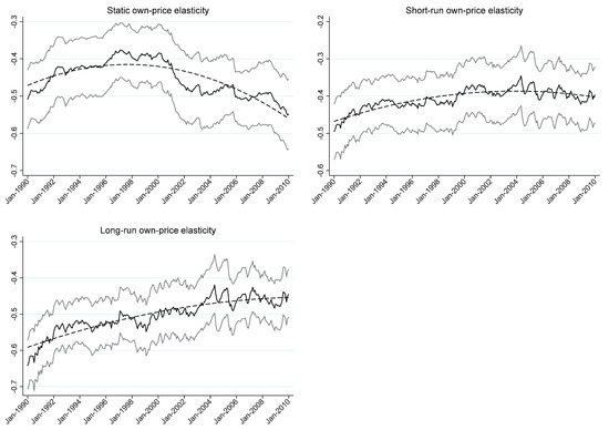
Figure 2. Rolling-window own-prices elasticity estimates. The solid black line portrays an elasticity estimate; the lower and upper solid grey lines show the 95% confidence interval; and the dashed line is the time trend of the estimate.

Table 6. OLS time trend regression: Own-price elasticity estimate = intercept + b₁ ID + b₂ ID² + error; sample size = 241 observations for each elasticity type.

Variable	Estimate	Standard Error	p−Value
Panel A: Static elasticity
Regressand’s mean	−0.452
Adjusted R2	0.715
RMSE	0.024
Intercept	−0.473	0.004	0.000
ID	0.0012	0.0001	0.000
ID2	−6.63 × 10−6	3.38 × 10−7	0.000
Panel B: Short−run elasticity
Regressand’s mean	−0.407
Adjusted R2	0.734
RMSE	0.014
Intercept	−0.469	0.003	0.000
ID	0.001	0.00005	0.000
ID2	−2.95 × 10−6	2.05 × 10−7	0.000
Panel C: Long−run elasticity
Regressand’s mean	−0.504
Adjusted R2	0.829
RMSE	0.019
Intercept	−0.593	0.005	0.000
ID	0.001	0.0001	0.000
ID2	−1.98 × 10−6	3.07 × 10−7	0.000

Note: The first observation (ID = 1) corresponds to the first 10-year period of 1990–1999, while the final observation (ID = 241) uses the last 10-year period of 2010–2019.

3.7. Residential Shortage Costs

Motivated by KG6, Table 7 reports shortage costs (SC) estimates for various parametric specifications and types of elasticities under the assumption of a one-day shortage that triggers curtailment of D = 10% of the residential demand for natural gas. We use the elasticity estimates from the preferred regressions shaded in light green in Table 4. For comparison, we also calculate SC using elasticity estimates from the regressions with CD absence and non-IV estimation. After dismissing the TL specification’s anomalous results, Panel A of Table 7 shows that residential shortage cost for a 10% demand curtailment is less than 1% of residential energy cost. Some of Panel B’s SC estimates are counter-intuitive, due chiefly to the empirically erroneous assumption of CD absence.

Table 7. Natural gas shortage cost for 2019 for various types of elasticities and specifications.

Parametric Specification	Static		Short−Run		Long−Run
	e1	SC	e1	SC	e1	SC
Panel A. CD presence and non−IV estimation
Double−log	−0.396	0.2%	−0.336	0.2%	−0.46	0.1%
Linear	−0.486	0.1%	−0.555	0.1%	−0.796	0.1%
CES	−0.271	0.2%	−0.238	0.3%	−0.323	0.2%
GL	−0.453	0.1%	−0.453	0.1%	−0.651	0.1%
TL	0.377	−0.2%	0.223	−0.3%	0.340	−0.2%
Panel B. CD absence and non−IV estimation
Double−log	−0.326	0.2%	−0.167	0.4%	−0.242	0.3%
Linear	0.018	−3.7%	0.177	−0.4%	0.253	−0.3%
CES	−0.396	0.2%	−0.217	0.3%	−0.323	0.2%
GL	−0.041	1.6%	0.138	−0.5%	0.197	−0.3%
TL	0.562	−0.1%	0.294	−0.2%	0.487	−0.1%

Notes: (1) The SC presented are the simple averages of all disaggregate SC numbers for each 2019 observation in the panel. (2) The SC estimates in Panel B are suspect because they erroneously ignore the highly significant CD presence.

3.8. Final Checks

We use the double-log specification with CD presence and non-IV estimation to perform several final checks on our analysis. Our choice of the double-log model reflects its popularity, as evidenced by Table A1 and empirical plausibility portrayed by Table 4.

We first repeat the panel data analysis after excluding the regressor representing the ratio of the price of fuel oil to the price of electricity. The static, short-run, and long-run elasticity estimates are −0.293, −0.281, and −0.390, respectively. Therefore, excluding fuel oil does not affect the own-price elasticity estimates in a material manner.

The second check uses aggregate, rather than per capita, energy usage and employment data when estimating the double-log regression model. Using aggregate data, we obtain price elasticity estimates that resemble those reported in Panels A.1 and A.2 of Table 4.

The third check uses price level data instead of price ratio data. We obtain an estimate for static price elasticity of −0.432, an estimate for the short-run own-price elasticity of −0.383, and an estimate for the long-run own-price elasticity of −0.518. Thus, the use of price level data does not materially alter the size of price elasticity estimates.

Motivated by KG5, the last check investigates regional price responsiveness. Table 8 shows that the Midwest and Northeast regions in Figure 3 have smaller (in absolute value) own-price elasticity estimates than the South and West regions. This makes sense because households residing in the Midwest and Northeast regions have higher space heating requirements caused by more severe winter weather than the South and West regions.

Table 8. Regional own-price elasticity estimates.

Region Definition	Static Elasticity	Short−Run Elasticity	Long−Run Elasticity
Midwest	−0.380	−0.317	−0.376
Northeast	−0.148	−0.166	−0.300
South	−0.439	−0.357	−0.492
West	−0.508	−0.400	−0.605

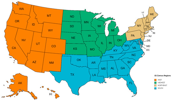
Figure 3. The four census regions in the US (map created by authors with mapchart.net).

4. Conclusions and Policy Implications

4.1. Conclusions

Our paper’s main conclusions are as follows. First, accurate price elasticity estimates are necessary for the important applications discussed in Section 1. Because of the highly diverse price elasticity estimates reported in extant surveys, such assumptions should come from a natural gas demand analysis of a large and recent sample of data. Second, employing monthly state-level data covering a long period is useful for estimating price responsiveness of residential natural gas demand. However, the analysis should recognize the effects of sample period, parametric specification, use of partial adjustment, treatment of CD, time trend, and region on the price elasticity estimates. Third, the US residential natural gas demand is price inelastic, with own-price elasticity estimates that match the mid-range of estimates reported by extant studies. Finally, the shortage cost estimates are less than 1% of residential energy cost for a 10% curtailment of residential natural gas demand.

4.2. Policy Implications

Our findings suggest that price-induced conservation’s projected demand-reduction is likely to be modest. Hence, achieving deep decarbonization may require strategies that do not rely on price induced changes on demand through carbon taxes and other means. Such a goal might require the continuation of energy efficiency standards and utility demand-side management programs.

Moreover, our empirics document that natural gas shortage costs vary by price responsiveness. As residential customers are heterogeneous (e.g., small homes with aging appliances vs. large homes with relatively new appliances) with diverse disaggregate price responsiveness [41,54], the US aggregate shortage cost could be reduced through demand response programs [55].

4.3. Limitations and Future Research

While the average price data used by this paper are in line with the practice of many prior studies in the literature, they lack details for a more granular analysis of price responsiveness (e.g., [39]). Further, while the effects of different parametric specifications on price elasticity estimates are explored in this paper, future research may consider using statistical tests for selecting the most appropriate specification (e.g., [8]). Finally, alternative dynamic specifications of the demand equations such as the Autoregressive Distributed Lag modelling (e.g., [38]) can be used to further explore the price responsiveness of residential demand for natural gas demand in the US.

References

- British Petroleum. Statistical Review of World Energy. 2021. Available online: https://www.bp.com/en/global/corporate/energy-economics/statistical-review-of-world-energy.html (accessed on 22 April 2022).
- Gillingham, K.; Huang, P. Is abundant natural gas a bridge to a low-carbon future or a dead-end? Energy J. 2019, 40, 1–26. [Google Scholar] [CrossRef] [Green Version]
- Woo, C.K.; Shiu, A.; Liu, Y.; Luo, X.; Zarnikau, J. Consumption effects of an electricity decarbonization policy: Hong Kong. Energy 2018, 144, 887–902. [Google Scholar] [CrossRef]
- Mahone, A.; Subin, Z.; Orans, R.; Miller, M.; Regan, L.; Calviou, M.; Saenz, M.; Bacalao, N. On the path of decarbonization. IEEE Power Energy Mag. 2018, 16, 58–68. [Google Scholar] [CrossRef]
- Williams, J.H.; DeBenedictis, A.; Ghanadan, R.; Mahone, A.; Moore, J.; Morrow, W.R.; Price, S.; Torn, M.S. The Technology Path to Deep Greenhouse Gas Emissions Cuts by 2050: The Pivotal Role of Electricity. Science 2012, 335, 53–59. [Google Scholar] [CrossRef] [Green Version]
- Zarnikau, J.; Woo, C.; Zhu, S.; Tsai, C. Market price behavior of wholesale electricity products: Texas. Energy Policy 2018, 125, 418–428. [Google Scholar] [CrossRef]
- Li, R.; Woo, C.K.; Tishler, A.; Zarnikau, J. How price responsive is industrial natural gas demand in the US? Util. Policy 2022, 74, 101318. [Google Scholar] [CrossRef]
- Tishler, A.; Lipovesky, S. The flexible CES-GBC family of cost functions: Derivation and application. Rev. Econ. Stat. 1997, 79, 638–646. [Google Scholar] [CrossRef]
- Gillingham, K.; Newell, R.G.; Palmer, K. Energy efficiency economics and policy. Annu. Rev. Resour. Econ. 2009, 1, 597–620. [Google Scholar] [CrossRef]
- Al-Sahlawi, M.A. The demand for natural gas: A survey of price and income elasticities. Energy J. 1989, 10, 77–90. [Google Scholar] [CrossRef]
- Bohi, D.R.; Zimmerman, M.B. An Update on Econometric Studies of Energy Demand Behavior. Annu. Rev. Energy 1984, 9, 105–154. [Google Scholar] [CrossRef]
- Hausman, J.A. Project Independence Report: An Appraisal of U.S. Energy Needs up to 1985. Bell J. Econ. 1975, 6, 517–551. [Google Scholar] [CrossRef]
- Manne, A.S.; Richels, R.G.; Weyant, J.P. Feature article—Energy policy modeling: A survey. Oper. Res. 1979, 27, 1–36. [Google Scholar] [CrossRef] [Green Version]
- Abrell, J.; Weigt, H. Investments in a combined energy network model: Substitution between natural gas and electricity? Energy J. 2016, 37, 63–86. [Google Scholar] [CrossRef]
- Çalci, B.; Leibowicz, B.D.; Bard, J.F. North American Natural Gas Markets Under LNG Demand Growth and Infrastructure Restrictions. Energy J. 2022, 43, 1–24. [Google Scholar] [CrossRef]
- Holz, F.; Richter, P.M.; Egging, R. The Role of Natural Gas in a Low-Carbon Europe: Infrastructure and Supply Security. Energy J. 2016, 37, 33–59. [Google Scholar] [CrossRef]
- Logan, J.; Lopez, A.; Mai, T.; Davidson, C.; Bazilian, M.; Arent, D. Natural gas scenarios in the U.S. power sector. Energy Econ. 2013, 40, 183–195. [Google Scholar] [CrossRef]
- Bianco, V.; Scarpa, F.; Tagliafico, L.A. Scenario analysis of nonresidential natural gas consumption in Italy. Appl. Energy 2014, 113, 392–403. [Google Scholar] [CrossRef]
- Dilaver, Ö.; Dilaver, Z.; Hunt, L.C. What drives natural gas consumption in Europe? Analysis and projections. J. Nat. Gas Sci. Eng. 2014, 19, 125–136. [Google Scholar] [CrossRef]
- Huntington, H.G. Industrial natural gas consumption in the United States: An empirical model for evaluating future trends. Energy Econ. 2007, 29, 743–759. [Google Scholar] [CrossRef]
- Xiang, D.; Lawley, C. The impact of British Columbia’s carbon tax on residential natural gas consumption. Energy Econ. 2019, 80, 206–218. [Google Scholar] [CrossRef]
- Rowland, C.S.; Mjelde, J.W.; Dharmasena, S. Policy implications of considering pre-commitments in U.S. aggregate energy demand system. Energy Policy 2017, 102, 406–413. [Google Scholar] [CrossRef]
- Brown, M.; Siddiqui, S.; Avraam, C.; Bistline, J.; Decarolis, J.; Eshraghi, H.; Giarola, S.; Hansen, M.; Johnston, P.; Khanal, S.; et al. North American energy system responses to natural gas price shocks. Energy Policy 2020, 149, 112046. [Google Scholar] [CrossRef]
- Gong, C.; Tang, K.; Zhu, K.; Hailu, A. An optimal time-of-use pricing for urban gas: A study with a multi-agent evolutionary game-theoretic perspective. Appl. Energy 2015, 163, 283–294. [Google Scholar] [CrossRef]
- Lee, J.-D.; Kim, T.-Y. Ex-ante analysis of welfare change for a liberalization of the natural gas market. Energy Econ. 2004, 26, 447–461. [Google Scholar] [CrossRef]
- Alcaraza, C.; Villalvazo, S. The effect of natural gas shortages on the Mexican economy. Energy Econ. 2017, 66, 147–153. [Google Scholar] [CrossRef] [Green Version]
- Leahy, E.; Devitt, C.; Lyons, S.; Tol, R.S. The cost of natural gas shortages in Ireland. Energy Policy 2012, 46, 153–169. [Google Scholar] [CrossRef] [Green Version]
- Charles, R.K.M. Regional Estimates of the Price Elasticity of Demand for Natural Gas in the United States. Master’s Thesis, Massachusetts Institute of Technology, Cambridge, MA, USA, 2016. Available online: https://dspace.mit.edu/handle/1721.1/104830 (accessed on 22 April 2022).
- Dahl, C. A Survey of Energy Demand Elasticities in Support of the Development of the NEMS; Colorado School of Mines: Golden, CO, USA, 1993. [Google Scholar]
- Dahl, C.; Roman, C. Energy Demand Elasticities—Fact or Fiction: A Survey; Colorado School of Mines: Golden, CO, USA, 2004. [Google Scholar]
- Hartman, R.S. Frontiers in Energy Demand Modeling. Annu. Rev. Energy 1979, 4, 433–466. [Google Scholar] [CrossRef] [Green Version]
- Huntington, H.G.; Barrios, J.J.; Arora, V. Review of key international demand elasticities for major industrializing economies. Energy Policy 2019, 133, 110878. [Google Scholar] [CrossRef] [Green Version]
- Labandeira, X.; Labeaga, J.M.; López-Otero, X. A meta-analysis on the price elasticity of energy demand. Energy Policy 2017, 102, 549–568. [Google Scholar] [CrossRef] [Green Version]
- Suganthia, L.; Samuel, A.A. Energy models for demand forecasting—A review. Renew. Sustain. Energy Rev. 2012, 16, 1223–1240. [Google Scholar] [CrossRef]
- Taylor, L.D. The demand for energy: A survey of price and income elasticities. In International Studies of the Demand for Energy; Nordhaus, W., Ed.; North Holland: Amsterdam, The Netherlands, 1977. [Google Scholar]
- Baxter, R.E.; Rees, R. Analysis of the Industrial Demand for Electricity. Econ. J. 1968, 78, 277–298. [Google Scholar] [CrossRef]
- Lin, W.T.; Chen, Y.H.; Chatov, R. The demand for natural gas, electricity and heating oil in the United States. Resour. Energy 1987, 9, 233–258. [Google Scholar] [CrossRef]
- Li, R.; Woo, C.K.; Cox, K. How price-responsive is residential retail electricity demand in the US? Energy 2021, 232, 120921. [Google Scholar] [CrossRef]
- Auffhammer, M.; Rubin, E. Natural Gas Price Elasticities and Optimal Cost Recovery under Consumer Heterogeneity: Evidence from 300 Million Natural Gas Bills. NBER Working Paper 24295. 2018. Available online: https://www.nber.org/papers/w24295 (accessed on 22 April 2022).
- Davidson, R.; Mackinnon, J.G. Estimation and Inference in Econometrics; Oxford University Press: Oxford, UK, 1993. [Google Scholar]
- Dubin, J.A.; Henson, S.E. An engineering/econometric analysis of seasonal energy demand and conservation in the Pacific Northwest. J. Bus. Econ. Stat. 1988, 6, 121–134. [Google Scholar]
- Woo, C.; Tishler, A.; Zarnikau, J.; Chen, Y. Average residential outage cost estimates for the lower 48 states in the US. Energy Econ. 2021, 98, 105270. [Google Scholar] [CrossRef]
- Diewert, W.E. An Application of the Shephard Duality Theorem: A Generalized Leontief Production Function. J. Political Econ. 1971, 79, 481–507. [Google Scholar] [CrossRef]
- Woo, C.K. Managing water supply shortage: Interruption vs. pricing. J. Public Econ. 1994, 54, 145–160. [Google Scholar] [CrossRef]
- Varian, H. Microeconomics Analysis; Norton: New York, NY, USA, 1992. [Google Scholar]
- Woo, C.; Tishler, A.; Zarnikau, J.; Chen, Y. A back of the envelope estimate of the average non-residential outage cost in the US. Electr. J. 2021, 34, 106930. [Google Scholar] [CrossRef]
- Chudik, A.; Pesaran, M.H. Common correlated effects estimation of heterogeneous dynamic panel data models with weakly exogenous regressors. J. Econ. 2015, 188, 393–420. [Google Scholar] [CrossRef] [Green Version]
- Pesaran, M.H. Estimation and inference in large heterogeneous panels with a multifactor error structure. Econometrica 2006, 74, 967–1012. [Google Scholar] [CrossRef] [Green Version]
- Pesaran, M.H.; Smith, R. Estimating long-run relationships from dynamic heterogeneous panels. J. Econom. 1995, 68, 79–113. [Google Scholar] [CrossRef]
- Pesaran, M.H. General diagnostic tests for cross-sectional dependence in panels. Empir. Econ. 2020, 60, 13–50. [Google Scholar] [CrossRef]
- Pesaran, M.H. A simple panel unit root test in the presence of cross-section dependence. J. Appl. Econom. 2007, 22, 265–312. [Google Scholar] [CrossRef] [Green Version]
- Wooldridge, J.M. Econometric Analysis of Cross Section and Panel Data; MIT Press: Cambridge, MA, USA, 2010. [Google Scholar]
- Baltagi, B.H.; Kao, C. Nonstationary panels, cointegration in panels and dynamic panels: A survey. In Nonstationary Panels, Panel Cointegration, and Dynamic Panels; Baltagi, B.H., Fomby, T.B., Carter Hill, R., Eds.; Advances in Econometrics; Emerald Group Publishing Limited: Bingley, UK, 2001; Volume 15, pp. 7–51. [Google Scholar]
- Lavín, F.V.; Dale, L.; Hanemann, M.; Moezzi, M. The impact of price on residential demand for electricity and natural gas. Clim. Chang. 2011, 109, 171–189. [Google Scholar] [CrossRef]
- Woo, C.; Sreedharan, P.; Hargreaves, J.; Kahrl, F.; Wang, J.; Horowitz, I. A review of electricity product differentiation. Appl. Energy 2014, 114, 262–272. [Google Scholar] [CrossRef]
- Beierlein, J.G.; Dunn, J.W.; McConnon, J.C. The demand for electricity and natural gas in the Northern United States. Rev. Econ. Stat. 1981, 63, 403–408. [Google Scholar] [CrossRef]
- Barnes, R.; Gillingham, R.; Hagemann, R. The short-run residential demand for natural gas. Energy J. 1982, 3, 59–72. [Google Scholar] [CrossRef]
- Blattenberger, G.R.; Taylor, L.D.; Rennhack, R. Natural Gas Availability and the Residential Demand for Energy. Energy J. 1983, 4, 23–45. [Google Scholar] [CrossRef]
- Liu, B.-C. Natural gas price elasticities: Variations by region and by sector in the USA. Energy Econ. 1983, 5, 195–201. [Google Scholar] [CrossRef]
- Garcia-Cerritti, L.M. Estimating elasticities of residential energy demand from panel county data using dynamic random variables models with heteroskedastic and correlated error terms. Resour. Energy Econ. 2000, 22, 355–366. [Google Scholar] [CrossRef]
- Bernstein, M.A.; Griffin, J. Regional Differences in the Price-Elasticity of Demand for Energy; Rand Corporation: Santa Monica, CA, USA, 2005. [Google Scholar]
- Payne, J.E.; Loomis, D.; Wilson, R. Residential natural gas demand in Illinois: Evidence from the ARDL bounds testing approach. J. Reg. Anal. Policy 2011, 41, 138–147. [Google Scholar]
- Gautam, T.K.; Paudel, K.P. The demand for natural gas in the Northeastern United States. Energy 2018, 158, 890–898. [Google Scholar] [CrossRef]
- Burns, K. An investigation into changes in the elasticity of U.S. residential natural gas consumption: A time-varying approach. Energy Econ. 2021, 99, 105253. [Google Scholar] [CrossRef]
- Bartels, R.; Fiebig, D.; Plumb, M.H. Gas or electricity, which is cheaper? An econometric approach with application to Australian expenditure data. Energy J. 1996, 17, 33–77. [Google Scholar] [CrossRef]
- Wadud, Z.; Dey, H.S.; Kabir, M.A.; Khan, S.I. Modeling and forecasting natural gas demand in Bangladesh. Energy Policy 2011, 39, 7372–7380. [Google Scholar] [CrossRef] [Green Version]
- Berndt, E.R.; Watkins, G.C. Demand for Natural Gas: Residential and Commercial Markets in Ontario and British Columbia. Can. J. Econ. 1977, 10, 97–111. [Google Scholar] [CrossRef]
- Hu, W.; Ho, M.S.; Cao, J. Energy consumption of urban households in China. China Econ. Rev. 2019, 58, 101343. [Google Scholar] [CrossRef]
- Li, L.; Luo, X.; Zhou, K.; Xu, T. Evaluation of increasing block pricing for households’ natural gas: A case study of Beijing, China. Energy 2018, 157, 162–172. [Google Scholar] [CrossRef]
- Zeng, S.; Chen, Z.-M.; Alsaedi, A.; Hayat, T. Price elasticity, block tariffs, and equity of natural gas demand in China: Investigation based on household-level survey data. J. Clean. Prod. 2018, 179, 441–449. [Google Scholar] [CrossRef]
- Zhang, Y.; Ji, Q.; Fan, Y. The price and income elasticity of China’s natural gas demand: A multi-sectoral perspective. Energy Policy 2018, 113, 332–341. [Google Scholar] [CrossRef]
- Ackah, I. Determinants of natural gas demand in Ghana. OPEC Energy Rev. 2014, 38, 272–295. [Google Scholar] [CrossRef] [Green Version]
- Kostakis, I.; Lolos, S.; Sardianou, E. Residential natural gas demand: Assessing the evidence from Greece using pseudo-panels, 2012–2019. Energy Econ. 2021, 99, 105301. [Google Scholar] [CrossRef]
- Ota, T.; Kakinaka, M.; Kotani, K. Demographic effects on residential electricity and city gas consumption in the aging society of Japan. Energy Policy 2018, 115, 503–513. [Google Scholar] [CrossRef] [Green Version]
- Lim, C. Estimating Residential and Industrial City Gas Demand Function in the Republic of Korea—A Kalman Filter Application. Sustainability 2019, 11, 1363. [Google Scholar] [CrossRef] [Green Version]
- Yoo, S.-H.; Lim, H.-J.; Kwak, S.-J. Estimating the residential demand function for natural gas in Seoul with correction for sample selection bias. Appl. Energy 2009, 86, 460–465. [Google Scholar] [CrossRef]
- Kahn, M.A. Modelling and forecasting the demand for natural gas in Pakistan. Renew. Sustain. Energy Rev. 2015, 49, 1145–1159. [Google Scholar] [CrossRef]
- Erdogdu, E. Natural gas demand in Turkey. Appl. Energy 2010, 87, 211–219. [Google Scholar] [CrossRef] [Green Version]
- Alberini, A.; Khymych, O.; Ščasný, M. Responsiveness to energy price changes when salience is high: Residential natural gas demand in Ukraine. Energy Policy 2020, 144, 111534. [Google Scholar] [CrossRef]
- Asche, F.; Nilsen, O.B.; Tveteras, R. Natural gas demand in the European household sector. Energy J. 2005, 29, 27–46. [Google Scholar] [CrossRef] [Green Version]
- Estrada, J.; Fugleberg, O. Price Elasticities of Natural Gas Demand in France and West Germany. Energy J. 1989, 10, 77–90. [Google Scholar] [CrossRef]
- Bernstein, R.; Madlener, R. Residential Natural Gas Demand Elasticities in OECD Countries: An ARDL Bounds Testing Approach. 2011. Available online: https://papers.ssrn.com/sol3/papers.cfm?abstract_id=2078036 (accessed on 22 April 2022).
- Burke, P.J.; Yang, H. The price and income elasticities of natural gas demand: International evidence. Energy Econ. 2016, 59, 466–474. [Google Scholar] [CrossRef] [Green Version]
Publisher’s Note: MDPI stays neutral with regard to jurisdictional claims in published maps and institutional affiliations. |
© 2022 by the authors. Licensee MDPI, Basel, Switzerland. This article is an open access article distributed under the terms and conditions of the Creative Commons Attribution (CC BY) license (https://creativecommons.org/licenses/by/4.0/).