Article

Observer-Based H Load Frequency Control for Networked Power Systems with Limited Communications and Probabilistic Cyber Attacks

School of Electrical and Automation, Nanjing Normal University, Nanjing 210046, China
*
Authors to whom correspondence should be addressed.
Energies 2022, 15(12), 4234; https://doi.org/10.3390/en15124234
Submission received: 19 April 2022 / Revised: 23 May 2022 / Accepted: 7 June 2022 / Published: 8 June 2022
(This article belongs to the Special Issue Advances and Optimization of Electric Energy System)

Abstract

:
This paper studies load frequency control (LFC) for networked power systems with limited communications and probabilistic cyber attacks. Some restrictions exist during the information transmission, which can impair behavior and lead to instability of power systems. Throughout this paper, we consider such power systems that involve multi-path missing measurements and input–output time-varying delays as well as cyber attacks in the communication channels. A feedback controller is presented, which is based on the observer to implement H LFC for power systems with disturbance rejection level γ . By Lyapunov stability theory, adequate criteria are given to ensure the stable operation of power systems. Finally, the validity of theoretical analysis is demonstrated and illustrated by numerical simulations.

Graphical Abstract

1. Introduction

Load frequency control (LFC) is a scheme that can control the output power of generators set so that instantaneous frequency deviation in each region and the power exchange between regions are kept within the specified range, and their steady-state error is equal to zero [1,2]. Traditional LFC schemes transmit measurement signals and control signals with the help of a purpose-built communication infrastructure [3,4]. LFC in modern power systems mainly applies open communication facilities to transmit the above-mentioned signals. On account of the inherent properties of open communication, time-varying delays and packet dropout, as well as cyber attacks, are inevitable, seriously affecting the efficiency of load frequency control schemes [5,6]. The issue of the LFC of power systems with delays as well as packet dropout and cyber attacks have received extensive attention in recent years [7,8,9,10,11].
In the last few years, a good deal of results have been reported with regard to LFC problems of power systems containing packet dropout as well as time delays [6,12,13,14,15]. A novel decentralized LFC control strategy based on switching control theory was researched by Yang et al. By means of transmission delays as a switching decision parameter, the LFC system as a range of subsystems was modeled, which provides a more accurate description of the impact of delays as well as packet dropout on the system [6]. Zhang et al. proposed a delay-dependent robust method for the analysis of PID-based LFC schemes that take into account time delays [12]; however, for the problem of LFC in power systems, many researchers have only studied packet dropout or time delays in the output communication channels, ignoring the controller-to-actuator link [16]. Furthermore, to our knowledge, few researchers have investigated the LFC problem in power systems with delays as well as packet loss both in the controller-to-actuator link and output communication channels.
Along with the large-scale application of open communication networks in power systems, the matter of power system security has also attracted widespread attention from scholars. Cyber attacks can cause serious power incidents, especially if there are cyber attacks during data transmission [17]. Cyber attacks can be divided into denial of service attacks as well as deception attacks, of which, deception attacks pose the greatest threat to power systems. Deception attacks are attacks in which an attacker modifies the integrity of packets transmitted between different parts of the network in order to obtain critical information. A great deal of work is being undertaken in relation to deception attacks. Finite-time constrained and adaptive event-triggered control problems for networked systems involved in deception attacks were studied by Sathishkumar et al. [18]. Tian et al. submitted a memory-based event-triggered H LFC for power systems that involve deception attacks [19]. Adaptive event-triggered control of neural networks affected by double deception attacks and time-varying delays were researched by Shen et al. [20].
In addition, in order to control the system more efficiently, scholars adopt state feedback control; however, state variables cannot be measured directly from the system, which makes the implementation of state feedback techniques more complex than output feedback. Most previous work made the assumption that all system states are accessible. Tapin et al. presented a full-state feedback controller design for LFC loops based on the pole positioning method [21]. A state estimation was presented by Vrdoljak et al., which is based on rapid measurement output sampling with full state feedback [22]. Instead, only a fraction of the system state can be obtained in practice. Motivated by this point, many scholars are paying attention to state feedback control that is based on an observer. A means of quasi-decentralized LFC scheme of power systems that is based on a function observer was proposed by Tyrone et al. [23]. To realize a global state feedback controller, a new distributed function observer was designed by Thanh et al. [24]. It is notable that the problem of observer-based LFC in power systems that involve limited communications and probabilistic deception attacks have not yet been researched—this is the motivation behind our article.
The aim of this paper is to design an observer-based H LFC scheme for power systems with limited communications and probabilistic cyber attacks. Networked power systems with input and output delays and packet dropout as well as cyber attacks are considered in this article. The main contributions of this paper are given as follows:
(1)
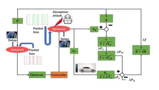
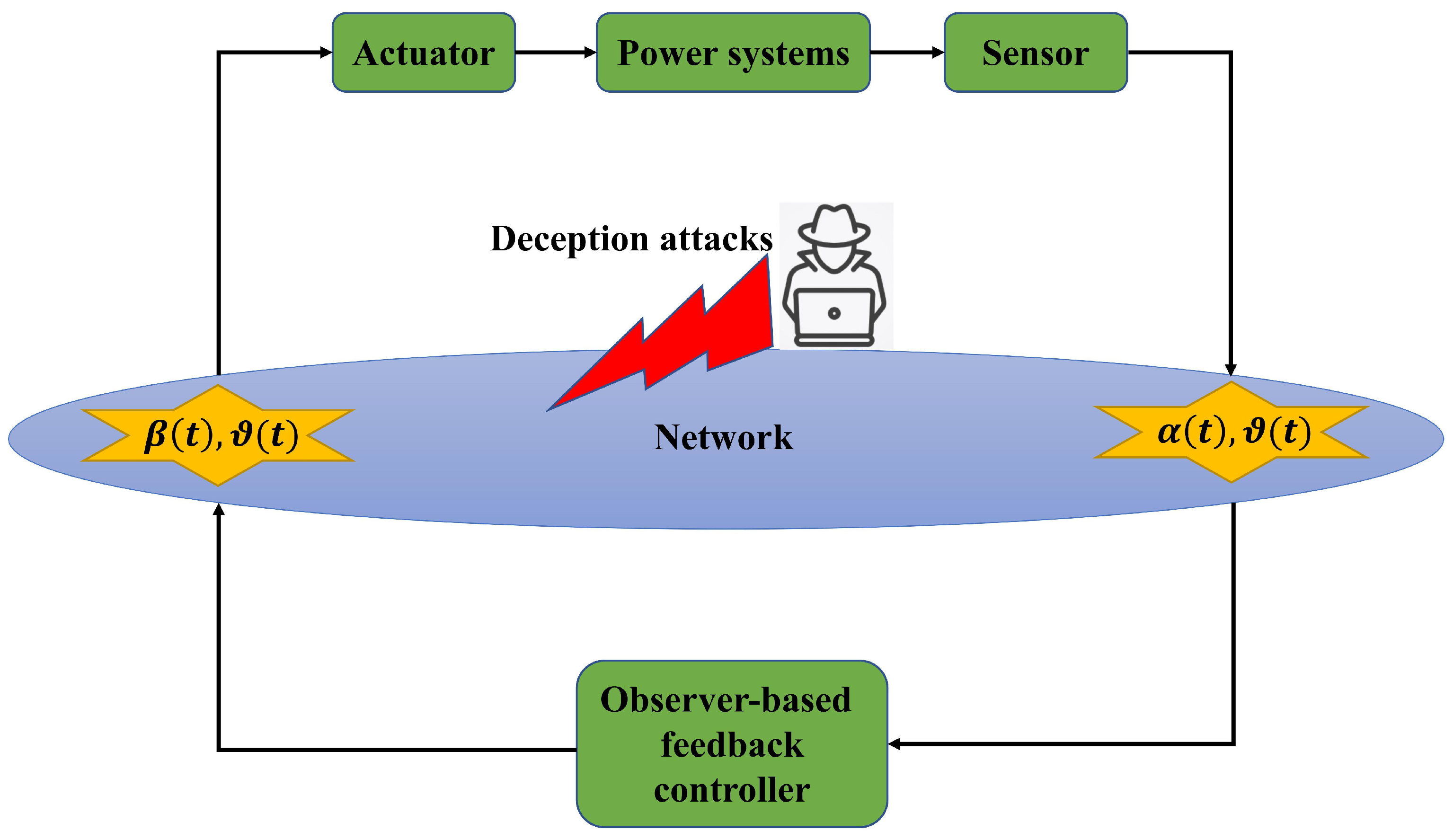
An observer-based LFC model is established for networked power systems, which not only takes into account multi-path missing measurements and input–output time-varying delays in the communication channel but also considers the influences of random cyber attacks on data transmission.
(2)
To implement the H load frequency controller, delay-dependent H stability criterion including time delays and packet dropout as well as cyber attacks phenomena are derived with the  help of Lyapunov–Krasovskii function approach in LMI framework.
(3)
On the basis of the resulting stability criteria, the stability gains of the observer and controller are calculated with the assistance of the LMI toolbox.
Notations: The transpose of the matrix L is represented by L T . X 1 represents its inverse matrix. The symmetric terms in the matrix are denoted by ∗. R n denotes the n-dimensional Euclidean space. R n × n is n × n real matrices. The diagonal matrix is denoted by d i a g { } . Identity matrix is denoted by I. · 2 denotes the usual 2 [ 0 , ) norm. E is the expectation operator. The probability when the stochastic variable x is equal to a is denoted by P r o b { x = a } . The dimension of these vectors and matrices will be cleared in the context.

2. Model Description and Preliminaries

In this paper, the structure of the power system’s LFC model is shown in Figure 1. The system model is represented as follows [25]:
x ˙ ( t ) = A x ( t ) + B u ( t ) + C w ( t ) , y ˜ ( t ) = D x ( t ) ,
where
x ( t ) = Δ f Δ P m Δ P v Δ P e T , ω ( t ) = P d , y ( t ) = A C E ( t ) , D = β 0 0 0 , B = 0 0 α g T g α e k e T e T , C = 1 M 0 0 0 , A = D M 1 M 0 1 M 0 1 T c h 1 T c h 0 1 T g R 0 1 T g 0 0 0 0 1 T e .
The parameters of the networked power systems, which are depicted in Figure 1, are listed in Table 1 [4,25].
As shown in Figure 2, considering the sudden changes in the operating environment as well as the jamming of the communication channels, the output communication channels are considered to be limited, that is, the output signal y ˜ ( t ) suffer from data missing α ( t ) and time-varying delays ϑ ( t ) ; therefore, the output signal will be described as
y ( t ) = α ( t ) y ˜ ( t ϑ ( t ) ) ,
time-varying delays that exist in the communication channels ϑ ( t ) satisfy
0 ϑ ( t ) ϑ M , ϑ ˙ ( t ) μ < ,
where ϑ M and μ are some given constants.
Remark 1.
That packet loss from the sensor to the controller in a networked control system (1) is expressed as  α ( t ) , which is a  Bernoulli stochastic variable. In particular, if the link fails, we have α ( t ) = 0 , otherwise α ( t ) = 1 if the data are successfully transmitted.
Moreover, we assume that
P r o f { α ( t ) = } = α , = 1 , 1 α , = 0 .
From the above analysis, we have the following networked power systems involving time-varying delays as well as missing output data measurements
x ˙ ( t ) = A x ( t ) + B u ( t ) + C w ( t ) , y ( t ) = α ( t ) ( D x ( t ϑ ( t ) ) ) .
We study the robustness of the networked power systems (4) by designing a feedback controller, which is based on an observer. Consider a controller with input missing measurements β ( t ) and time-varying delays ϑ ( t ) . Suppose that the deception attack restricted in Hypothesis 1 is performed as a nonlinear function f ( x ( t ϑ ( t ) ) ) .
x ^ ˙ ( t ) = A x ^ ( t ) + B u ( t ) + L [ y ( t ) α ( t ) D x ^ ( t ϑ ( t ) ) ] , u ( t ) = ( 1 θ ( t ) ) β ( t ) K x ^ ( t ϑ ( t ) ) + θ ( t ) K f ( x ( t ϑ ( t ) ) ) ,
where x ^ ( t ) R n is the state vector, L and K are the estimated gain and the control gain to be designed, respectively. Furthermore, we assume that
P r o f { β ( t ) = τ } = β , τ = 1 , 1 β , τ = 0 .
P r o f { θ ( t ) = ι } = θ , ι = 1 , 1 θ , ι = 0 .
Remark 2.
Similar to the variable α ( t ) , β ( t ) is another Bernoulli stochastic variable representing the packet loss from the controller (5) to the actuator. In addition, we have β ( t ) = 1 if controller (5) is enabled and on the other hand, β ( t ) = 0 if controller is not enabled.
Remark 3.
The Bernoulli random variable θ ( t ) is made to characterize the random deception attack. θ ( t ) = 1 means the attack occurred, otherwise, the data are carried as normal.
Denote α ˜ ( t ) = α ( t ) α , β ˜ ( t ) = β ( t ) β , θ ˜ ( t ) = θ ( t ) θ , α ( 1 α ) α 0 2 , β ( 1 β ) β 0 2 , θ ( 1 θ ) θ 0 2 . Above all, we obtain the following networked power systems with considering the input and output limited communications    
x ˙ ( t ) = A x ( t ) + B ( ( 1 θ ( t ) ) β ( t ) K x ^ ( t ϑ ( t ) ) + θ ( t ) K f ( x ( t ϑ ( t ) ) ) ) + C w ( t ) = A x ( t ) + ( 1 θ ) β B K ( x ( t ϑ ( t ) ) e ( t ϑ ( t ) ) ) + θ ( t ) B K f ( x ( t ϑ ( t ) ) ) + ( β ( t ) β ) ( 1 θ ) B K ( x ( t ϑ ( t ) ) e ( t ϑ ( t ) ) ) ( θ ( t ) θ ) ( β B K ( x ( t ϑ ( t ) ) e ( t ϑ ( t ) ) ) B K f ( x ( t ϑ ( t ) ) ) ) ( θ ( t ) θ ) ( β ( t ) β ) ( B K ( x ( t ϑ ( t ) ) e ( t ϑ ( t ) ) ) + C ω ( t ) .
x ^ ˙ ( t ) = A x ^ ( t ) + B u ( t ) + L [ y ( t ) α ( t ) D x ^ ( t ϑ ( t ) ) ] = A x ^ ( t ) + B u ( t ) + α ( t ) L D e ( t ϑ ( t ) ) .
Letting the error vector be  e ( t ) = x ( t ) x ^ ( t ) , combining the system (6) and the observer-based feedback controller (7), the error system can be represented as
e ˙ ( t ) = x ˙ ( t ) x ^ ˙ ( t ) = A x ( t ) + B u ( t ) + C w ( t ) [ A x ^ ( t ) + B u ( t ) + α ( t ) L D e ( t ϑ ( t ) ) ] = A e ( t ) α L D e ( t ϑ ( t ) ) + C w ( t ) ( α ( t ) α ) L D e ( k ϑ ( t ) ) .
According to the above definition for the stochastic variables, we have
E { α ˜ ( t ) } = 0 , E { β ˜ ( t ) } = 0 , E { θ ˜ ( t ) } = 0 , E { α ˜ 2 ( t ) } = α 0 2 , E { β ˜ 2 ( t ) } = β 0 2 , E { θ ˜ 2 ( t ) } = β 0 2 , E { α ˜ ( t ) β ˜ ( t ) } = 0 , E { α ˜ ( t ) θ ˜ ( t ) } = 0 , E { β ˜ ( t ) θ ˜ ( t ) } = 0 .
Furthermore, defining ζ ( t ) = [ x T ( t ) , e T ( t ) ] T , according to (6) and (8) the networked control system is described as
ζ ( t ) = φ 1 ( t ) + ( β ( t ) β ) φ 2 ( t ) ( θ ( t ) θ ) φ 3 ( t ) ( θ ( t ) θ ) ( β ( t ) β ) φ 4 ( t ) ( α ( t ) α ) φ 5 ( t ) , y ( t ) = α ( t ) D x ( t ϑ ( t ) ) ,
where
φ 1 ( t ) = A 0 ζ ( t ) + A 1 ζ ( t ϑ ( t ) ) + A 2 w ( t ) + A 3 , φ 2 ( t ) = A 4 ζ ( t ϑ ( t ) ) , φ 3 ( t ) = A 5 ζ ( t ϑ ( t ) ) A 6 , φ 4 ( t ) = A 7 ζ ( t ϑ ( t ) ) , φ 5 ( t ) = A 8 ζ ( t ϑ ( t ) ) ,
and
A 0 = A 0 0 A , A 1 = ( 1 θ ) β B K ( 1 θ ) β B K 0 0 , A 2 = C C , A 3 = θ B K f ( x ( t ϑ ( t ) ) ) 0 , A 4 = ( 1 θ ) B K ( 1 θ ) B K 0 0 , A 5 = β B K β B K 0 0 , A 6 = B K f ( x ( t ϑ ( t ) ) ) 0 , A 7 = B K B K 0 0 , A 8 = 0 0 0 L D .
Next, we present some definitions that are necessary to derive the final results.
Definition 1
([26]). System (9) is mean square asymptotically stable, for  ς > 0 , if  χ ( ς ) > 0 such that when the initial value ψ ( t ) satisfies sup ϑ M < t 0 E { ψ ( t ) 2 } < χ ( t ) , the solution ζ ( t ) of the system (9) satisfies E { ζ ( t ) 2 } < ς , t > 0 and l i m t E { ζ ( t ) 2 } = 0.
Definition 2
([27]). If, for any initial conditions, there satisfies the limitation for a given scalar γ > 0 , system (9) is said to be stabilization with H performance if two conditions below are met.
(1) The closed-loop system is mean square asymptotically stable with ω ( t ) = 0.
(2) For any nonzero w ( t ) 2 [ 0 , ) as well as a prescribed indicators γ, the below inequality holds
y ( t ) 2 γ w ( t ) 2 .
Hypothesis 1
([28]). Stochastically occurring deception attacks f ( x ( t ϑ ( t ) ) ) meets
f T ( x ( t ϑ ( t ) ) ) f ( x ( t ϑ ( t ) ) ) < x T ( t ϑ ( t ) ) H T H x ( t ϑ ( t ) ) ,
where H is a matrix of known constants that represents the upper boundary of non-linearity.
Lemma 1
([29]). For a given full rank matrix D, if some matrices P, K, Y of suitable dimensions exist, satisfying PBK = BY. Then, the matrix K can be derived from the following equation
K = ( B T P B ) 1 B T B Y .

3. Results

From the definition of mean square asymptotic stability, in this section, we discuss the stability and H performance of the system (9). Then, with some reasonable matrix processing, an observer-based feedback controller is designed with the presence of deception attacks as well as packet loss.

3.1. Stability and H Performance Analysis

Theorem 1.
For the networked control systems (6) and the error systems (8), if there exist positive definite matrices P i , Q i , R i , S i (i = 1, 2), and W such that
Π = Ξ Φ Λ < 0 ,
R W R > 0 ,
where
Ξ = Ξ 11 0 Ξ 22 Ξ 31 W 2 Ξ 33 Ξ 41 Ξ 42 2 W 2 T Ξ 44 W 1 W 2 T R 1 W 1 W 2 Q 1 R 1 W 2 W 3 W 2 T R 2 W 3 0 Q 2 R 2 θ ( P 1 B K ) T 0 0 0 0 0 θ I C T P 1 C T P 2 0 0 0 0 0 γ I ,
Φ = τ M P 1 A 0 ϕ 13 ϕ 14 0 0 ϕ 17 τ M P 1 C 0 τ M P 2 A 0 ϕ 24 0 0 0 τ M P 2 C 0 0 ϕ 33 ϕ 34 0 0 0 0 0 0 0 0 0 0 0 0 0 0 ϕ 53 ϕ 54 0 0 ϕ 57 0 0 0 0 0 0 0 0 0 0 0 ϕ 73 ϕ 74 0 0 0 0 0 0 0 0 0 0 0 0 0 0 ϕ 93 ϕ 94 0 0 0 0 0 0 0 ϕ 10 , 4 0 0 0 0 ,
Ξ 11 = A T P 1 + P 1 A + Q 1 + S 1 R 1 , Ξ 22 = A T P 2 + P 2 A + Q 2 + S 2 R 2 , Ξ 33 = ( μ 1 ) S 1 2 R 1 + W 1 + W 1 T + α D T D + θ H T H , Ξ 31 = ( 1 θ ) β ( P 1 B K ) T + R 1 W 1 , Ξ 41 = ( 1 θ ) β ( P 1 B K ) T W 2 T , Ξ 42 = α ( P 2 L D ) T + W 2 R 3 , Ξ 44 = ( μ 1 ) S 2 2 R 2 + W 3 + W 3 T , ϕ 13 = τ M ( 1 θ ) β P 1 B K , ϕ 14 = τ M ( 1 θ ) β P 1 B K , ϕ 17 = τ M θ P 1 B K , ϕ 24 = τ M α P 2 L D , ϕ 33 = τ M β 0 ( 1 θ ) P 1 B K , ϕ 34 = τ M β 0 ( 1 θ ) P 1 B K , ϕ 53 = τ M θ 0 β P 1 B K , ϕ 54 = τ M θ 0 β P 1 B K , ϕ 57 = τ M θ 0 P 1 B K , ϕ 73 = τ M θ 0 β 0 P 1 B K , ϕ 74 = τ M θ 0 β 0 P 1 B K , ϕ 10 , 4 = τ M α 0 P 2 L D , P = d i a g { P 1 , P 2 } , Q = d i a g { Q 1 , Q 2 } , R = d i a g { R 1 , R 2 } , S = d i a g { S 1 , S 2 } , W = W 1 W 2 W 3 , Λ = d i a g { P R 1 P , P R 1 P , P R 1 P , P R 1 P , P R 1 P } ,
then, the system (9) is mean square asymptotically stable. That is, the networked power systems (4) with limited communications could be mean square asymptotic stable by applying the controller (5), which also has limited communications.
Proof. 
Select the Lyapunov function as  V ( t ) = V 1 ( t ) + V 2 ( t ) + V 3 ( t ) , where
V 1 ( t ) = ζ T ( t ) P ζ ( t ) , V 2 ( t ) = t ϑ M t ζ T ( s ) Q ζ ( s ) d s + t ϑ ( t ) t ζ T ( s ) S ζ ( s ) d s , V 3 ( t ) = ϑ M t ϑ M t s t ζ ˙ ( v ) R ζ ˙ ( v ) d v d s .
Taking the derivative with respect to  V ( t ) , we can acquire
E { V ˙ 1 ( t ) } = 2 ( A 0 ζ ( t ) + A 1 ζ ( t ϑ ( t ) ) + A 2 ω ( t ) + A 3 ) T P ζ ( t ) ,
E { V ˙ 2 ( t ) } = ζ T ( t ) Q ζ ( t ) ζ T ( t ϑ M ) Q ζ ( t ϑ M ) + ζ T ( t ) Q ζ ( t ) ( 1 μ ) ζ T ( t ϑ ( t ) ) Q ζ ( t ϑ ( t ) ) ,
E { V ˙ 3 ( t ) } = E { τ M 2 ζ ˙ T ( t ) R ζ ˙ ( t ) } τ M t τ M t ζ ˙ T ( v ) R ζ ˙ ( v ) d v ,
E { ζ ˙ ( t ) R ζ ˙ ( t ) } = φ 1 T ( t ) R φ 1 ( t ) + β 0 2 φ 2 T ( t ) R φ 2 ( t ) + θ 0 2 φ 3 T ( t ) R φ 3 ( t ) + θ 0 2 β 0 2 φ 4 T ( t ) R φ 4 ( t ) + α 0 2 φ 5 T ( t ) R φ 5 ( t ) = ( A 0 ζ ( t ) + A 1 ζ ( t ϑ ( t ) ) + A 2 ω ( t ) + A 3 ) T R ( A 0 ζ ( t ) + A 1 ζ ( t ϑ ( t ) ) + A 2 ω ( t ) + A 3 ) + β 0 2 ( A 4 ζ ( t ϑ ( t ) ) ) T R ( A 4 ζ ( t ϑ ( t ) ) ) + θ 0 2 ( A 5 ζ ( t ϑ ( t ) ) A 6 ) T R ( A 5 ζ ( t ϑ ( t ) ) A 6 ) + θ 0 2 β 0 2 ( A 7 ζ ( t ϑ ( t ) ) ) T R ( A 7 ζ ( t ϑ ( t ) ) ) + α 0 2 ( A 8 ζ ( t ϑ ( t ) ) ) T R ( A 8 ζ ( t ϑ ( t ) ) ) .
With the help of the reciprocally convex approach [30], if (15) is satisfied, we acquire
ϑ M t ϑ M t ζ ˙ T ( ϑ ) R ζ ˙ ( ϑ ) d ϑ ζ ( t ) ζ ( t ϑ ( t ) ) ζ ( t ϑ M ) R R W T W T R W 2 R + W + W T R W T W R W R ζ ( t ) ζ ( t ϑ ( t ) ) ζ ( t ϑ M ) .
According to Hypothesis 1, we have
θ x T ( t ϑ ( t ) ) H T H x ( t ϑ ( t ) ) θ f T ( x ( t ϑ ( t ) ) ) f ( x ( t ϑ ( t ) ) ) > 0 .
From (17)–(21) we are able to attain that
E { V ˙ ( t ) } + y T ( t ) y ( t ) γ 2 w T ( t ) w ( t ) ϖ T ( t ) [ Ξ Φ T Λ 1 Φ ] ϖ ( t ) ,
where ϖ ( t ) =
c o l x ( t ) e ( t ) x ( t ϑ ( t ) ) e ( t ϑ ( t ) ) x ( t ϑ M ) e ( t ϑ M ) f x ( t ϑ ( t ) ) ω ( t ) .
With the aid of the Schur complement, one can acquire from (14) that Ξ Φ T Λ 1 Φ < 0 , then we obtain
y T ( t ) y ( t ) γ 2 w T ( t ) w ( t ) E { V ˙ ( t ) } .
From the inequality (14) and (23), for  ω ( t ) = 0 , there exists a scalar λ > 0 such that the following inequality holds
E { V ˙ ( t ) } λ E { ζ ( t ) 2 } < 0 .
Further, because V ( t ) > 0 , from which we obtain
l i m t E { ζ ( t ) 2 } = 0 .
From Definition 1, we obtain that the system (9) is mean square asymptotically stable. When ω ( t ) 0 , integrating both side of (23) from 0 to  + , it follows that
0 + ( y T ( t ) y ( t ) γ 2 w T ( t ) w ( t ) ) d t V ( 0 ) V ( + ) .
Under zero initial condition, we obtain
y ( t ) 2 γ w ( t ) 2 .
From which we obtain that the system (9) is mean square asymptotically stable with H performance. This completes the proof.    □
Remark 4.
Actually, observed-based feedback control is an efficient way to maintain system stability. In previous related works [31,32,33,34], control methods that are based on observers are used to maintain the security of cyber power systems. Even though authors considered the communication delays or missing measurements, only input or output situations in communication channel were discussed. We know that communication channel limitations, including packet dropout as well as delays, exist not only in the output communication channels, but also in the communication channels from the controller to the actuator.

3.2. The Observer-Based Feedback Controller Design

In this section, the load frequency controller (5) for the power systems (4) is presented. It could be found in the condition that the matrix inequality (14) is not feasible because of the existence of the nonlinear matrices P 1 B K and P 2 L D . To address this issue, by using Lemma 1, gain matrices L and K in the controller (5) are obtained.
Theorem 2.
Consider the networked power systems (9). For the  H performance level γ, if there exist matrices P i > 0 , Q i > 0 , R i > 0 , S i > 0 (i = 1, 2) and W, Y, G such that the following conditions hold
Π ^ = Ξ ^ Φ ^ Λ ^ < 0 ,
R W R > 0 ,
where
Ξ ^ = Ξ ^ 11 0 Ξ ^ 22 Ξ ^ 31 W 2 Ξ ^ 33 Ξ ^ 41 Ξ ^ 42 2 W 2 T Ξ ^ 44 W 1 W 2 T R 1 W 1 W 2 Q 1 R 1 W 2 W 3 W 2 T R 2 W 3 0 Q 2 R 2 θ ( B Y ) T 0 0 0 0 0 θ I C T P 1 C T P 2 0 0 0 0 0 γ I ,
Φ ^ = τ M P 1 A 0 ϕ ^ 13 ϕ ^ 14 0 0 ϕ ^ 17 τ M P 1 C 0 τ M P 2 A 0 ϕ ^ 24 0 0 0 τ M P 2 C 0 0 ϕ ^ 33 ϕ ^ 34 0 0 0 0 0 0 0 0 0 0 0 0 0 0 ϕ ^ 53 ϕ ^ 54 0 0 ϕ ^ 57 0 0 0 0 0 0 0 0 0 0 0 ϕ ^ 73 ϕ ^ 74 0 0 0 0 0 0 0 0 0 0 0 0 0 0 ϕ ^ 93 ϕ ^ 94 0 0 0 0 0 0 0 ϕ ^ 10 , 4 0 0 0 0 ,
Ξ ^ 11 = A T P 1 + P 1 A + Q 1 + S 1 R 1 , Ξ ^ 22 = A T P 2 + P 2 A + Q 2 + S 2 R 2 , Ξ ^ 31 = ( 1 θ ) β ( B Y ) T + R 1 W 1 , Ξ ^ 33 = ( μ 1 ) S 1 2 R 1 + W 1 + W 1 T + α D T D + θ H T H , Ξ ^ 41 = ( 1 θ ) β ( B Y ) T W 2 T , Ξ ^ 42 = α ( G D ) T + W 2 R 3 , Ξ ^ 44 = ( μ 1 ) S 2 2 R 2 + W 3 + W 3 T , ϕ ^ 13 = τ M ( 1 θ ) β B Y , ϕ ^ 14 = τ M ( 1 θ ) β B Y , ϕ ^ 17 = τ M θ B Y , ϕ ^ 24 = τ M α G D , ϕ ^ 33 = τ M β 0 ( 1 θ ) B Y , ϕ ^ 34 = τ M β 0 ( 1 θ ) B Y , ϕ ^ 53 = τ M θ 0 β B Y , ϕ ^ 54 = τ M θ 0 β B Y , ϕ ^ 57 = τ M θ 0 B Y , ϕ ^ 73 = τ M θ 0 β 0 B Y , ϕ ^ 74 = τ M θ 0 β 0 B Y , ϕ ^ 10 , 4 = τ M α ^ 0 G D , P = d i a g { P 1 , P 2 } , Q = d i a g { Q 1 , Q 2 } , R = d i a g { R 1 , R 2 } , S = d i a g { S 1 , S 2 } , W = W 1 W 2 W 3 , Λ ^ = d i a g { 2 κ P + κ 2 R , 2 κ P + κ 2 R , 2 κ P + κ 2 R , 2 κ P + κ 2 R , 2 κ P + κ 2 R } .
In addition, K and L can be draw by
K = ( B T P 1 B ) 1 B T B Y , L = P 2 1 G .
Proof 
([29]). For any matrix R > 0 , P > 0 and scalar κ , from
( R κ 1 P ) R 1 ( R κ 1 P ) 0 ,
it can be seen that
P R 1 P 2 κ P + κ 2 R .
Using 2 κ P + κ 2 R to replace P R 1 P of  Λ in Theorem 1, we obtain
Λ ^ = d i a g { 2 κ P + κ 2 R , 2 κ P + κ 2 R , 2 κ P + κ 2 R , 2 κ P + κ 2 R , 2 κ P + κ 2 R } .
Next, we linearize the nonlinear terms P 1 B K as well as  P 2 L D in (14):
(1)
By Lemma 1, To address nonlinear term P 1 B K , Let P 1 B K = B Y .
(2)
To address the nonlinear term P 2 L D , let P 2 L D = G D .
From the above transformation, matrix inequality (14) can be translated into the typical LMI. This completes the proof.
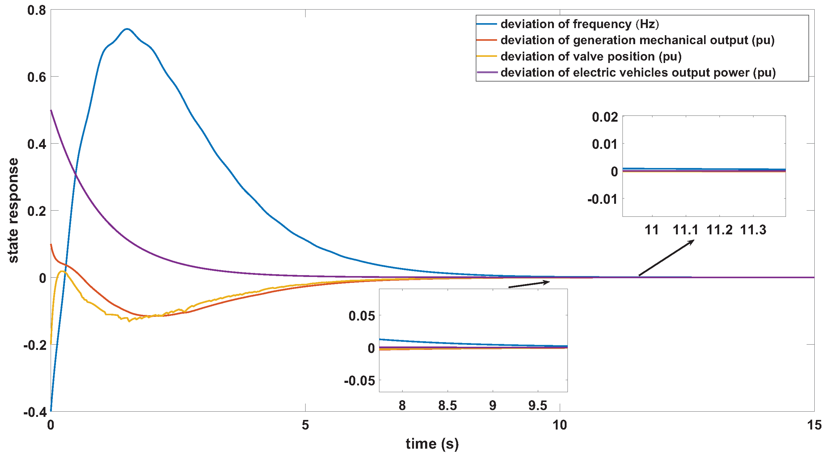
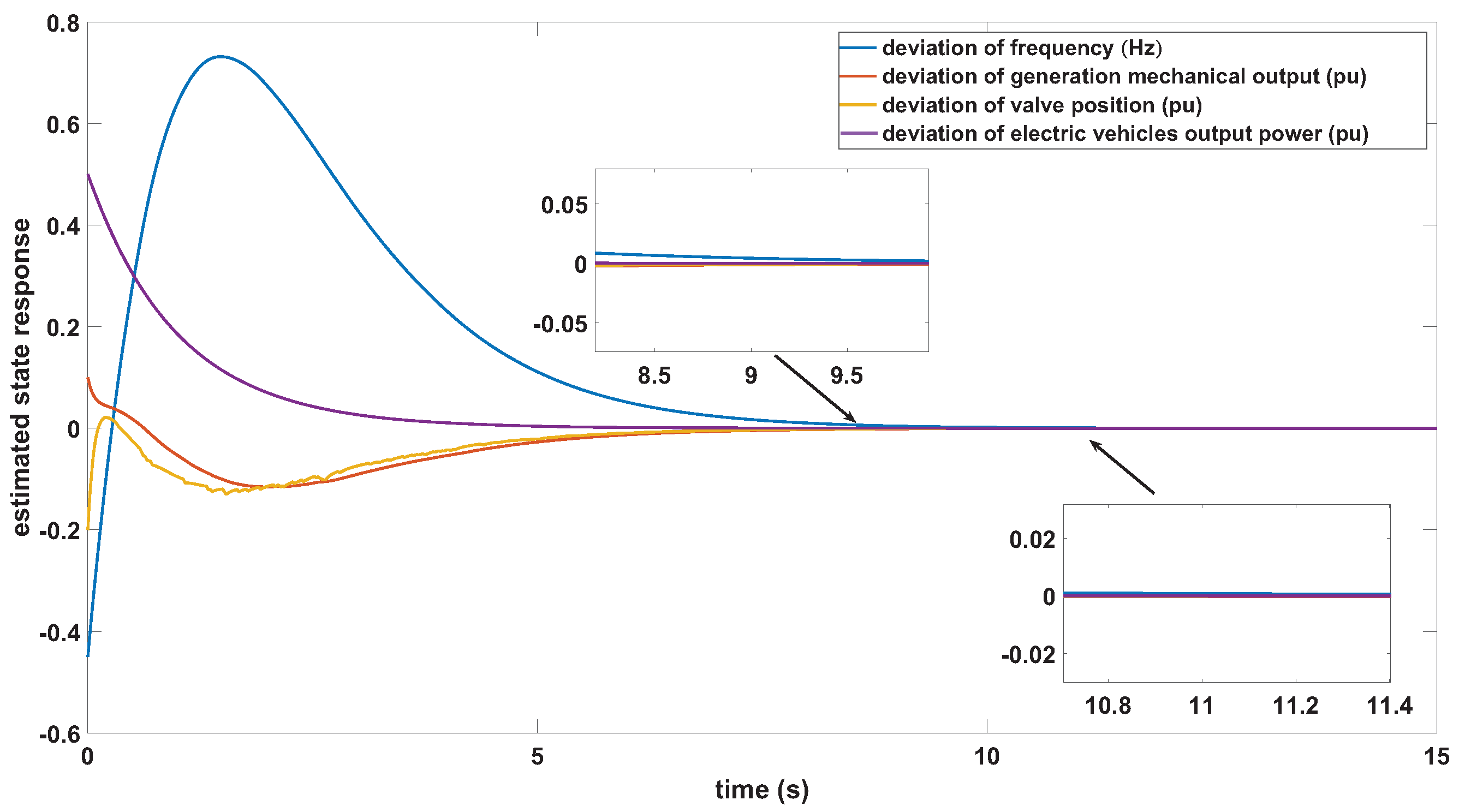
   □
Remark 5.
Compared to past associated studies, the main challenge in controller design is to handle the nonlinear terms P 1 B K and P 2 L D . We make P 1 B K = B Y and P 2 L D = G D by introducing matrices Y and G of suitable dimensions. To ensure the  H performance of cyber power systems, we give normal LMI conditions to design the observer-based feedback controller (9), which can be addressed by the LMI control toolbox.

4. A Case Study

In the part, we show that the theoretical results achieved can be used to solve the LFC problem for power systems with multi-path missing measurements and input–output time-varying delays as well as cyber attacks in the communication channels with the help of an example. Table 2 shows the parameter values for system (9).
Let the probability of the three Bernoulli stochastic variables as α = 0.9 , β = 0.9 , and θ = 0.1 . Time delays are set as  ϑ ( t ) = 0.1 + 0.1 sin ( t ) , H performance index is set as  γ = 7, and the noise signal is selected as  w ( t ) = 0.1 sin ( 4 π t ) 1 + t 2 ( ε ( t ) ε ( t 5 ) ) . Next, using Algorithm 1, the controller gains matrix K and observer gains matrix L, and can be solved as follows:
K = 0.0391 0.0038 0.0032 0.0224 ,
L = 2.1054 0.2981 0.4177 0.0568 T .
Algorithm 1: Load frequency controller and observer design for networked power systems
  • Require: T c h , T g , R, D, M, β , T e , k e , E { α ( t ) } , E { β ( t ) } , E { θ ( t ) } , α g , α e , ϑ M , κ and μ
  • Ensure: The given parameters are reasonable in describing multi-area power systems  
  • 1: Computing the matrices A, B, C and D in system Figure 1 using the input parameters.
  • 2: Solving linear matrix inequalities (24) and (25) in theorem 2 using LMI toolbox.  
  • 3: Obtaining matrices P 1 , P 2 , G and Y.  
  • 4: Calculating K = ( B T P 1 B ) 1 B T B Y ; return K;  
  • 5: Calculating L = P 2 1 G ; return L;
Suppose that cyber attacks signal f ( x ( t ϑ ( t ) ) ) = t a n h ( 0.05 x ( t ϑ ( t ) ) ) , then it is easy to see that H = 0.05 satisfies Hypothesis 1. For the sake of simulation, the initial conditions for the state is selected as x ( 0 ) = 0.4 0.1 0.2 0.5 T and the sampling period is set by 0.01 s and the simulation time is set to 15 s. Figure 3 depicts the Bernoulli distribution for the case of random variables α ( t ) , β ( t ) , and θ ( t ) with expectation α = 0.9, β = 0.9, and θ = 0.1. The α = 0.9 , β = 0.9 , and θ = 0.1 in Figure 3 indicate that 10 percent of the packets from the sensor to the controller are lost, 10 percent of control input packets are lost in the communication network from the controller to the actuator, and the probability of a deception attack in the communication network is 10 percent. Frequency deviation curves of the system and the observer are shown in Figure 4 when the system is subject to packet loss and spoofing attacks. From Figure 4, it can be concluded that the frequency deviation in the power system tends to zero at around 11 s, proving the effectiveness of the designed controller. Figure 5 shows the error between the system frequency deviation and the frequency deviation observed by the observer. Combining Figure 4 and Figure 5, we can see not only that the observer can observe the frequency deviation of the system very well but also that the error between the system frequency deviation and the observed frequency deviation of the observer tends to zero at around 8 s, demonstrating the good observational performance of the designed observer.
Figure 6, Figure 7, Figure 8 and Figure 9 show all state trajectory, all state observation trajectory, systems error trajectory, and the control trajectory of the one-area power system. It is clear from Figure 6 and Figure 7 that system (9) reaches mean square asymptotic stability within 12 s by designing controller (5). We can see that the error between the system state and the observed state of the observer converges to zero around 8 s from Figure 8, which proves that the designed observer (7) is capable of observing the actual value effectively. The control signal u(t) is shown in Figure 9. The disturbance signal is depicted in Figure 10. Figure 11 depicts the response curve of the network attack signal f ( x ( t ϑ ( t ) ) ) . The results show that the presented LFC strategy is able to keep the stability of power systems in the presence of multi-path missing measurements and input–output time-varying delays as well as cyber attacks on the communication channels.

5. Conclusions

This paper is dedicated to studying the mean square asymptotic stability as well as H performance of networked power systems with multi-path missing measurements and input–output time-varying delays as well as cyber attacks on the communication channels. An observer-based LFC model for networked power systems is established, which not only takes into account multi-path missing measurements and input–output time-varying delays in the communication channel but also considers the influences of random cyber attacks on data transmission. Based on this model, with the help of Lyapunov stability theory and LMI techniques, we derived sufficient conditions for the stability and H performance of the system. The validity of the proposed solution is verified by means of simulation examples. It should be noted that we extended the model to a practical situation comparing with previous works due to the frequently occurrence of packet dropouts and cyber attacks phenomenon since it may diminish system performance; however, the approach proposed in this paper also has the following limitations:
Firstly, we model the loss of packets and the occurrence of cyber attacks as Bernoulli stochastic processes, which are somewhat limited in practical applications. Secondly, the stability criterion obtained from the generalized function chosen in this paper is somewhat conservative when dealing with time delay systems. In the future, the simultaneous consideration of input and output packet dropouts described by other efficient stochastic processes and time-varying signal delays deserves further study.

Author Contributions

Y.G., G.L. and J.S. contributed to developing the ideas of this research, Y.G., G.L., G.Z. and H.L. performed the research. All of the authors were involved in preparing this manuscript. All authors have read and agreed to the published version of the manuscript.

Funding

This work was supported in part by the National Natural Science Foundation of China under Grant 62003168, Natural Science Foundation of Jiangsu Province under Grant BK20210569, and Natural Science Research Project of Jiangsu Higher Education Institutions under Grant 20KJB120003, 20KJB470025.

Data Availability Statement

Data sharing not applicable to this article as no datasets were generated or analyzed during the current study.

Conflicts of Interest

The authors declare no conflict of interest.

References

  1. Wu, Z.; Mo, H.; Xiong, J.; Xie, M. Adaptive event-triggered observer-based output feedback L load frequency control for networked power systems. IEEE Trans. Ind. Inform. 2019, 16, 3952–3962. [Google Scholar] [CrossRef]
  2. Singh, V.; Kishor, N.; Samuel, P. Load frequency control with communication topology changes in smart grid. IEEE Trans. Ind. Inform. 2016, 12, 1943–1952. [Google Scholar] [CrossRef]
  3. Jiang, L.; Yao, W.; Wen, J.; Chen, S.; Wu, Q. Delay-dependent stability for load frequency control with constant and time-varying delays. IEEE Trans. Power Syst. 2012, 27, 932–941. [Google Scholar] [CrossRef]
  4. Zhang, Y.; Li, X. A note on L2-gain analysis for power systems with delayed load frequency control schemes. J. Frankl. Inst. 2021, 358, 7586–7602. [Google Scholar] [CrossRef]
  5. Zhang, H.; Liu, J.; Xu, S. H load frequency control of networked power systems via an event-triggered scheme. IEEE Trans. Ind. Electron. 2020, 67, 7104–7113. [Google Scholar] [CrossRef]
  6. Zhang, Y.; Yang, T. Decentralized switching control strategy for load frequency control in multi-area power systems with time delay and packet losses. IEEE Access 2020, 8, 15838–15850. [Google Scholar] [CrossRef]
  7. Pradhan, S.; Das, D. H controller design for frequency control of delayed power system with actuator saturation and wind source integration. Arab. J. Sci. Eng. 2022, 67. [Google Scholar] [CrossRef]
  8. Feng, W.; Xie, Y.; Luo, F.; Zhang, X.; Duan, W. Enhanced stability criteria of network-based load frequency control of power systems with time-varying delays. Energies 2021, 14, 5820. [Google Scholar] [CrossRef]
  9. Zhao, F.; Yuan, J.; Wang, N.; Zhang, Z.; Wen, H. Secure load frequency control of smart grids under deception attack: A piecewise delay approach. Energies 2019, 12, 2266. [Google Scholar] [CrossRef] [Green Version]
  10. Zhao, X.; Zou, X.; Wang, N.; Zhong, M. Decentralized resilient H load frequency control for cyber-physical power systems under DoS attacks. IEEE/CAA J. Autom. Sin. 2021, 8, 1737–1751. [Google Scholar] [CrossRef]
  11. Fayek, H. 5G Poor and Rich Novel Control Scheme Based Load Frequency Regulation of a Two-Area System with 100% Renewables in Africa. Fractal Fract. 2021, 5, 2. [Google Scholar] [CrossRef]
  12. Zhang, C.; Jiang, L.; Wu, Q.; He, Y.; Wu, M. Delay-dependent robust load frequency control for time delay power systems. IEEE Trans. Power Syst. 2013, 28, 2192–2201. [Google Scholar] [CrossRef]
  13. Sargolzaei, A.; Kang, K.; Lghani, M.; Mehbodniya, A.; Sargolzaei, S. A novel technique for detection of time delay switch attack on load frequency control. Intell. Control Autom. 2015, 6, 205–214. [Google Scholar] [CrossRef]
  14. Pradhan, S.; Das, D. H load frequency control design based on delay discretization approach for interconnected power systems with time delay. J. Mod. Power Syst. Clean Energy 2021, 9, 1468–1477. [Google Scholar] [CrossRef]
  15. Sun, Y.; Wang, Y.; Wei, Z.; Sun, G.; Wu, X. Robust H load frequency control of multi-area power system with time delay: A sliding mode control approach. IEEE/CAA J. Autom. Sin. 2018, 5, 610–617. [Google Scholar] [CrossRef]
  16. Ahuja, A.; Narayan, S.; Kumar, J. Two degrees of freedom observer controller for load frequency control with communication delay. J. Control Instrum. 2017, 8, 35–44. [Google Scholar]
  17. Wang, Y.; Yan, W.; Zhang, H.; Xie, X. Observer-based dynamic event-triggered H LFC for power systems under actuator saturation and deception attack. Appl. Math. Comput. 2022, 420. [Google Scholar] [CrossRef]
  18. Sathishkumar, M.; Liu, Y. Resilient annular finite-time bounded and adaptive event-triggered control for networked switched systems with deception attacks. IEEE Access 2021, 9, 92288–92299. [Google Scholar] [CrossRef]
  19. Tian, E.; Peng, C. Memory-based event-triggering H load frequency control for power systems under deception attacks. IEEE Trans. Cybern. 2020, 50, 4610–4618. [Google Scholar] [CrossRef]
  20. Shen, Z.; Yang, F.; Chen, J.; Zhang, J.; Hu, A.; Hu, M. Adaptive event-triggered synchronization of uncertain fractional order neural networks with double deception attacks and time-varying delay. Entropy 2021, 23, 1291. [Google Scholar] [CrossRef]
  21. Tapin, L.; Mehta, R. An integral with feed forward control for primary load frequency control loop using pole-placement design. Int. J. Electr. Electron. Data Commun. 2014, 2, 38–45. [Google Scholar]
  22. Vrdoljak, K.; Peri, N.; Petrovi, I. Sliding mode based load-frequency control in power systems. Electr. Power Syst. Res. 2010, 80, 514–527. [Google Scholar] [CrossRef]
  23. Fernando, T.; Emami, K.; Yu, S.; Iu, H.; Wong, K. A novel quasi-decentralized functional observer approach to LFC of interconnected power systems. IEEE Power Energy Soc. Gen. Meet. 2016, 31, 3139–3151. [Google Scholar]
  24. Pham, T.; Trinh, H.; Le, V. Load frequency control of power systems with electric vehicles and diverse transmission links using distributed functional observers. IEEE Trans. Smart Grid 2015, 7, 238–252. [Google Scholar] [CrossRef]
  25. Wang, Z.; Liu, Y.; Yang, Z.; Yang, W. Load Frequency Control of Multi-Region Interconnected Power Systems with Wind Power and Electric Vehicles Based on Sliding Mode Control. Energies 2021, 14, 2288. [Google Scholar] [CrossRef]
  26. Liu, J.; Gu, Y.; Zha, L.; Liu, Y.; Cao, J. Event-triggered H load frequency control for multiarea power systems under hybrid cyber attacks. IEEE Trans. Syst. Man Cybern. Syst. 2019, 49, 1665–1678. [Google Scholar] [CrossRef]
  27. Wang, J.; Xia, J.; Shen, H.; Xing, M.; Park, J. H synchronization for fuzzy Markov jump chaotic systems with piecewise-constant transition probabilities subject to PDT switching rule. IEEE Trans. Fuzzy Syst. 2021, 29, 3082–3092. [Google Scholar] [CrossRef]
  28. Liu, J.; Wu, Z.; Yue, D.; Park, J. Stabilization of networked control systems with hybrid-driven mechanism and probabilistic cyber attacks. IEEE Trans. Syst. Man Cybern. Syst. 2021, 51, 943–953. [Google Scholar] [CrossRef]
  29. Yan, H.; Zhang, H.; Zhan, X.; Li, Z.; Yang, C. Event-based H fault detection for buck converter with multiplicative noises over network. IEEE Trans. Circuits Syst. Regul. Pap. 2019, 66, 2361–2370. [Google Scholar] [CrossRef]
  30. Tian, E.; Wang, K.; Zhao, X.; Shen, S.; Liu, J. An improved memory-event-triggered control for networked control systems. J. Frankl. Inst. 2019, 356, 7210–7223. [Google Scholar] [CrossRef]
  31. Zhou, Q.; Shi, P.; Xu, S.; Li, H. Observer-based adaptive neural network control for nonlinear stochastic systems with time delay. IEEE Trans. Neural Netw. Learn. Syst. 2013, 23, 71–80. [Google Scholar] [CrossRef] [PubMed]
  32. Yan, H.; Su, Z.; Zhang, H.; Yang, F. Observer-based H control for discrete-time stochastic systems with quantisation and random communication delays. IET Control. Theory Appl. 2013, 7, 372–379. [Google Scholar] [CrossRef]
  33. Zhao, Y.; Duan, Z.; Wen, G.; Zhang, Y. Distributed finite-time tracking control for multi-agent systems: An observer-based approach. Syst. Control Lett. 2013, 62, 22–28. [Google Scholar] [CrossRef]
  34. Tan, F.; Zhou, L. Analysis of random synchronization under bilayer derivative and nonlinear delay networks of neuron nodes via fixed time policies. ISA Trans. 2022. [Google Scholar] [CrossRef] [PubMed]
Figure 1. System LFC model including electric vehicles.
Energies 15 04234 g001
Figure 2. Structure of networked power systems with limited communications and cyber attacks.
Energies 15 04234 g002
Figure 3. The evolution of the Bernoulli stochastic variables with α = 0.9, β = 0.9, and θ = 0.1.
Energies 15 04234 g003
Figure 4. Frequency deviation Δ f and estimated frequency deviation Δ ^ f .
Energies 15 04234 g004
Figure 5. Error in frequency deviation between the system and observer.
Energies 15 04234 g005
Figure 6. State trajectory of one-area power system.
Energies 15 04234 g006
Figure 7. Observation trajectory of one-area power system.
Energies 15 04234 g007
Figure 8. Error trajectory of one-area power system.
Energies 15 04234 g008
Figure 9. Control input trajectory of one-area power system.
Energies 15 04234 g009
Figure 10. The response of disturbance signal.
Energies 15 04234 g010
Figure 11. The response of deception attacks signals.
Energies 15 04234 g011
Table 1. Networked power systems parameters and their names.
SymbolName
Δ f 
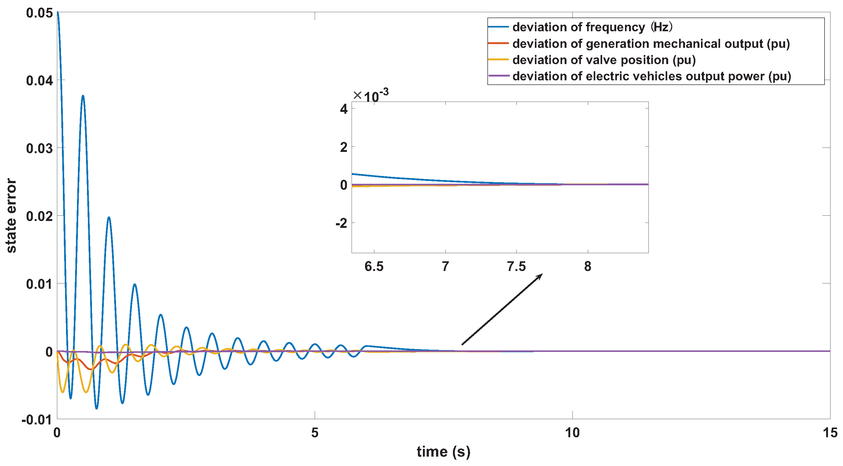
the deviations of frequency
Δ P m the deviations of generation mechanical output
Δ P v the deviations of valve position
Δ P d the deviations of load
Δ P e the deviations of electric vehicles output power
A C E ( t ) area control error
Mthe moment of inertia of the generator
Dthe generator damping coefficient
T g the time constant of the governor
T c h the time constant of the turbine
T e the time constant of the electric vehicles
Rthe speed drop
α g turbine proportionality factor
α e electric vehicles proportionality factor
β the frequency bias factor
k e electric vehicles gain factor
Table 2. Power Systems Parameters for LFC [25].
T ch T g RDM β T e k e α g α e
0.30.10.051100.4110.90.1
Publisher’s Note: MDPI stays neutral with regard to jurisdictional claims in published maps and institutional affiliations.

