Energy Efficient UAV Flight Control Method in an Environment with Obstacles and Gusts of Wind

Abstract

This article presents an energy-efficient method of controlling unmanned aircraft (fixed-wing UAVs), which consists of three groups of algorithms: aerial vehicle route planning, in-flight control, and algorithms to correct the preplanned flight trajectory. All algorithms shall take into account the existence of obstacles that the UAV must avoid and wind gusts in the UAV’s area of operation. Tests were carried out on the basis of the UAV mathematical model, stabilization and navigation algorithms, and Dryden turbulence model, considering the parameters of the UAV’s propulsion system. The work includes a detailed description of constructing a network of connection that is used to plan a UAV mission. It presents the algorithm for determining the actual distances between the different points in the field of action, which takes into account the existence of obstacles. The algorithm shall be based on methods for determining the flight trajectory on a hexagonal grid. It presents the developed proprietary UAV path planning algorithm based on a model from a group of algorithms of mixed integer linear problem (MILP) optimization. It presents the manner in which the pre-prepared flight path was used by UAV controllers that supervised the flight along the preset path. It details the architecture of contemporary unmanned aerial vehicles, which have embedded capability to realize autonomous missions, which require the integration of UAV systems into the route planning algorithms set out in the article. Particular attention has been paid to the planning and implementation methods of UAV missions under conditions where wind gusts are present, which support the determination of UAV flight routes to minimize the vehicle’s energy consumption. The models developed were tested within a computer architecture based on ARM processors using the hardware-in-the-loop (HIL) technique, which is commonly used to control unmanned vehicles. The presented solution makes use of two computers: FCC (flight control computer) based on a real-time operating system (RTOS) and MC (mission computer) based on Linux and integrated with the Robot Operating System (ROS). A new contribution of this work is the integration of planning and monitoring methods for the implementation of missions aimed at minimizing energy consumption of the vehicle, taking into account wind conditions.

1. Introduction

Many authors weigh in on the architecture of modern unmanned flying vehicles [1]. Researchers and constructors agree that any unmanned vehicle that is capable of operating autonomously must be equipped with two types of control units: an FCC (flight control computer) and an MC (mission computer) [2]. The FCC acts as an autopilot and executive unit to control the flight between consecutive points. The MC is the unit supervising the correctness of the implementation of the mission plan. Both of these devices work together in the course of the vehicle’s flight. The article focuses on tasks related to the implementation of a reconnaissance mission by unmanned vehicle equipped with EO/IR sensor and SAR radar. We present a description of the planning and implementation of the reconnaissance mission realized for a single unmanned vehicle, although the model can be used for planning missions for drone swarms. We assume that the mission plan, consisting of the flight path and the payload, is prepared at the ground control station (GCS) before the mission. This plan is then transmitted to the UAV for its computers (FCC under MC supervision) to perform it during the flight (in aviation this is described as the UAV operating autonomously). In some situations, the UAV must modify the flight plan by itself. This is achieved, for example, when there is no contact with GCS when algorithms in the MC confirm the inability to perform the entire planned task. In such a situation, computers must be present on the aerial vehicle which will be able to develop a new flight and payload operation plan. In our case, that task falls to the MC. The plans will be transmitted to the FCC which controls the vehicle’s flight. The subject of the article shall be the architecture of such a system, the UAV flight planning and control algorithms, and the principles for integrating individual components into a system capable of realizing a mission autonomously.

The system architecture developed by the authors has been divided into three main components: mission computer (MC), flight control computer (FCC), and wireless communication subsystems (WCS). The article does not deal with the communication subsystem. Human-Machine-Interface (HMI) is a dedicated software for managing the unmanned system located at the ground control station (GCS). Mission planning usually consists of two variants—loading a pre-prepared mission from a file, or entering individual route points and payload functions manually by the pilot/operator. Regardless of the option, it is always a person who prepares a mission plan. In every unmanned system, the operator may take account of field obstacles, flight zones, etc., by manually adding additional route points which the UAV is only to fly through to arrive at the site of the reconnaissance mission and avoid the obstacle. However, given that the UAV often carries out missions autonomously or in areas with a large number of obstacles, the pilot is forced to manually input many less important route points that are less significant from the perspective of the reconnaissance mission. Therefore, it has been decided to automate the process of modifying the mission in order to avoid obstacles in the proposed solution. Thanks to the algorithm developed, the pilot needs only to input key routing points, and it is the MC’s task to modify the flight path in a manner that allows safe execution of the reconnaissance mission on the basis of geodetic data (or obstacle data sent by the reconnaissance services), external sensor data, or other onboard information. This means that the ground control station’s mission plan, which consists of a UAV route plan and a payload operation plan, is maintained in the MC. The route currently implemented and the emergency return routes are maintained in the FCC, which is the unit responsible for the execution of the flight along the programmed points. MC may, where justified, modify the current flight plan. Descriptions of situations where the MC modifies the flight plan are beyond the scope of the article (some examples are shown in [3]). The modified route plan shall be sent to the FCC. This is specific to situations of lack of communication with the GCS.

The basic control element of the vehicle is the FCC operating in real time with the use of a dedicated real-time operating system (RTOS). RTOS is responsible for the management of threads/tasks and, above all, allows the prioritization of individual tasks. The thread responsible for controlling the vehicle is assigned the highest priority and its diagram is shown in Figure 1.

Figure 1. Unmanned aerial vehicle architecture diagram.

The high-level controller comprises three main subsystems:

(1)

Vehicle stabilization—algorithms based on PID controllers that aim to stabilize the angular position of the UAV in space.

(2)

Stabilization and control of height, vertical speed, and vehicle flight speed—these algorithms were also based on PID controllers supported by state machines and mathematical algorithms based on energy estimation.

(3)

Navigation algorithms—heading control, flight along a required route, loiter, etc. These algorithms were also based on PID controllers supported by mathematical algorithms and input/output signal shaping systems.

The high-level controller shall find and deliver signals to efficient attitude and altitude UAV control, including the propulsion system on the basis of the values set and appointed by the state observer so that the vehicle achieves the preset flight parameters. At this point, it is worth noting that UAVs are specific aerial vehicles with a low altitude variation profile. This implies that the change in altitude is linked to high energy expenditure, which is not recommended for vehicles of this type. An example flight profile is shown in Figure 2.

Figure 2. Example flight profile.

The low-level controller is responsible for transforming signals generated by the high-level controller from angular values, percentages to appropriate hardware values enabling the control of servos, engine controllers, or other actuators. In the presented architecture, the mission computer is based on Robot Operating System (ROS). Flight trajectory determination algorithms are supported by geodetic data (altitude grids), other reconnaissance data, and external sensors. ROS is a dedicated set of libraries and software to create robotics software. It allowed for the software architecture within the presented architecture to be divided into smaller modules, so-called nodes. ROS allows to control nodes and for them to communicate with each other, which significantly simplified the development of the software. Mission planner determines the sequence of the UAV flight between the subsequent points along the route. During the planning process, the mission planner considers basic information on the area of operation, including the location of obstacles in the field and the direction and speed of wind. The GCS may additionally use data from the weather forecast. During the flight, the UAV already has accurate wind direction and speed data specified by the air data computer (ADC). Mission planner may correct a predefined route. The trajectory planner is a module that determines the actual distances between the points to which the UAV is flying. The module calculates flight trajectory between any pair of points in the field based on the position of obstacles and the margin to be taken into account so as not to expose the UAV to the risk of destruction. The latter is particularly important in the case of military vehicles. The presented version of the flight trajectory planning module between two points in the field operates on a hexagonal grid, which allows fast trajectory planning and ensures the determination of gentle mid-air turns.

The article presents several innovations and new contributions from the area of algorithm design for fixed-wing UAV flight planning and control. The most important contributions are:

(a)

Planning and adjustment of algorithms of individual flight sections, considering the occurrence of obstacles and tasks related to terrain scanning, are integrated within aerial vehicle control algorithms, which allow for rapid corrections of the designated route plans.

(b)

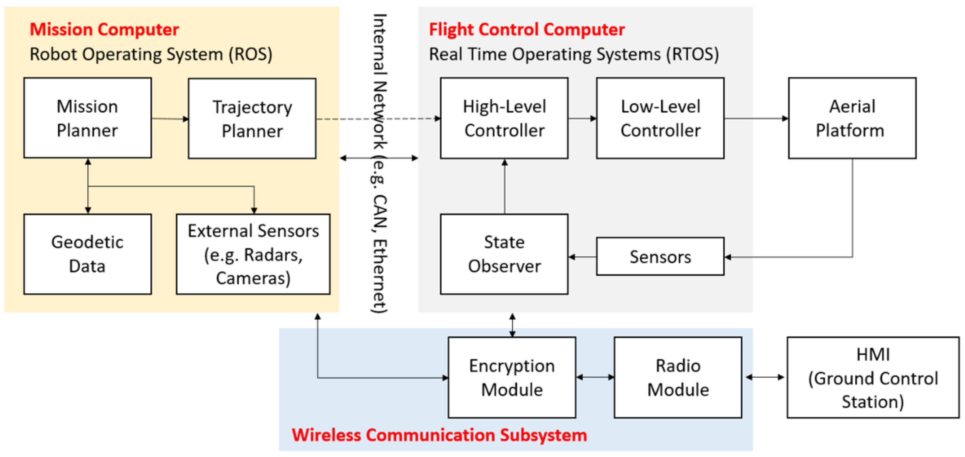
All algorithms were designed in such a way that they could be implemented on vehicles based on ARM architecture, which is the basic architecture of the contemporary UAV—the model-based design technology dedicated by DO-178C and DO-331, DO-332, DO-333 [4,5,6] was used, the MC was based on ROS and the FCC, on RTOS.

(c)

Hexagonal grid-based trajectory determination algorithms used are deterministic, fast, and reliable, which is relevant for the certification thereof by institutions that allow UAVs to operate in controlled airspace.

(d)

All algorithms shall consider the presence of non-zero speed winds.

(e)

Vehicle control algorithms shall take into account wind gusts in accordance with the methodologies described in NATO standards.

(f)

The UAV architecture has been presented, which allows for the execution of autonomous missions, where the planning algorithms described are an important component of the implementation of the mission.

(g)

Hardware-in-the-loop tests were performed.

The remainder of the article presents the following elements. The Related Works chapter presents works related to land modeling for the purpose of determining UAV flight routes and selected algorithms from this area that concern route planning and UAV control. The Models and Methods chapter presents the mathematical model of fixed-wing UAV and the stabilization and navigation algorithms, for which methods for determining and correcting vehicle flight path plans are developed. The following section of the chapter discusses the method for planning and correcting routes simplifying the UAV control process and the way in which route planning models are integrated with UAV controllers. The range of possible interference with FCC control by the MC is discussed in two specific cases: SAR radar reconnaissance flights and reconnaissance in conditions with gusts of wind. For both cases, it was demonstrated how the MC influences the operation of PID controllers that are part of the FCC. The Results chapter presents the results obtained by authors for the unmanned vehicle presented in the article. The Conclusions chapter summarizes the results achieved.

2. Related Works

Sanchez et al. [1] and Boubeta-Puig et al. [7] present the overall construction of an unmanned autonomous system which allows the UAV to change the trajectory in the absence of GCS control. The system consists of several modules, depending on its intended use, responsible for the implementation of the mission plan in autonomous mode (without contact with GCS). Another example of UAV avionic equipment architecture is presented by Ilarslan et al. in [8]. In this approach, the MC acts as the main control system and is therefore based on the RTOS, with the FCC autopilot being a slave system. It uses generally CAN and RS232 interfaces.

FCC is equipped with a state machine with an embedded logic of special and emergency situations which enables it to determine incorrect operation of the MC on its own. Therefore, the MC could be developed on the Robot Operating System open-source software [9]. ROS is widely applicable in robotics, allows for a division of an entire system into individual nodes, which makes the addition of new functionalities much easier. MC is equipped with mission planning software that takes into account the performance of the payload and supports FCC, thus making it possible to make optimal use of UAV capabilities for its mission. Descriptions of the elements of the state machines implemented on computers of the aerial vehicle can be found in [3,10,11].

In many works, where an additional computer is used, which acts as a calculation unit, e.g., to navigate obstacles, modify flight paths, and other additional functions, ROS (Robot Operating System) is used. In the work of Yu et al. [12], a commercial UAV was used, which was connected to a computer based on ROS to control the UAV using predefined human gestures. A similar approach was presented by Carvalho et al. [13], where the PX4—FCC open-source autopilot was combined with a computer with Linux and ROS. In addition, ROS is often used for prototyping mission planning algorithms and testing them in a virtual 3D environment (Zhang et al. [14]). Having analyzed the abovementioned works, it can be concluded that the vast majority of them use ROS for an additional/external computer. The FCC is responsible for the basic functions of stabilization and control and is able to operate independently of the mission computer that plays a supporting role. Communication between FCC and MC uses network interfaces equipped with a sensor system. Such a connection shall allow direct access to data of both FCC and MC.

The integration of FCC and MC may involve the exchange of information of two types. First, the MC may send a correction of the mission plan to the FCC when the MC’s analyses show that, as a result of changes in weather conditions, the UAV is unable to perform the task within the time frame set. In such a case, MC modules set out a mission correction by solving VRPTW optimization tasks shown, for example, in [15] or [16]. The second type of integration is the impact on the current FCC control in order to run a certain behavior of the aerial vehicle. For example, in order to correctly scan the area using SAR radar, it is important that the UAV does not exceed the maximum roll angle in spite of desired path, as described in [16]. In this case, FCC mechanisms must respond to MC control signals and block the operation of the standard controller, as shown in the article.

In order for the FCC to be able to receive a modified mission plan designated by the MC, the MC needs first to have a model of the area where the operation is to be carried out. Land models used to represent the UAV area of operations are directly conditional on the types of algorithms that can be used for mission planning and flight trajectory determination. The article is based on a model of a grid of connections in the form of a graph built before the mission planning task is solved (see Figure 3). From a formal point of view, a grid is constructed, S the edges of which model UAV flight sections and the vertices model locations where flight parameters of the unmanned system or equipment are changed. At the area modeled with a vertex, it is also possible to identify a small object. However, there is a presumption that the grid itself is not changed in the process of determining the solution, i.e., mission plan development. In case of new obstacles, the grid may be modified and the algorithm itself restarted. The key aspect here is the grid design algorithm for $S=<G,\mathsf{\Phi },\mathsf{\Psi }>$, where G means a consistent graph within the meaning of the graph and grid theory, $\mathsf{\Phi }$ means a set of functions defined at the vertices of the graph, and $\mathsf{\Psi }$ means a set of functions defined on the graph edges. On the edges, the flight path of one or more unmanned vehicles is determined. Several basic network design methods are used for the construction of graph-based networks.

Figure 3. Fragment of a UAV mission plan with marked alternative routes and the object of reconnaissance and danger zone in the form of a grid of connections in the field. The section (k,m) is reconnoitred using the available sensor. An area is marked from where the object to be reconnoitred is visible in the form of a cone with the middle where the target is located (marked with a black triangle). The area covered by the sensor is marked with a dark blue trapeze.

The first, simplest way of constructing a graph modeling potential routes in the area where the vehicle can move around is a square grid. Each square (usually the same size) is the vertex of the grid and is connected to adjacent squares, which is modeled through the edges of the graph. The grid of squares is the most commonly used land model for autonomous vehicle routing [17]. From the perspective of vehicle movement, the construction of such a network seems natural, although recently, more frequent models based on regular hexagons (hexagonal grids) are used, which allows modeling smooth turns for the vehicles [18]. The problem with the use of such land representation is the number of grid vertices created in the planning of the unmanned aerial vehicle mission, which operates over several hundred square kilometers and altitudes between 500 to a few thousand meters above ground level. In such a case, the grid may be constructed from thousands of vertices for which it is necessary to verify whether they are within the mission area, a dangerous area, a safe area, or an other area. Therefore, the article assumes that the UAV flight profile relates to a flight at a specified operating altitude throughout a major part of the mission, which is a correct assumption and most frequent for UAV mission planning. The article presents a method for determining routes between any vertices of a hexagonal grid. This approach, which is increasingly popular in planning the traffic of unmanned systems, has two main advantages: it is very efficient calculation-wise and ensures that turns are defined, which are easy for the UAV to perform.

When analyzing mission planning and flight trajectory designation algorithms, account should also be taken of the used obstacle model affecting the UAV flight. Relevant literature discusses static and dynamic models of objects posing a threat to UAVs (e.g., Wen et al. [19]).

The paper [20] focuses on the constrained control of UAVs in geofencing applications. The constraints defined for the obstacles are vertical infinite cylinders and are located inside the boundaries defined by other constraints. It is demonstrated that the system is effective. The paper shows experiments for a small number of obstacles. For an environment with many obstacles, the number of constraints will be very large. This is why we decided to use a grid-based map of the environment in our system.

In [21] it is assumed that nodes collect the environmental parameters. The data are transferred to the UAV and to the remote base station. The land system computes the UAV’s flying trajectory, and the parameters such as distance and time are taken into account. In our system, we do not have sensors that study environmental conditions, but parameters such as energy consumption and path length can be taken into account.

The article does not deal with the subject of dynamic obstacles. With regard to the use of static obstacle/hazard models, we rely on two basic assumptions. Firstly, the objects threatening the UAV are anti-drone systems of various types, with ranges modeled using a semi-sphere, as shown in Figure 3. Such models work in most applications when we know the risk or at least can presume its type. When we do not know the exact nature of the hazard, we define the area in which it occurs (usually it is convex polygons) and determine the maximum altitude to which the object threatens the aerial vehicle for this area. It is a very practical assumption due to the fact that the majority of UAVs have operational ceilings, in addition to which the cost of the flight is much higher. Moreover, frequent changes in the flight altitude of the platforms significantly reduce their flight duration, so the assumption that obstacles should be circumvented rather than flown over is justified. The article uses a model of obstacles in the form of convex polygons, which does not reduce the general nature of considerations. The presence of obstacles in the field increases the number of grid vertices where mission planning tasks are solved.

Following the designation of the grids of connections, UAV flight routes may be determined. If the literature of the subject regarding the design of heuristic algorithms accelerating the achievement of an acceptable and suboptimal solution for the problem described in the article is analyzed, particle swarm optimization (PSO), genetic algorithms (GA), or their modifications based on the Tabu Search technique (Fu et al. [22]) are the most frequently described in the group of algorithms taking time windows into account, whereas algorithms using Tabu techniques (Lau et al. [23], Gmira et al. [24]) are among the most commonly used. The general principle of operation is to predefine the allowable allocation of tasks to a predetermined number of vehicles so that in subsequent iterations, they attempt to randomly improve the allocation of tasks by replacing one or more tasks assigned to specific vehicles. In order to avoid multiple repetitions of the same movement, a list of prohibited movements is introduced (Tabu list). Different approaches to building the initial solution and exchanging assigned tasks between vertices are introduced in different implementations of this class of algorithms.

The works [25,26] present the application of reinforcement learning and deep learning for UAV control. The use of reinforcement learning is promising, but it is very expensive to test with a real environment. The most important issue in our project is robustness which is why we decided to use a classic PID controller in the current version of our system.

In our work so far, we focused primarily on planning a reconnaissance mission, in particular on determining UAV flight routes and the payload operation plan. To solve the UAV route planning task, we use task scheduling algorithms with time windows (vehicle route planning with time windows—VRPTW) that take into account the specificities of the unmanned vehicle flight. The algorithms presented may be used both in the planning of individual UAV missions and where UAV groups cooperate in multi-agent systems. The approach presented is a practical way of establishing mission plans implemented in actual unmanned systems. A very good overview of algorithms of this type can be found in Zhou et al. [27].

3. Models and Methods

3.1. UAV Mathematical Model

It was necessary to develop a mathematical UAV fixed-wing model. The UAV selected was the AFIT Neox [28]. A simplified model is shown in Figure 4. The figure indicates the reference systems used in the mathematical modeling process and the main actuating systems (electric motor—M and two servos: right—$s_r$ and left—$s_l$).

Figure 4. UAV Neox model.

The mathematical model describes a rigid body dynamics considering forces and moments equation system. The differential equations of kinematic and dynamics of UAV were determined using Newton’s second law of motion. To implement the above-mentioned relationships to the simulation environment, simplifications are performed, neglecting less important phenomena. However, they allow the calculation process to be accelerated.

The following simplification assumptions have been taken into account in the formulation of the UAV mathematical model:

• It is assumed that the object under consideration is rigid, not deformable, of constant weight, and constant inertia.
• The center of mass is fixed and does not change.
• The impact of the Earth’s curvature has been neglected and it has been assumed that the gravity field is homogeneous.
• UAV movement equations were derived from the angular and linear moment change law.

To describe the forces and moments affecting UAVs, frames of reference compliant with PN-ISO 1151 (flight dynamics—concepts, quantities, and symbols) and markings from [PN-ISO 1151] have been adopted. Coordinate systems (Figure 5a,b) are described as follows:

Figure 5. Frames of reference compliant with PN-ISO 1151 describing the forces and moments affecting UAVs. (a) $O{x}_g{y}_g{z}_g$ and $Oxyz$ frames of reference. (b) $O{x}_a{y}_a{z}_a$ and $Oxyz$ frames of reference. $O{x}_a{y}_a{z}_a$ and $Oxyz$ frames of reference.

• $Oxyz$—UAV/body frame.
• $O{x}_g{y}_g{z}_g$ —Earth frame.
• $O{x}_a{y}_a{z}_a$—wind frame.

The transformation matrices between individual frames of reference are shown below:

$$L_{qg}=\left[\begin{array}{ccc}cos\psi ·cos\theta & sin\psi ·cos\theta & -sin\theta \\ cos\psi ·sin\theta ·sin\varphi -sin\psi ·cos\varphi & sin\psi ·sin\theta ·sin\varphi +cos\psi ·cos\varphi & cos\theta ·sin\varphi \\ cos\psi ·sin\theta ·cos\varphi +sin\psi ·sin\varphi & sin\psi ·sin\theta ·cos\varphi -cos\psi ·sin\varphi & cos\theta ·cos\varphi \end{array}\right]$$

(1)

$$L_{qa}=\left[\begin{array}{ccc}cos\alpha ·cos\beta & -cos\alpha ·sin\beta & -sin\alpha \\ sin\beta & cos\beta & 0\\ sin\alpha ·cos\beta & -sin\alpha ·sin\beta & cos\alpha \end{array}\right]$$

(2)

where

$L_{qg}$—transformation matrix between $O{x}_g{y}_g{z}_g$ and $Oxyz$.

$\psi$—yaw angle.

$\theta$—pitch angle.

$\varphi$—roll angle.

$\alpha$—UAV attack angle.

$\beta$—UAV slip angle.

The aeroplane model is described by twelve differential Equations (3)–(12), the solution of which consists of a state vector (13):

$$\dot{U}=\frac{F_x}{m}+rV-qW$$

(3)

$$\dot{V}=\frac{F_y}{m}+pV-rU$$

(4)

$$\dot{W}=\frac{F_z}{m}+qU-pV$$

(5)

$$\dot{p}=\frac{M_x+(I_y-I_z)qr}{I_x}$$

(6)

$$\dot{q}=\frac{M_y+(I_z-I_x)rp}{I_y}$$

(7)

$$\dot{r}=\frac{M_z+(I_x-I_y)pq}{I_z}$$

(8)

$$\dot{\varphi }=p(qsin\varphi +rcos\varphi )tan\theta$$

(9)

$$\dot{\theta }=qcos\varphi -rsin\varphi$$

(10)

$$\dot{\psi }=\frac{rcos\varphi +qsin\varphi }{cos\theta }$$

(11)

$$\left[\begin{array}{c}\dot{x_g}\\ \dot{y_g}\\ \dot{z_g}\end{array}\right]=L_{qg}^{-1}\left[\begin{array}{c}U\\ V\\ W\end{array}\right]$$

(12)

$$X={[U,V,W,p,q,r,\varphi ,\theta ,\psi ,x_g,y_g,z_g]}^T$$

(13)

where

$U,V,W$—linear speeds in the body frame $Oxyz$.

$p,q,r$—angular speeds in the body frame $Oxyz$.

$F_x,F_y,F_z$—forces acting on the object in the body frame $Oxyz$.

$M_x,M_y,M_z$—moments acting on the object in the body frame $Oxyz$.

m –mass of the UAV.

$I_x,I_y,I_z$—moments of inertia of the UAV.

$O{x}_g{y}_g{z}_g$—UAV position in the Earth frame.

For fixed-wing UAVs, the key performance parameters are aerodynamics of the vehicle. Aerodynamic derivatives and dynamic pressure influence aerodynamic forces and moments according to dependencies [10]:

$$F_{x_a}=-C_{x_a}·\frac{\rho |V_{aer}{|}^2}{2}S$$

(14)

$$F_{y_a}=C_{y_a}·\frac{\rho |V_{aer}{|}^2}{2}S$$

(15)

$$F_{z_a}=-C_{z_a}·\frac{\rho |V_{aer}{|}^2}{2}S$$

(16)

$$L_{aer}=-C_l·\frac{\rho |V_{aer}{|}^2}{2}S$$

(17)

$$M_{aer}=C_m·\frac{\rho |V_{aer}{|}^2}{2}S$$

(18)

$$N_{aer}=C_n·\frac{\rho |V_{aer}{|}^2}{2}S$$

(19)

where

$U_{aer}=U-U_{wind}$.

$V_{aer}=V-V_{wind}$.

$W_{aer}=W-W_{wind}$.

$|V_{aer}|=\sqrt{(U_{aer}^2+V_{aer}^2+W_{aer}^2)}$.

$F_{x_a}$—drag force.

$F_{y_a}$—side drag force.

$F_{z_a}$—lift force.

$L_{aer}$—roll moment.

$M_{aer}$—pitch moment.

$N_{aer}$—yaw moment.

According to the above relationships, generated forces and moments strongly depend on aerodynamic speed. Therefore, wind and turbulence parameters have a significant impact on the energy demands for a flight with desired parameters. In addition, the above relations show that if the wind strength will generate too big a drag force, there may be a situation where the aeroplane is unable to generate enough thrust that will enable the UAV to move in the intended direction. In this article, the UAV is equipped with a drive set based on a BLDC electric motor and a two-blade propeller. The drive set is located in the rear part of the UAV.

As part of the implementation of the project by AFIT for State security and defense financed by The National Centre for Research and Development under the code name of “BRUS”, tests have been carried out to determine the characteristics of the propulsion system under flow conditions (Figure 6).

Figure 6. Drive unit set at an angle of 90°in relation to the direction of inflow.

The tests were performed for three dynamic pressure values, q = 200 Pa, q = 300 Pa, and q = 500 Pa, at three angular settings of the drive unit 90°, 30°, and 15°. The dynamic pressures were 18.2 m/s, 22.2 m/s, and 28.7 m/s, respectively. Characteristics were determined using a laboratory station for measurement of the drive unit specially designed and developed as part of the project. The drive unit measurements performed for the angle of inclination 90° (inflow direction in accordance with the axis of the propeller shaft) provided the data necessary to determine the characteristics of the propeller:

1.

Thrust coefficient ($C_t$) in function of (J).

2.

Power coefficient ($C_p$) in function of (J).

3.

Propeller efficiency ($\eta$) in function of (J).

Calculations use the following relations:

$$J=\frac{V}{nD}$$

(20)

$$C_t=\frac{T}{\rho n^2{D}^4}$$

(21)

$$C_p=\frac{P}{\rho n^3{D}^5}$$

(22)

$$P_{out}=TV$$

(23)

$$P_{prop}=M\omega$$

(24)

$$\eta =\frac{P_{out}}{P_{prop}}$$

(25)

where

• $C_t$—thrust coefficient.
• $C_p$—power coefficient.
• T—thrust (N).
• $\rho$—air density (kg/m³).
• $\eta$—propeller rotations (rps).
• D—propeller diameter (m).
• J—propeller advance ratio.
• V—airspeed (m/s).
• $P_{out}$—power converted into thrust by the propeller T (N) at speed V (m/s).
• M—moment on the propeller shaft.
• $\omega$—propeller rotation speed (1/s).

Geometric parameters of the propeller used:

• Diameter—0.304 m (measured).
• Pitch—0.102 m (according to manufacturer data).
• H/D—0.336.

It can be noted that the tested drive unit has a relatively low efficiency (Figure 7). This is due to the fact that the tests were carried out for a propeller dedicated for a VTOL craft. The higher the airspeed, the lower the efficiency. Therefore, the UAV drive can be optimized in relation to the minimum and maximum speeds. Conversely, in order to achieve maximum performance, wind direction and speed and flight speed should be taken into account in the planning of the mission.

Figure 7. Diagram of the efficiency of the propeller used in measurements as a function of propeller advance ratio.

The model inputs such as object mass, inertia moments, propulsion system parameters and models, and aerodynamic derivatives were determined analytically and experimentally during the autopilot construction project.

The UAV mathematical model was implemented in the Matlab/Simulink, which includes the following subsystems:

• Standard atmosphere model [29].

–  Dryden wind and turbulence model [30].

• On-board sensor simulator: GPS, IMU, magnetometer, LIDAR, and battery.
• Models of selected elements of mechanical equipment.

A model completed thus was adapted in accordance with the model-based design methodology using reference models [31] for automatic generation of code C per real-time ARM processor. This model is a reference that is used by the control algorithms. Below are the input and output signals of the implemented model. The main control signals are

• Throttle—value of electrical control signal in the range from 0 to 100
• Bh—angular value of the elevator.
• Ba—angular value of the ailerons.

The model so prepared was used to develop and test control and navigation algorithms.

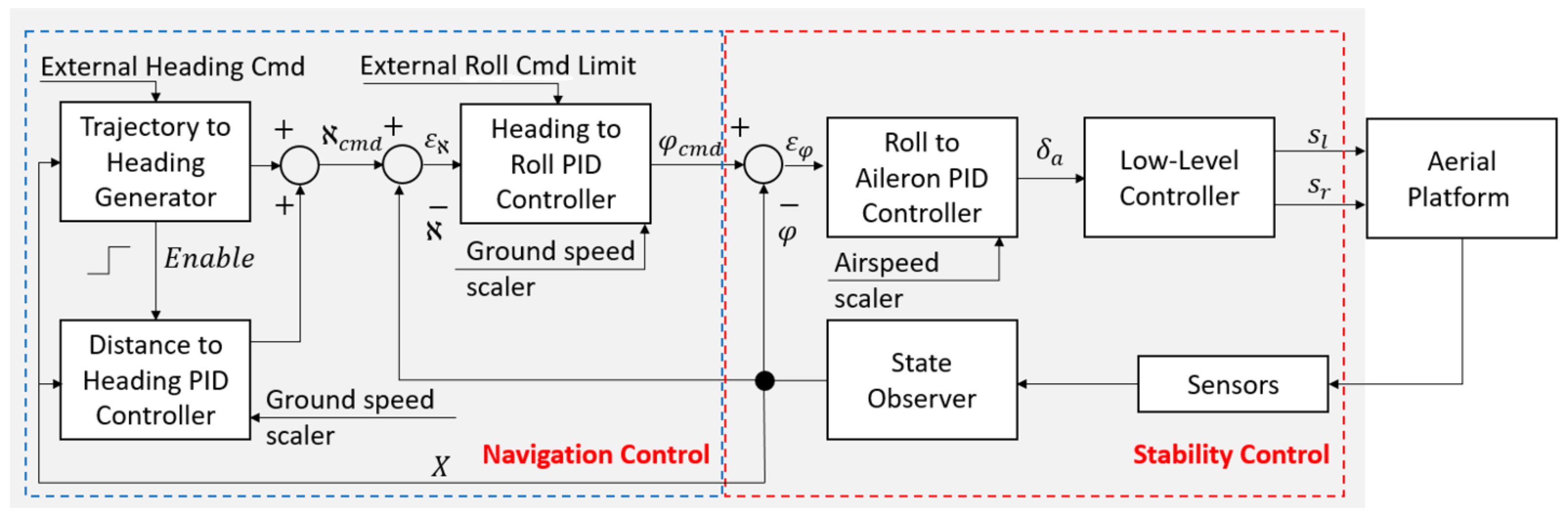
3.2. Stabilization and Navigation Algorithms

The aircraft’s waypoints navigation consists of the continuous control of its course. The course change is carried out by changing the aircraft bank angle. Additionally, a distinction is made between flight to a point and flight along a given path. The above-mentioned tasks are performed by the high-level controller. The high-level controller is based on a cascade connection of the PID controller in accordance with the following block diagram.

Stability control ensures that desired roll angle is maintained regardless of external disturbances. The internal controller shown in Figure 8 ensures transverse stability of the vehicle—stabilization of the roll angle. According to the aerodynamic derivative analysis and the relationship between the dynamic pressure variation proportional to the squared aerodynamic speed, it is necessary to scale (change the operating point) the PID regulator using the parameter airspeed scaler, which is designed to provide controller stability within the full UAV flight speed range. The ${\varphi }_{cmd}$ value and $\varphi$ determined ${ϵ}_{\varphi }$, which defines the error in the roll channel. Subsequently, on the basis of the deviation, the controller sets the angle ${\sigma }_a$ of the ailerons, which the low-level controller converts to the electrical value of the left and right servos $(s_l,s_r)$.

Figure 8. UAV controller block diagram.

The navigation control block consists of a combination of two PID controllers and a heading generator that can take values from an external/master device, e.g., mission computer. The heading to roll PID controller is responsible for maintaining the set course (${\chi }_{cmd}$) by determining the correct value of the ${\varphi }_{cmd}$. This subsystem takes into account the possibility of receiving an external limitation of the ${\varphi }_{cmd}$ output, which enables the flight with low values of the roll angle at the expense of reducing the maneuverability of the aircraft. The trajectory to heading generator is responsible for determining the ${\chi }_{cmd}$ based on the current geographical position of the platform and the destination point. When the ${\chi }_{cmd}$ is determined by the mission computer, the trajectory to heading generator subsystem is omitted and the target course is transmitted through a separate parameter—external heading Cmd. The course determined in this way allows only a flight towards the point; however, it does not allow for a flight along a given path. For this purpose, the distance to heading PID controller is used. This subsystem is triggered from the trajectory to heading generator to improve maneuverability. Similarly to stability control, navigation regulators are scaled by the ground speed scaler, which improves the accuracy of navigation at various flight speeds, taking into account the wind gusts.

Below, the figure based on Barton’s work [32] shows the tasks performed by individual PID controllers.

Figure 9a shows mission implementation only through the application of the heading to roll controller. It can be noted that this controller allows individual route points (waypoints) to be counted, but does not allow a flight on a set path. Additionally, due to wind, it is not able to loiter with the required precision. The distance to heading controller adjusts the flight route set from the generator based on the UAV’s distance from the set route line (XTE—Xcross track error) as indicated in Figure 9b. In the cited article [29], the algorithms described do not allow to achieve the correct execution of the loiter function. This is due to the lack of aerodynamic capability of the aircraft and that the distance to heading controller cannot be shut down. The purpose of this controller is only to correct the set course and it should not be used throughout the control process. Therefore, in the proposed algorithm, this controller is switched on and off at appropriate moments via the enable signal. In addition, on an ongoing basis, the autopilot uses the force balance equation to determine the minimum loiter radius that the vehicle is able to achieve with given flight parameters:

$$R_{min}=\frac{{\left(norm\left(UVW\right)\right)}^2}{g·tan{\phi }_{max}}$$

(26)

Figure 9. An example of the implementation of controls with the use of controllers (according to Barton [32]).

In addition, similarly to the stabilization algorithm, navigation algorithms are scaled according to a scale from ground speed. This makes it possible to achieve better quality navigation parameters in the full flight speed range and variable wind speed values. The result of loitering implementation with the developed algorithms is shown in Figure 10. In the upper right corner, the green circle shows the direction and speed of wind in m/s. The dashed line shows a set trajectory of loitering, while the thin yellow line shows the completed trajectory of the flight. It can be noted that compared to Figure 9, in Figure 11, implementation of a set loiter trajectory is significantly better. In addition, the figure clearly shows what adjustments the control algorithms make in order to perform a flight with a side wind. The red line marks the direction of the longitudinal axis of the UAV and the green, direction of the speed vector. The angle of drift is the angle between these lines and its value derived from the wind direction and speed. This example demonstrates high quality of wind compensation control algorithms.

Figure 10. Own navigation algorithm for loitering with side wind.

Figure 11. Diagram of the UAV roll control procedure on the SAR operating section.

The key element of the presented architecture and the developed algorithms, implemented in FCC, is to make connection of an external device, which may modify the control signals concerning the set UAV course, limit the UAV roll command value, or alternatively activate or deactivate the distance to heading controller. In certain situations, this type of action is necessary. Control information to the FCC in the described architecture is sent by the MC. Thus, heading control is used when operating on a set trajectory, while the roll limitation is required, for flights with SAR pod.

The FCC component described as trajectory to heading generator is placed in the memory of a microcontroller where the FCC stores the flight path in the form of a point matrix. The FCC may have a recorded main flight path, but usually emergency flight routes are added to this set, used when a sudden return to base is necessary, making the UAV architecture with such FCC more reliable. The MC has an identical set of routes, but MC as the main reconnaissance unit also has additional data that allow it to verify the state of implementation of the mission. If the MC software considers that the UAV is too low, on a collision direction, or flying in specific atmospheric conditions, it is not possible to fly along a set route in such a way as to fit into the time window defined for a point on the route (see UAV route planning model), then the MC may adjust the flight path and send it to the FCC component as a new applicable route. Furthermore, the MC may send single points to the FCC to which the FCC should direct the UAV without the need to cancel the entire route, which may be performed in sense and avoid algorithms.

The UAV roll angle control is very important for the use of sensors such as the SAR. Detailed rules for SAR activities are described in [16]. It is worth to mention that the SAR must scan through a section of the surface equal to the so-called synthetic aperture in order to make a correct scan. Without delving too deeply into aperture calculations, it can be noted that it depends on the required scan resolution and the UAV’s distance to target. Greater distance and more detailed scan can be performed for longer flight, at least a few hundred meters. Then the roll angle should be minimal, no more than a few degrees. However, it is acceptable that during the preparation of the scan, the UAV will not hold its course and will be carried by the wind. When performing an SAR scan, the most important aspect is to minimize roll. Therefore, the MC, which controls the scanning process, must be able to operate with the maximum platform roll range set by the FCC in its controllers when it flies between waypoints. The external roll command limit control input is used for this purpose. The diagram of the roll angle control procedure for the described situation in the UML modeling language in the form of a sequence diagram is shown in Figure 10. MC software checks in the loop whether the UAV reached the point marking the beginning of the section to be scanned with the SAR. In such a case, the MC, having wind measured data, sets the maximum permissible platform roll. In addition, it sets the heading parameter, which indicates the direction of the UAV flight.

Once the UAV leaves the section of SAR scanning, the default roll limit values will be restored to allow a return to the prescribed trajectory. In practice, course control is used when the MC detects a dangerous situation which it analyzes over a specified time interval. In this case, the UAV will proceed to the preset course mode at the minimum allowable speed that is safe under the relevant conditions. MC will indicate the course to the navigation block controller. Depending on weather conditions, velocity over ground may also be reduced, thereby limiting the UAV’s flight time during which the UAV conducts auto-testing procedures. The external heading command input is used for this purpose. Setting the course by the MC results in setting the enable signal for the distance to heading PID controller. In the proposed architecture, communication between the MC and FCC is realized via a CAN bus.

3.3. Flight Velocity Stabilization Algorithms

In accordance with the relations describing the forces acting on the UAV, the main force that counteracts the resistance forces is the power generated by the propulsion system. Regardless of atmospheric conditions and turbulence, the control shown below is intended to maintain a constant indicated airspeed (IAS).

The control algorithm shown consists of three main elements (see Figure 12):

Figure 12. Diagram of the UAV velocity control system.

• Low-level controller—subsystem intended to convert the thrust T into the electrical input of M drive, considering the battery’s charge level. Output thrust T ranges from 0 to 100% and it has to be converted to electrical signal, e.g., PWM, PPM, CAN. Moreover, some of the commercial motor controllers do not allow for setting a specific rotational speed, in which case the battery charge level should be taken into account for the output control value.
• Feed forward (FF) algorithm—based on the set flight speed $IA{S}_{cmd}$ and wind parameters, an initial thrust value is determined which is corrected by the PID controller. The algorithm includes set speed value, direction, and wind speed to calculate final thrust. This algorithm is implemented as a polynomial function, where input is a sum of wind coefficient and $IA{S}_{cmd}$. Feed forward allows to immediately reach an approximate thrust value that will allow to fly at a desired speed.
• IAS to thrust—PID controller, which, on the basis of a deviation, ${ϵ}_{IAS}$ designates control around the work point designated by the feed forward algorithm. In most applications, a PI controller is sufficient, where P eliminates a wind gusts, while I is supposed to regulate a fixed deviation (constant wind, inaccuracies of FF algorithm and battery charge compensation). Additionally, the I component is reset to zero each time at the moment of changing the $IA{S}_{cmd}$. It is needed because the FF value is changing too.

The algorithm takes effect by changing the energy delivered from the battery to the vehicle via the propulsion system. The results of the tests under conditions without parameter flow of the propulsion system are shown in Figure 13.

Figure 13. Results from tests in conditions without flow of the propulsion system parameters (change of energy supplied from the battery to the vehicle via the propulsion system).

It can be noted that power is a nonlinear function of thrust and increases exponentially. The above results of tunnel and static tests and analyses show that both aerodynamic forces and propulsion system characteristics depend strongly on wind parameters. It is therefore appropriate to optimize the flight route as the wind function.

4. Missions Planning

The implementation of the UAV mission consists of flying over selected points in a specific order. The order (fly sequence) is determined during the construction of the mission plan. The distance between points is based on computation of an area model as a digital map, considering the forecasted wind direction. When SARs are used, taking into account wind parameters is mandatory due to the limitations of the device described above.

4.1. Determination of Actual Field Distances between Individual Vertices

The choice of the path planning method is closely related to area representation. The maps described in the literature are divided into two main groups: metric maps and non-metric maps (topological and semantic). Metric maps are represented as a grid-based map (two- or three-dimensional) or as a features map [33].

Topological or semantic area representations are useful in the decision-making process, but path planning requires metric information on the position and sizes of obstacles, and the position of the vehicle. Drones move through space; theoretically, path planning should take place in a 3D space, but 2D grids may be used to plan the flight path of an unmanned aerial vehicle. When analyzing so-called UAV flight profiles, flight plans of such platforms involve only minor changes in altitude. This entails a very large energy expenditure linked to a rapid change in the vehicle’s height, which is assumed to be rather a glider. Therefore, it can be assumed, without significant loss of generality, that the vehicle will maintain a constant altitude in selected regions, which allows the use of land models in the form of 2D maps.

Grid-based maps are proposed in [34]. In this approach, the environment is divided into square areas that are assigned a value indicating the degree of probability that the cell is occupied by obstacles. On the basis of a grid-based map and semantic information, a traversability map is created. Such a map will specify the cost of travel through individual cells. Traversability maps are widely used in path planning tasks.

Feature maps do not require a large amount of memory, and it is assumed that the features are predefined, so the structure of the environment must be known in advance. This way of representing the area is not convenient in path planning. That is why the method we propose uses grid-based representation of the area.

The article omits the problem of determining the trajectories of moving obstacles. The dynamic correction of the UAV flight trajectory requires the integration of the obstacle identification subsystem and the modified flight path calculation subsystem. This article does not address the use of certain sensors to detect moving obstacles. Advanced examples of such data fusion algorithms are the articles [35,36]. Chen et al. introduced a robust technique of selecting dynamic obstacles from among the static ones. Then, they proposed a method of determining the desired speed of a vehicle traveling along a correlated route. Wang et al. used a deep learning solution and combined depth camera with data fusion to find a new UAV trajectory with a geometric approach.

A classic approach in which cells are square has a number of disadvantages. The most important thing is that neighboring cells do not always have common edges, e.g., diagonal cells only come into contact at one point, and curved shapes are not well represented. The closed shapes may be represented on the grid-based map as open shapes. An example of this type of problem can be found in Figure 14. The red color marks a rectangle as an open shape on the rectangular grid. The article proposes a representation of the area in the form of a hexagonal grid; an example thereof is presented in Figure 15.

Figure 14. Closed shape represented as an open shape on the grid-based map.

Figure 15. Sample environment, corresponding hexagonal map, and zoomed fragment of the hexagonal map [18].

When analyzing biological vision systems (e.g., human eye retina), we observe that photoreceptors are usually arranged as a hexagonal grid. The work [18] indicates that hexagonal grids have the following advantages that are relevant for path planning:

• Distance between neighboring cells is the same along each of the six main directions.
• Curved structures are represented more accurately than in rectangular pixels.
• Less hexagonal pixels than square pixels are required to represent the map.
• Closed shapes are represented as closed on the map.

In the case of rectangular grids, with coordinates of a point $(x,y)$, we can easily calculate the corresponding coordinates of the grid-based map cells. The work [37] presents a convenient method of hexagonal maps representation. The map is recorded using two arrays. The cell is described as follows:

$$(a,r,c)\in \{0,1\}\times \mathsf{Z}\times \mathsf{Z},$$

(27)

where:

• Z—non-negative integer.
• a—array number 1 or 0.
• $r,c$—row and column number in the relevant array.

We propose using a diffusion path planning method on hexagonal grids. The method is described in [18]. In the article it is shown that the paths generated are shorter than for rectangular grids. The path recorded in the form of a hexagonal cell sequence is easier to smooth out as there is no connections at 90 degree angles. The method is complete and the situation where the goal is surrounded by obstacles is easily detected.

Another advantage of this method is that the path planning process takes into account not only its length but also the cost of travel. This makes it relatively easy to take into account the expected wind direction in the trajectory planning process. Figure 16 presents an example map. The black rectangle represents the obstacle, red marks the starting point and the target, and yellow marks the generated trajectory. Figure 16b,c present the form of a route if wind direction (red arrow) is taken into account. In this case, movement in the gray area is not safe, as it may result in a crash into an obstacle. The adopted algorithm assumes a high cost of crossing through cells marked with gray. We can see the impact of taking into account the wind direction on the form of the planned route.

Figure 16. Miscellaneous UAV trajectories depending on wind direction.

As a result of the operation of the above algorithm, we receive a set of path lengths between individual vertices, which takes into account the location of obstacles and the maneuverability of the aerial vehicle.

4.2. Aerial Vehicle Mission Planning Task

For the purpose of solving the mission planning task, the area of activities is modeled in the form of a grid S (details are presented in [16]).

The structure of the area is represented by a graph $G=<V,E>$, the vertices of which model possible points of the UAV flight path and the edges model the UAV flight possibilities on individual route segments. Selected vertices $i\in \mathit{V}$ and edges $(i,j)\in \mathit{E}$ modeling the area of operations have defined parameters such as reconnaissance priority $p_i$ (analogically for the curve $p_{ij}$), payload working time in the vertex $t_i$ (analogically for the edge $t_{ij}$), and required time window for diagnosis (set in the form $[e_i,d_i]$, where $e_i$—the earliest possible date of entry to the point modeled with the vertex $i\in \mathit{V}$ (start of reconnaissance), $d_i$—the latest date of entry to the point modeled with the vertex) (start of reconnaissance $i\in \mathit{V}$). A complete set of parameters and variable tasks is provided in [15,16]. The articles also underline the analogy with the tasks of VRPTW, which includes the tasks of determining UAV flight routes based on the MILP models presented.

The following types of constraints can be distinguished in the presented models:

• Typical constraints for grid flows.
• Constraints for the unmanned platform which carries out object reconnaissance.
• Technical constraints related to the need to eliminate cycles.

The article presents methods of route planning for a single UAV. Nevertheless, the enlargements presented in this section mean that the method presented can be used for planning and implementing drone swarms.

The key elements of the formal mission planning model for drones are discussed below. The following groups of variables were used in the developed VRPTW models:

• $x_{ih}$—assuming the value of 1 when the UAV’s $h\in \mathit{H}$ mission plan includes flight through a point modeled with a vertex $i\in \mathit{V}$; 0 w p.p.
• $y_{ijh}$—assuming value 1 when the UAV’s $h\in \mathit{H}$ mission plan includes flight through a route segment modeled with an edge $(i,j)\in E$; 0 w p.p.
• $t_{ih}$—determining the time slot during which the UAV $h\in \mathit{H}$ should fly through a vertex $i\in \mathit{V}$; 0 w p.p.

From the perspective of mission planning, the following operational constraints indicated by [15], which belong to a group of limitations characteristic of grid flows, must be met.

(a)

UAVs with index h have to take off:

$$\sum _{j\in \mathit{V}}{y}_{0jh}=1,\forall h\in \mathit{H},$$

(28)

The initial vertex has an identifier of 0, which does not reduce the overall formulation of the task.

(b)

Every UAV that has taken off, has to land:

$$\sum _{j\in \mathit{V}}{y}_{jbh}-y_{0jh}=0,\forall (h\in \mathit{H},b=|\left|V\right|\left|\right),$$

(29)

$$\sum _{j\in \mathit{V}}{y}_{0j}=1,\forall (h\in \mathit{H},b=|\left|V\right|\left|\right).$$

(30)

It was assumed that the vertex of the network with the highest number (b=|(|V|)|) is the UAV landing zone. The constraints (29) and (30) ensure that the UAV that has taken off must also land.

(c)

The area modeled with the vertex of the network has to have the same number of UAVs taking off and landing:

$$\sum _{i\in \mathit{V},i\ne j}{y}_{ijh}-\sum _{k\in \mathit{V},j\ne k}{y}_{jkh}=0,\forall (h\in \mathit{H},j\in V),$$

(31)

(d)

The number of UAVs that may pass through the route segment modeled with an edge is the number specified by the planner with parameter $\kappa$:

$$\sum _{h\in \mathit{H}}{y}_{ijh}\le \kappa ,\forall ((i,j)\in \mathit{E}:i\ne j).$$

(32)

Our work deals with UAV flight planning and considers constraints related to the unmanned platform, which performs object reconnaissance. In particular, the actual problems of determining flight segments in the area where the object can be identified are described. The procedure for determining such segments is described in [16] for SAR radar and [38] for EO/IR head. There is given a wide description of how to determine possible segments of the UAV flight on which SAR scanning is activated. Several possible flight segments may be proposed (if technically feasible) for each reconnaissance object, which are modeled by branches of the connection grid (see Figure 3).

Articles [15,16] show how to build the VRPTW task, which takes into account the situation described above. We limit the articles to only two alternative route segments for each reconnaissance object:

$$x_{ih}-x_{jh}=0,\forall (h\in \mathit{H},i,j\in \mathit{V}:i\in \{k,l\},j\in \{m,n\}),$$

(33)

$$\sum _{i\in \mathit{V}:i\in \{k,m\},j\in \mathit{V}:j\in \{k,m\},i\ne j}{y}_{ijh}\le \gamma ,\forall (h\in \mathit{H}),$$

(34)

$$\sum _{i\in \mathit{V}:i\in \{l,n\},j\in \mathit{V}:j\in \{l,n\},i\ne j}{y}_{ijh}\le \gamma ,\forall (h\in \mathit{H}).$$

(35)

Constraints (33)–(35) model the possibility of identifying an object by one or more UAVs that will perform reconnaissance flights on different predefined sections of designated routes. In the case of a reconnaissance conducted by several platforms, this is a frequent situation. $\gamma$ is the number of platforms that can perform object reconnaissance. The model assumes that the analysis has been defined only for two flight segments for purpose target identification (see Figure 3): edges $(k,m)$ and $(l,n)$. The links presented do not force the direction of the flight on the selected segment. Constraints presented are typically used for an unmanned platform that performs reconnaissance of objects on one of the possible flight segments.

The set of constraints related to the execution of the UAV mission or the UAV swarm also includes time window constraints (36) and (37) in which the platform may fly into a given vertex of the grid, constraint for the maximum flight time (maximum mission time—constraint (38)), and sequential constraints related to the identification of objects in a designated order. In accordance with the latter constraints, the time to reach the next reconnaissance object is no less than the sum of the time to complete the reconnaissance of the previous object in the mission plan and the flight time between subsequent reconnaissance objects (constraint (39)).

$$x_{ih}·e_{ih}\le t_{ih},\forall (h\in \mathit{H},i\in \mathit{V}),$$

(36)

$$x_{ih}·d_{ih}\ge t_{ih},\forall (h\in \mathit{H},i\in \mathit{V}),$$

(37)

$$\sum _{i,j\in \mathit{V}:i\ne j}{T}_{ijh}·y_{ijh}+\sum _{i\in \mathit{V}}{T}_{ih}·x_{ih}\le {\tau }_h,\forall (h\in \mathit{H}),$$

(38)

$$t_{jh}\ge t_{ih}+T_{ijh}·y_{ijh}+T_{ih}·x_{ih}-M·(1-y_{ijh}),\forall (h\in \mathit{H},i,j\in \mathit{V}:i\ne j).$$

(39)

In case of constraint (39), the “big M” rule was applied, as described in the article [15].

The presented models defined several goal (cost) functions related to the solving moments for finding the optimal solution (or suboptimal solution when configured so as to minimize the time of finding an acceptable solution that is within a set distance from the optimum solution). Here, it is worth focusing on the interpretation of the value of the function of the target that is obtained during the task implementation. From the point of view of the formal solution to the MILP task, what interests the analysts is finding the extreme of the function, which guarantees an optimal solution. In any way, calculations may be stopped earlier by checking the differences between the successive feasible (acceptable) solutions found by the solver. By selecting the proper search direction of the branch and bound tree accordingly, it is quite simple to detect the moment when the distance from the lower estimation (potential best solution) is sufficiently small and the consecutively found solutions differ by a set value. At this time step, further searching for an optimal solution does not need to be continued. From the point of view of the person planning the UAV flight path, the optimum solution is usually accepted subject to constraints, obtained as soon as the designated routes allow the reconnaissance of a maximum number of objects and the flight time itself is within a set range. Furthermore, it usually does not matter if a slight modification of the recognition order does not speed up the completion of the mission. This assumption concerns the usefulness of MILP models as a whole in planning unmanned systems missions.

The first primary function of the objective was to maximize the recognition profits understood as the sum of bonuses for identifying certain objects (see function (40)). This is the most obvious function of the objective for the VRPTW task. However, it requires the recognition of UAV reconnaissance capabilities. Otherwise, the solver will always find routes within the meaning of the graph and networks theory, which will contain all vertices and edges with non-zero bonus values:

$$\sum _{h\in H,i\in \mathit{V}}{x}_{ih}·p_i+\sum _{h\in H,(i,j)\in \mathit{E}}{y}_{ijh}·p_{ij}.$$

(40)

Another function of the objective was to minimize the duration of the UAV mission. The function included an additional component that reduced the value of the function when the vertex or edge with a profit was included (function (41)). For this function, it is necessary to introduce scaling factors for individual parts, which, as mentioned above, is a potential source of malfunction of the algorithm:

$$\delta ·\sum _{h\in H,(i,j)\in \mathit{E}}{T}_{ijh}·y_{ijh}-[\sum _{h\in H,i\in \mathit{V}}{x}_{ih}·p_i+\sum _{h\in H,(i,j)\in \mathit{E}}{y}_{ijh}·p_{ij}].$$

(41)

From a formal point of view, for the planning of the mission, it is not necessary to take into account a detailed forecast of wind directions and speeds at different altitudes. Meteorological services note the need for development in this direction. Nevertheless, it is worth noting that mission plans can also be prepared without the availability of detailed wind direction and speed data. Consideration should be given to the fact that unmanned flying systems, both military and, even more so, civilian, have predefined maximum atmospheric conditions under which they can perform their missions. Thus, at the maximum wind speeds set, the planner is able to report the maximum approximate flight time for each UAV. This is sufficient to ensure flight safety for the prepared plan. However, this does not change the overall need to extend mission planning models to include elements related to the impact of atmospheric conditions on UAV flight, in particular taking into account the mathematical model of wind and its turbulence based on the Dryden model defined in MIL-STD-1797A 1990, MIL-F-8785C, and MIL-HDBK-179. However, according to our knowledge, there is no work on such issues in the context of mission planning. Unfortunately, this is due to the need to include aircraft models in the calculations, which manufacturers (in particular from the military industry) will not want to do.

Extending the mission planning model to include elements that take into account wind direction and speed requires at least three additional constraint groups to be introduced into the model:

• In the scope of determining flight time on a segment depending on UAV velocity relative to air (so-called indicated air speed (IAS))—constraint (42).
• For the determination of ground speed (GS) based on wind direction and speed and possible UAV performance (expressed as IAS range)—constraints (43)–(45).
• With regard to energy consumption (electric or combustion engine) without which the optimization engine sets speed to the maximum permissible values—constraints (46)–(51):

$$t_{ijh}·v_{ijh}^{GS}\ge d_{ij},\forall (h\in \mathit{H},(i,j)\in \mathit{E}).$$

(42)

In constraint (42), UAV flight time $t_{ijh}$ between vertices is a variable in the task. The constraint is nonlinear and may require linearization if the solver is unable to accept such a constraint. For CPLEX, linearization is not necessary and UAV velocities are following:

$$v_{min}^{GS}\le v_{ijh}^{GS}\le v_{max}^{GS},\forall (h\in \mathit{H},(i,j)\in \mathit{E}),$$

(43)

$$v_{min}^{IAS}\le v_{ijh}^{IAS}\le v_{max}^{IAS},\forall (h\in \mathit{H},(i,j)\in \mathit{E}),$$

(44)

$${\left(v_{ijh}^{IAS}\right)}^2\ge {\left(v_{ijh}^{GS}\right)}^2+{\left(v_{ij}^W\right)}^2-2·v_{ijh}^{GS}·v_{ij}^W·cos(\overrightarrow{v_{ijh}^{GS}},\overrightarrow{v_{ij}^W})-M(1-y_{ijh}),\forall (h\in \mathit{H},(i,j)\in \mathit{E}),$$

(45)

where $v_{ijh}^{GS}$ means UAV velocity relative to the ground. $v_{ijh}^{IAS}$ means UAV velocity relative to the wind. If CPLEX is used, constraint (45) requires the linearization of at least one variable (sufficient for CPLEX). In the conducted experiments, IAS was linearized with linear function pieces. $\overrightarrow{v_{ijh}^{GS}}$ means a vector of UAV velocity relative to the ground, $\overrightarrow{v_{ij}^W}$ means a vector of wind velocity on the flight segment. It was assumed that the wind vector at the time of termination of the task was permanent. The velocity vector relative to the ground will comply with the route segment on which the UAV moves as follows:

$$v_{mid}^{IAS}-v_{ijh}^{IAS}\ge M(1-z_{ijh}^{IAS1}),\forall (h\in \mathit{H},(i,j)\in \mathit{E}),$$

(46)

$$v_{mid}^{IAS}-v_{ijh}^{IAS}\le M(1-z_{ijh}^{IAS2}),\forall (h\in \mathit{H},(i,j)\in \mathit{E}),$$

(47)

$$z_{ijh}^{IAS1}+z_{ijh}^{IAS2}=1,\forall (h\in \mathit{H},(i,j)\in \mathit{E}),$$

(48)

$$Y_{ijh}\ge ({\lambda }_{11}·v_{ijh}^{IAS}-{\lambda }_{21})-M(1-z_{ijh}^{IAS1})-M(1-y_{ijh}),\forall (h\in \mathit{H},(i,j)\in \mathit{E}),$$

(49)

$$Y_{ijh}\ge ({\lambda }_{12}·v_{ijh}^{IAS}-{\lambda }_{22})-M(1-z_{ijh}^{IAS2})-M(1-y_{ijh}),\forall (h\in \mathit{H},(i,j)\in \mathit{E}),$$

(50)

$$Y_{ijh}\le M·y_{ijh},\forall (h\in \mathit{H},(i,j)\in \mathit{E}).$$

(51)

Constraints (46) and (47) help to linearize a nonlinear function modeling ${{\rm Y}}_{ijh}$ UAV energy consumption according to velocity. Since the platform, after exceeding a certain IAS velocity (marked in the model as $v_{mid}^{IAS}$), the vehicle consumes significantly more energy; there are two inequalities (49) and (50) in the model which model this fact ($\lambda$ coefficients are selected depending on the type and power of the engine). Usually only in specific cases will the solver increase velocity above $v_{mid}^{IAS}$. This will only be the case if a point with a high profit has to be reached under conditions of strong winds from the opposite direction. The constraint (51) supports an optimization engine in setting a zero energy consumption value for the section not traveled by the UAV. Constraints (46)–(48) help to indicate the speed range in which the UAV operates. The article presents the simulation results for one selected route segment so that the results are easy for the reader to analyze.

5. Results

The proposed technique for flight control and mission planning of the aerial vehicle was applied and tested employing ARM processor architecture. The hardware-in-the-loop (HIL) environment shown in Figure 17, that includes FCC and MC, was used for the tests.

Figure 17. Simplified HIL simulation workstation for the described system. FCC does not contain redundant components such as autopilot, air data computers, and dead reckoning subsystems. The photograph shows a control computer with GCS software, MC (based on Jetson Tegra solution), and FCC based on ARM architecture.

The UAV flight path plan from the point of take-off to landing through subsequent points of the route is displayed in Figure 18. Route plans were selected which start with a flight from the take-off point (WPT1) to WPT8 (first point in the route). An HIL flight simulation has been realized as presented in Figure 18a,b. In the case of changes in reconnaissance priorities (see Figure 18c,d), the planning module selects a different flight path even within the same weather conditions.

Figure 18. Examples of UAV flight routes for different reconnaissance priorities for objects and different wind forces. (a,b,d) Eastern wind of varying speed. (c) No wind.

The route planning task for a UAV consists of finding a best route subject to wind direction and speed, as reflected by task constraints (42)–(51). The introduction of these constraints makes the entire MILP task a model with constraints in quadratic functions. Constraint (45) binding GS and IAS speeds is particularly problematic. It requires linearity between one or more variables (for CPLEX). In ongoing studies, the IAS functions are linearized using CPLEX. In practical applications using a Jetson Tegra class computers, solutions such as the CBC solver from the Coin-OR package may be used. Examples of algorithm performance results for different wind speeds are shown in Figure 18.

An important element that affects the efficiency of the algorithm is the minimization of the number of waypoints for which time windows are defined. In a situation where the number of such waypoints is large, the total number of vertices of the network $\mathbf{S}$ on which the calculations are performed should be minimized. For this purpose, widely known triangulation methods or the method presented in [16] can be used.

In the case of building mission plans in large networks, where the number of observed objects is often modified (which is equivalent to adding or subtracting points with defined time windows), it is worth using “warm start” mechanisms. “Warm start” allows the solver to start determining the solution of the modified task on the basis of the solution that has been assigned so far. This is especially needed when only a few additional reconnaissance objects are added to mission planning. The warm start mechanism in CPLEX is embedded in CPLEX solver.

Another important element of optimization is determining how far from the optimal solution the solution found by the solver can be. The search for the optimal solution is not always economically justified. The time needed to obtain such a solution may be too long. Therefore, it is worth allowing suboptimal solutions. In this case, it is not worth waiting many minutes to search the entire solution space. In this task, the CPLEX_PARAM_MIPEMPHASIS set parameter is 5 (in this case, the solver tries to find an acceptable solution as soon as possible, using the implemented heuristics).

Some acceleration of calculations can be achieved by using mechanisms column generation while solving an MILP class problem. These mechanisms are described, for example, by Barnhart et al. [39]. In some cases, it is possible to achieve acceleration of calculations by several percent.

Figure 19 shows results of simulations performed in hardware-in-the-loop tests of route planning and control algorithms described above. For the clarity, only UAV flights on one of the route segments of the designated route were considered. For each segment, as shown in the description of the route planning method, the points through which the UAV must fly in order to avoid obstacles are identified. Figure 19 has six subfigures (Figure 19a–f). Each simulation was performed for the same flight path. The variable values were wind direction parameters (blue arrow; no arrow means no wind) and activation in cooperation with the management algorithm and permanent shutdown of distance to heading regulator (ON/OFF). The wind speed amplitude was 8 m/s. The flight path planned by the operator using GCS and HMI consisted in this case of two points (WPT1 and WPT8 as shown in Figure 18) and the flight path was to be a straight line (red arrow). Due to the obstacles on the route segment between WPT1 and WPT8 (see Figure 18), MC modified the flight path to 13 points, shown in the figures, based on the trajectory determination algorithms described above.

Figure 19. Results of simulations performed in hardware-in-the-loop tests. (a) No wind. (b) Head wind. (c) Side wind. (d) Tail wind: distance to heading PID controller (OFF). (e) Tail wind without distance to heading PID controller (OFF). (f) Side wind without distance to heading PID controller (OFF).

The results of presented simulations show that wind, despite advanced control algorithms, plays a key role in the shape of the flight trajectory. In addition, one can observe how important the proper functioning of distance to heading regulator is. For each examined case, when the controller generated control signals, the UAV performed the mission safely. On the other hand, in Figure 19e, it can be seen that the UAV avoids collision and flies over the obstacle.

A further simulation was carried out to verify the operation of the roll angle limitation algorithm to the SAR mission. Figure 20a shows the flight trajectory without the roll limitation. Presented results show that, despite disturbances in the form of wind, UAV operates the route according to the defined path. However, in the case of a flight with a roll angle limited to 5 degrees for the SAR mission, the UAV will continue to attempt to follow the set path (see Figure 20b). The fact that the set path is achieved after much more control time is due to the fact that, according to dependence (26), the minimum turning radius has increased.

Figure 20. Example of UAV flight simulation over a route segment. (a) FCC not limited to roll the vehicle. (b) Maximum roll angle is defined.

On the other hand, the UAV is still able to operate a set route. In this case, however, the MC must take into account the change of maneuverability of the UAV when correcting the mission.

6. Conclusions

The article presents the UAV control enabling the mission to be realized in an autonomous mode (without GCS contact), which includes FCC and MC computers responsible for modification of UAV flight routes and airframe control using PID controls. Three groups of algorithms described (platform flight path planning, in-flight platform control, and planned trajectory adjustment algorithms) are integrated and used in many situations, including the modification of the flight path due to prevailing wind conditions when the UAV cannot use SAR radar due to excessive lateral rolls. The studies were carried out on the basis of the mathematical model of the actual unmanned platform used in the AFIT project. The developed stabilization and navigation algorithms use the Dryden turbulence model.

This article presents the algorithm for determining the actual distances between the different points in the field of action, considering the existence of obstacles. The algorithm deals with determination of flight trajectory on a hexagonal grid, which makes its use with a set UAV profile that does not significantly change altitude rapidly.

A great deal of attention has been paid to the methods of planning and implementing the UAV mission under wind gust conditions. The main purpose of the flight route planning was to plan the route, minimizing the energy costs of the UAV. The mission planning task model was developed in the form of an MILP task.

The developed algorithms were tested on a computer architecture based on ARM processors using the hardware-in-the-loop (HIL) technique, which is currently a standard approach in the design of unmanned platforms.

References

1. Sanchez-Lopez, J.L.; Pestana, J.; de la Puente, P.; Campoy, P. A Reliable, Open-Source, System, Architecture for the Fast Designing and Prototyping of Autonomous Multi-UAV Systems: Simulation and Experimentation. J. Intell. Robot. Syst. 2016, 84, 779–797. [Google Scholar] [CrossRef] [Green Version]
2. Pastor, E.; Lopez, J.; Royo, P. A Hardware/Software Architecture for UAV Payload and Mission Control. In Proceedings of the 2006 IEEE/AIAA 25TH Digital Avionics Systems Conference, Portland, OR, USA, 15–19 October 2006; pp. 1–8. [Google Scholar] [CrossRef] [Green Version]
3. Gromada, K.A.; Stecz, W.M. Designing a Reliable UAV Architecture Operating in a Real Environment. Appl. Sci. 2022, 12, 294. [Google Scholar] [CrossRef]
4. RTCA. DO-331 Model-Based Development and Verification Supplement to DO-178C and DO-278A; RTCA: Washington, DC, USA, 2011. [Google Scholar]
5. RTCA. DO-332 Object-Oriented Technology and Related Techniques Supplement to DO-178C and DO-278A; RTCA: Washington, DC, USA, 2011. [Google Scholar]
6. RTCA. DO-333 Formal Methods Supplement to DO-178C and DO-278A; RTCA: Washington, DC, USA, 2011. [Google Scholar]
7. Boubeta-Puig, J.; Moguel, E.; Sánchez-Figueroa, F.; Hernández, J.; Preciado, J.C. An Autonomous UAV Architecture for Remote Sensing and Intelligent Decision-making. IEEE Internet Comput. 2018, 22, 6–15. [Google Scholar] [CrossRef] [Green Version]
8. Ilarslan, M.; Bayrakceken, M.K.; Arisoy, A. Avionics system design of a mini VTOL UAV. In Proceedings of the 29th Digital Avionics Systems Conference, Salt Lake City, Utah, USA, 3–8 October 2010; pp. 6.A.3-1–6.A.3-7. [Google Scholar] [CrossRef]
9. Robot Operating System. Available online: https://www.ros.org/ (accessed on 1 March 2022).
10. Stecz, W.; Kowaleczko, P. Designing Operational Safety Procedures for UAV According to NATO Architecture Framework. In ICSOFT 2021, Proceedings of the 16th International Conference on Software Technologies, Online, 6–8 July 2021; Science and Technology Publications: Setubal, Portugal, 2021; pp. 135–142. ISBN 978-989-758-523-4. ISSN 2184-2833. [Google Scholar]
11. Wang, Y.; Lei, H.; Hackett, R.; Beeby, M. Safety Assessment Process Optimization for Integrated Modular Avionics. IEEE Aerosp. Electron. Syst. Mag. 2019, 34, 58–67. [Google Scholar] [CrossRef]
12. Yu, Y.; Wang, X.; Zhong, Z.; Zhang, Y. ROS-based UAV control using hand gesture recognition. In Proceedings of the 2017 29th Chinese Control and Decision Conference (CCDC), Chongqing, China, 28–30 May 2017; pp. 6795–6799. [Google Scholar] [CrossRef]
13. Carvalho, J.P.; Jucá, M.A.; Menezes, A.; Olivi, L.R.; Marcato, A.L.M.; dos Santos, A.B. Autonomous UAV Outdoor Flight Controlled by an Embedded System Using Odroid and ROS. In CONTROLO 2016, Proceedings of the 12th Portuguese Conference on Automatic Control, Guimaraes, Portugal, 14–16 September 2016; Lecture Notes in Electrical Engineering; Garrido, P., Soares, F., Moreira, A., Eds.; Springer: Cham, Switzerland, 2016; Volume 402. [Google Scholar] [CrossRef]
14. Zhang, M.; Qin, H.; Lan, M.; Lin, J.; Wang, S.; Liu, K.; Lin, F.; Chen, B.M. A high fidelity simulator for a quadrotor UAV using ROS and Gazebo. In Proceedings of the IECON 2015—41st Annual Conference of the IEEE Industrial Electronics Society, Yokohama, Japan, 9–12 November 2015; pp. 2846–2851. [Google Scholar] [CrossRef]
15. Siemiatkowska, B.; Stecz, W. A Framework for Planning and Execution of Drone Swarm Missions in a Hostile Environment. Sensors 2021, 21, 4150. [Google Scholar] [CrossRef] [PubMed]
16. Stecz, W.; Gromada, K. UAV Mission Planning with SAR Application. Sensors 2020, 20, 1080. [Google Scholar] [CrossRef] [PubMed] [Green Version]
17. Maw, A.A.; Tyan, M.; Lee, J.W. iADA*: Improved Anytime Path Planning and Replanning Algorithm for Autonomous Vehicle. J. Intell. Robot. Syst. 2020, 100, 1005–1013. [Google Scholar] [CrossRef]
18. Duszak, P.; Siemiątkowska, B.; Więckowski, R. Hexagonal Grid-Based Framework for Mobile Robot Navigation. Remote Sens. 2021, 13, 4216. [Google Scholar] [CrossRef]
19. Wen, N.; Su, X.; Ma, P.; Zhao, L.; Zhang, Y. Online UAV path planning in uncertain and hostile environments. Int. J. Mach. Learn. Cybern. 2017, 8, 469–487. [Google Scholar] [CrossRef]
20. Haider, S.K.; Jiang, A.; Almogren, A.; Rehman, A.U.; Ahmed, A.; Khan, W.U.; Hamam, H. Energy Efficient UAV Flight Path Model for Cluster Head Selection in Next-Generation Wireless Sensor Networks. Sensors 2021, 21, 8445. [Google Scholar] [CrossRef] [PubMed]
21. Hermand, E.; Nguyen, T.W.; Hosseinzadeh, M.; Garone, E. Constrained Control of UAVs in Geofencing Applications. In Proceedings of the 2018 26th Mediterranean Conference on Control and Automation (MED), Zadar, Croatia, 19–22 June 2018; pp. 217–222. [Google Scholar] [CrossRef]
22. Fu, Z.; Yu, J.; Xie, G.; Chen, Y.; Mao, Y. A Heuristic Evolutionary Algorithm of UAV Path Planning. Wirel. Commun. Mob. Comput. 2018, 2018, 2851964. [Google Scholar] [CrossRef] [Green Version]
23. Lau, H.C.; Sim, M.; Teo, K.M. Vehicle routing problem with time windows and a limited number of vehicles. Eur. J. Oper. Res. 2003, 148, 559–569. [Google Scholar] [CrossRef]
24. Gmira, M.; Gendreau, M.; Lodi, A.; Potvin, J.-Y. Tabu search for the time-dependent vehicle routing problem with time windows on a road network. Eur. J. Oper. Res. 2021, 288, 129–140, ISSN 0377-2217. [Google Scholar] [CrossRef]
25. Liu, C.H.; Chen, Z.; Tang, J.; Xu, J.; Piao, C. Energy-Efficient UAV Control for Effective and Fair Communication Coverage: A Deep Reinforcement Learning Approach. IEEE J. Sel. Areas Commun. 2018, 36, 2059–2070. [Google Scholar] [CrossRef]
26. Koch, W.; Mancuso, R.; West, R.; Bestavros, A. Reinforcement Learning for UAV Attitude Control. ACM Trans. Cyber-Phys. Syst. 2019, 3, 22. [Google Scholar] [CrossRef] [Green Version]
27. Zhou, Y.; Rao, B.; Wang, W. UAV Swarm Intelligence: Recent Advances and Future Trends. IEEE Access 2020, 8, 183856–183878. [Google Scholar] [CrossRef]
28. ITWL. Available online: https://pl.wikipedia.org/wiki/ITWL_NeoX (accessed on 11 March 2022).
29. US. Government 383; U.S. Standard Atmosphere. U.S. Government: Washington, DC, USA, 1976.
30. MIL-STD-1797A; Flying Qualities of Piloted Aircraft. Available online: https://engineering.purdue.edu/~andrisan/Courses/AAE490F_S2008/Buffer/mst1797.pdf (accessed on 11 March 2022).
31. Matlab. Simulink Reference Model. Available online: https://www.mathworks.com/help/simulink/model-reference.html (accessed on 11 March 2022).
32. Barton, J. Fundamentals of Small Unmanned Aircraft Flight. Johns Hopkins Apl. Tech. Dig. 2012, 31, 132–149. [Google Scholar]
33. Duszak, P.; Siemiątkowska, B. The application of hexagonal grids in mobile robot Navigation. Proceedings of the Conference Mechatronics, Recent Advances Towards Industry, Advances in Intelligent Systems and Computing, Kunming, China, 22–24 May 2020; Springer: Berlin/Heidelberg, Germany, 2020; Volume 1044, pp. 198–205. ISBN 978-3-030-29992-7. [Google Scholar]
34. Elfes, A. Using occupancy grids for mobile robot perception and navigation. Computer 1989, 22, 46–57. [Google Scholar] [CrossRef]
35. Chen, H.; Lu, P. Real-time identification and avoidance of simultaneous static and dynamic obstacles on point cloud for UAVs navigation. Robot. Auton. Syst. 2022, 154, 104124. [Google Scholar] [CrossRef]
36. Wang, D.; Li, W.; Liu, X.; Li, N.; Zhang, C. UAV environmental perception and autonomous obstacle avoidance: A deep learning and depth camera combined solution. Comput. Electron. Agric. 2020, 175, 105523. [Google Scholar] [CrossRef]
37. Rummelt, N. Array Set Addressing: Enabling Efficient Hexagonally Sampled Image Processing. Ph.D. Thesis, Unversity of Florida, Gainesville, FL, USA, 2010. [Google Scholar]
38. Stecz, W.; Gromada, K. Determining UAV Flight Trajectory for Target Recognition Using EO/IR and SAR. Sensors 2020, 20, 5712. [Google Scholar] [CrossRef] [PubMed]
39. Barnhart, C.; Johnson, E.L.; Nemhauser, G.L.; Savelsbergh, M.W.P.; Vance, P.H. Branch-And-Price: Column Generation for Solving Huge Integer Programs. Oper. Res. 1998, 46, 316–329. [Google Scholar] [CrossRef] [Green Version]
Publisher’s Note: MDPI stays neutral with regard to jurisdictional claims in published maps and institutional affiliations.
Article Metrics
Citations
Article Access Statistics
Multiple requests from the same IP address are counted as one view.