Article

A Multi-Point Geostatistical Seismic Inversion Method Based on Local Probability Updating of Lithofacies

1
Research Institute of Petroleum Exploration & Development, PetroChina, P.O. Box 910,20#, Xueyuan Road, Beijing 100083, China
2
SINOPEC Petroleum Exploration and Production Research Institute, 31 Xueyuan Road, Haidian District, Beijing 100083, China
3
College of Geosciences, China University of Petroleum (Beijing), 18 Fuxue Road, Changping, Beijing 102249, China
4
Key Laboratory of Oil and Gas Resources and Exploration Technology, Ministry of Education, Yangtze University, Wuhan 430100, China
5
School of Geosciences, Yangtze University, 111 University Road, Caidian District, Wuhan 430100, China
*
Authors to whom correspondence should be addressed.
Energies 2022, 15(1), 299; https://doi.org/10.3390/en15010299
Submission received: 29 October 2021 / Revised: 21 December 2021 / Accepted: 25 December 2021 / Published: 2 January 2022

Abstract

:
In order to solve the problem that elastic parameter constraints are not taken into account in local lithofacies updating in multi-point geostatistical inversion, a new multi-point geostatistical inversion method with local facies updating under seismic elastic constraints is proposed. The main improvement of the method is that the probability of multi-point facies modeling is combined with the facies probability reflected by the optimal elastic parameters retained from the previous inversion to predict and update the current lithofacies model. Constrained by the current lithofacies model, the elastic parameters were obtained via direct sampling based on the statistical relationship between the lithofacies and the elastic parameters. Forward simulation records were generated via convolution and were compared with the actual seismic records to obtain the optimal lithofacies and elastic parameters. The inversion method adopts the internal and external double cycle iteration mechanism, and the internal cycle updates and inverts the local lithofacies. The outer cycle determines whether the correlation between the entire seismic record and the actual seismic record meets the given conditions, and the cycle iterates until the given conditions are met in order to achieve seismic inversion prediction. The theoretical model of the Stanford Center for Reservoir Forecasting and the practical model of the Xinchang gas field in western China were used to test the new method. The results show that the correlation between the synthetic seismic records and the actual seismic records is the best, and the lithofacies matching degree of the inversion is the highest. The results of the conventional multi-point geostatistical inversion are the next best, and the results of the two-point geostatistical inversion are the worst. The results show that the reservoir parameters obtained using the local probability updating of lithofacies method are closer to the actual reservoir parameters. This method is worth popularizing in practical exploration and development.

1. Introduction

Seismic inversion is an important approach to lithology identification and oil–gas interpretation. It converts conventional seismic reflection records into acoustic impedance properties and reservoir parameters in order to give them a more definite geological meaning. It is a common concern of oil and gas geophysicists and geologists to directly apply seismic inversion methods to fine reservoir characterization and modeling. However, due to the noise of seismic data, the finite frequency of seismic waves, and the incomplete mapping of geological attributes to the seismic physical parameters, the inversion and interpretation of seismic records into reservoir attributes are not unique and pose great challenges. Some scholars have conducted a lot of research on eliminating the impact of noise, Ghaderpour [1] proposed a method of seismic data regularization and random noise attenuation via least-squares spectral analysis in frequency wavenumber domain, due to the accuracy of the estimated wavenumbers, the total number of iterations of the method is significantly reduced and the efficiency is significantly improved. However, there are still many problems in the process of connecting seismic property with geology. The design and development of advanced seismic inversion methods that integrate geological, rock geophysics, and even the production of dynamic data, have been important topics for exploration geophysicists, and two types of inversion methods, namely, deterministic inversion and (geological) statistical inversion [2], have gradually formed. Deterministic inversion obtains the maximum posteriori probability model through an optimization algorithm and minimizes the error. Although strong reflector information can be recovered well and the inversion results have a good lateral continuity, the resolution of the inversion results can only reach the resolution of the seismic data due to the limited bandwidth of the seismic data [3]. In order to improve the resolution, the consensus is that it is necessary to integrate various geological (logging) information into the reservoir inversion using spatial reservoir correlation [2]. In geological modeling, this spatial correlation is mainly represented by the variogram function. Journel and Huijbregt [4] first developed the reservoir geological modeling method integrating seismic data, which laid a solid theoretical foundation for seismic stochastic inversion. In 1994, Hass and Dubrule [5] proposed stochastic inversion based on sequential simulation in the First break, which is the prototype of the geostatistical inversion method. Since the spatial correlation is characterized by the vertical variogram function of the borehole data, the planar continuity is obtained from the seismic data. Therefore, the inversion effectively makes use of the vertical resolution of the well data, makes up for the limitation of the seismic bandwidth, and improves the inversion resolution [2,4,5,6,7,8]. In addition, the inversion probabilities are inferred using the Kriging method, and the Markov chain Monte Carlo (MCMC) method is used for sampling posterior probabilities [9,10,11], which satisfy the needs of statistical inversion uncertainty analysis and evaluation. Azevedo and Demyanov [12] have also conducted research on multi-scale uncertainty evaluation in geostatistical seismic inversion, this method combines geostatistical seismic inversion with a stochastic adaptive sampling and Bayesian inference of the metaparameters to provide more accurate and realistic uncertainty prediction without being limited by a large number of assumptions of large-scale geological parameters. Pereira [13] proposed iterative geostatistical seismic inversion combined with local anisotropy, this method adopts a random sequence simulation and joint simulation method, which can deal with the information of spatial variation, and uses local and independent variogram models to reduce the spatial uncertainty related to underground characteristics. Therefore, the geostatistical inversion method has been widely used and has achieved good results in practical applications.
With the development of geological modeling research, more and more modelers have pointed out that the variogram-based method is difficult to integrate more information in order to describe a complex curved reservoir morphology, and it cannot fully reveal the spatial variability [6,14,15,16,17,18]. It is necessary to combine the spatial distribution of multiple points to determine the reservoir’s characteristics. Based on this idea, Guardiano and Srivastava [19] proposed the concept of a spatial multi-point joint distribution to represent complex reservoir structures, and they obtained the multi-point probability through repeated scanning of a training image (a quantitative grid-based reservoir lithofacies model) and data samples (i.e., the spatial multi-point combination model) and applied it to the prediction of the points to be estimated. Strebelle [15] improved this method by designing a search tree to store and access the multi-point probability, which improved the simulation efficiency. Multi-point geostatistics were formally introduced into actual reservoir modeling [15] and gradually replaced the traditional two-point geostatistics method based on the variogram function. This has also aroused the attention of geostatistical inversion scholars.
Gonzalez [8], who first attempted to apply multi-point geostatistics to reservoir inversion, used the improved Simpat method to obtain the lithofacies distribution, sampled the seismic attributes through the relationship between the lithofacies and seismic attributes, and finally used the likelihood function to determine the optimal matching elastic parameters. Their method emphasizes the control of the relative sedimentary facies quality; that is, the spatial continuity of the elastic parameter field and its sampling are controlled by a specific geological lithofacies model. They named the method mSIMPAT. However, the calculation efficiency of the mSIMPAT is low in the process of updating facies, which creates difficulties in actual seismic inversion. Jeong [20] replaced mSIMPAT with the direct sampling method, which they combined with the adaptive spatial resampling (ASR) method to improve the operation efficiency. However, the ASR method retains the optimal matching facies data and adds conditional data to guide the multi-point geostatistical facies modeling. The inverted elastic parameters were obtained through integral iteration without local lithofacies updating. Especially in lithofacies modeling, the elastic parameters obtained during previous iterations cannot be used as constraints. Liu [21] replaced mSIMPAT with the SNESIM method and combined it with the probability perturbation method (PPM) to accelerate the inversion iteration efficiency. The updating of the lithofacies model is conducted by disturbing the entire geological model using the probabilistic perturbation method without updating the local lithofacies. Although this disturbance satisfies the actual seismic observation data through annealing optimization, it is likely to be at the expense of disturbing the local specific deposition patterns. Because the specific lithofacies model plays an important role in the inversion, it not only determines the inversion’s efficiency, but also the accuracy of the inversion [22,23,24,25]. Therefore, it is necessary to reconsider the local probability updating in facies modeling.
In this study, the iterative inversion method of Gonzalez [8] is revised. In the iterative process, the theory of the permanent probability updating ratio is used to integrate the early elastic parameters for the local lithofacies prediction. In addition, the inversion results of the current iteration are not only evaluated but are also compared with the previously partially retained lithofacies and the elastic parameters to determine whether to update. The theoretical model tests reveal that the improved method can reflect the distribution of the reservoir lithofacies and the elastic parameters better, and its calculation efficiency is high. Practical inversion of the Xinchang gas field data in China also demonstrates that the improved method has a higher inversion accuracy. The results of this research provide technical support for oil and gas exploration and development.

2. Principle and Methods

2.1. Inversion Principle and Multi-Point Geostatistical Inversion Method

All inversion processes can be regarded as the process of obtaining synthetic seismic records of the elastic parameters in a certain way and matching the real seismic records within an allowable error range, the principle of which can be expressed by the Bayesian formula [26].
σ M m   = c γ M ( m ) γ D ( g ( m ) ) ,
where c is the correction parameter and is a constant, γ M ( m ) is the prior probability, and γ D ( g ( m ) ) is the likelihood function. M is the simulation region, m is the initial model or pattern group, g ( m ) is the forward operator, and σ M m is the posterior probability.
Inversion is an inference process in which the prior probability is updated and made faithful to the actual seismic data, and the maximum posterior probability is the core objective. γ D ( g ( m ) ) is used to measure the matching degree between the forward simulation record and the actual observed seismic track. Its elastic parameters are generally obtained from the prior probability sampling, and the wavelet comes from the actual seismic working area. Therefore, the core of the inversion lies in the method of obtaining the prior probability γ M ( m ) [17].
Haas and Dubrule [5] used a sequential Gaussian simulation to obtain the impedance data, in which the prior probability of the impedance was predicted using the variogram function, which also constituted the most initial geostatistical inversion. Subsequently, different scholars discussed the influence of the prior information on the Bayesian inversio. Accurate prediction of the prior probability is the key to improving the accuracy of the seismic inversion. Considering that multi-point statistics can obtain higher-order prior statistics from training images and can integrate more information than the second-order statistics of the variogram function, using multi-point geostatistics to predict the prior impedance information is a potential development direction. However, multi-point geostatistics is mainly applicable to discrete variables, and it is difficult to predict continuous variables. In seismic inversion, it is often necessary to establish statistical rock physics models; that is, the statistical relationship between the elastic parameters m e l a s (such as the impedance and velocity) and the reservoir properties m r e s (such as the lithofacies). According to the chain rule of conditional probability, the prior probability can be written as
γ M m r e s , m e l a s   = P p r i o r m r e s , m e l a s   = P p e t r o m e l a s | m r e s P p r i o r m r e s .
Thus, the prior probability of the lithofacies can be predicted using multi-point statistics, and the current joint prior probability distribution of the elastic parameters–lithofacies can be obtained from the lithofacies and elastic parameter probability [8].
The likelihood function γ D ( g ( m ) ) is used to measure the error between the forward simulated record and the actual observed seismic trace. Selecting a specific likelihood function is essential to determining what is a good enough fit. It can be based on the distribution of the measurement errors, or it can be assessed subjectively, for example, using the seismic root mean square error or correlation coefficient. The likelihood function is generally expressed as the sum of the residuals between the forward simulated record and the actual seismic data (assuming that the seismic noise has a Gaussian random distribution with mean value of 0 and a variance of σ e ):
γ D ( g ( m ) ) = 1 2 π σ e 2 2 exp d g m 2 2 σ e 2
where D is the observed seismic trace, and g(m) is the synthetic seismic trace. By combining Equations (1)–(3), the posterior probability can be expressed as
σ M m   = γ M m r e s , m e l a s | d   = c 1 2 π σ e 2 2 exp d g m 2 2 σ e 2 P p e t r o m e l a s | m r e s P p r i o r m r e s .  
Once the a posteriori probability distribution is calculated, it can be used several times for sampling and characterization of the a posteriori probability of the reservoir model. Each model in the model set is consistent with the geological knowledge and the prior information in the training image. Lithofacies and the actual seismic data have a better matching relationship. This sampling is usually achieved using MCMC sampling. However, it takes a long time for the Markov chain to visit all the state spaces, and it converges slowly to a stationary distribution. Gonzalez [8] cleverly designed the internal and external double iteration method to achieve an inversion effect using a limited number of iterations. Its two core processes of this method are preprocessing and inversion. Pre-processing is the preparation of the information required for the inversion, including training images, statistical relationship between lithofacies and elastic parameters, and well data. Inversion is an iterative process. First, a random path is defined, the prior probability of the lithofacies is obtained through multi-point scanning of the training images, and the geological model library is established. The selection of different geological models can be regarded as the external iteration. Then, according to relationship between lithofacies and elastic parameters, the attribute values, such as the acoustic velocity and density are extracted, which is the internal iteration. According to the attribute values obtained from the simulation, the reflection coefficient sequence is obtained, and the forward simulation record is obtained through seismic wavelet convolution and is compared to the actual seismic record. If the error between them meets the set condition, the attribute value of the point to be estimated is retained; otherwise, it is extracted and simulated again. If the internal iteration is completed, and the best matching geological model is not found, the cycle is broken out and a new geological model is searched from the model library. The above steps are repeated until the given conditions are met in order to achieve seismic inversion and reservoir prediction.

2.2. Method Improvement

Gonzalez [8] introduced multi-point statistical inversion (mSIMPAT), which has been widely applied and studied. Because the mSIMPAT method is used to search for the best matching deposition pattern, the entire training image must be scanned repeatedly each time. When the size of the training image and the data sample is slightly larger, the overall scanning will seriously increase the computational load. In the process of internal and external double iteration, the optimal elastic parameters and lithofacies data obtained from the previous external iteration inversion do not provide information and constraints for the next inversion iteration cycle, resulting in each iteration cycle being independent. Thus, it is difficult to iteratively update the local lithofacies model. To solve the above problems, the iterative inversion algorithm was improved.
In view of the low computational efficiency of the mSIMPAT method, scholars replaced it with the direct sampling (DS) method and the SNESIM method. The DS method is a direct matching method [27]. Since it does not need to store the multi-point conditional probability, it avoids the storage problem when the probability of the training image scanned is larger. Because of the non-integral scanning, its computational efficiency is significantly better. Local areas can be selected during scanning, which can ensure the reproduction of the local characteristics of the sedimentary model and reflect the non-stationary reservoir structure to a certain extent, and it is more suitable for reservoir prediction involving complex changes. Therefore, the DS method is a natural choice to replace the mSIMPAT method as the prior probability method [20]. However, the DS method is still difficult to implement in terms of local updating under synthetic elastic parameter constraints. In contrast, the SNESIM method has a high computational efficiency because it stores all of the multi-point probabilities through one scan. Single point prediction more easily integrates multiple sources of information, especially the elastic parameters obtained in the previous iteration. Therefore, in this study, the SNESIM method was chosen to replace the mSIMPAT method.
In view of the local updating of the lithofacies in the inversion process, the statistical relationship between the elastic parameters and the lithofacies is attained using the permanent ratio of the updating theory in the inner cycle [28]:
P ( A B , C ) = 1 1 + x = a a + b c [ 0 , 1 ] ,
a = 1 P ( A ) P ( A ) = P ( A ˜ ) P ( A )   0 , + ,
b = 1 P ( A B ) P ( A B ) = P ( A ˜ B ) P ( A B ) ,
c = 1 P ( A C ) P ( A C ) = P ( A ˜ C ) P ( A C ) ,
x = 1 P ( A B , C ) P ( A B , C ) = P ( A ˜ B , C ) P ( A B , C ) 0 .
P(A|B,C) is the current joint statistical probability of the training images and the elastic parameters. P(A|B) is the multi-point probability under the condition of only lithofacies data. P(A|C) is probability under the condition of the optimal elastic parameters of the previous inversion, which is known from the elastic parameters–lithofacies statistical probability. P(A) is the lithofacies statistical probability obtained from the geological analysis; hence, a in Equations (6) and (10) can be interpreted as a prior distance to the event A occurring. Likewise, the values b and c in Equations (7), (8) and (10) state the uncertainty about occurrence of A, given information B and C, respectively. x is the uncertainly when knowing both B and C.
To describe the relationship between B and C, the τ factor is introduced:
x b = ( c a ) τ ( B , C ) , τ ( B , C ) 0 .
τ ( B , C ) is an evaluation of the correlation degree between the seismic elastic parameters and the lithofacies, and it indicates whether the seismic elastic parameters reflect the type and distribution of the lithofacies, and it is generally obtained through trial and error.
According to Equations (5) and (10), the elastic parameters obtained from the previous iteration inversion can be used to constrain the local lithofacies prediction and update the local lithofacies model. In order to determine the optimal elastic parameters in the local inversion, the current forward simulation records are compared with the previous forward simulation records, including the optimal records retained in the earlier stage of the outer cycle.
In the outer cycle, the current overall inversion results are compared with the actual error to decide whether to retain the inversion results of the elastic parameters and repeat the cycle iteration. This continues until the local elastic parameter inversion and the global inversion satisfy the given conditions. Then, the cycle terminates and the inversion results are output.

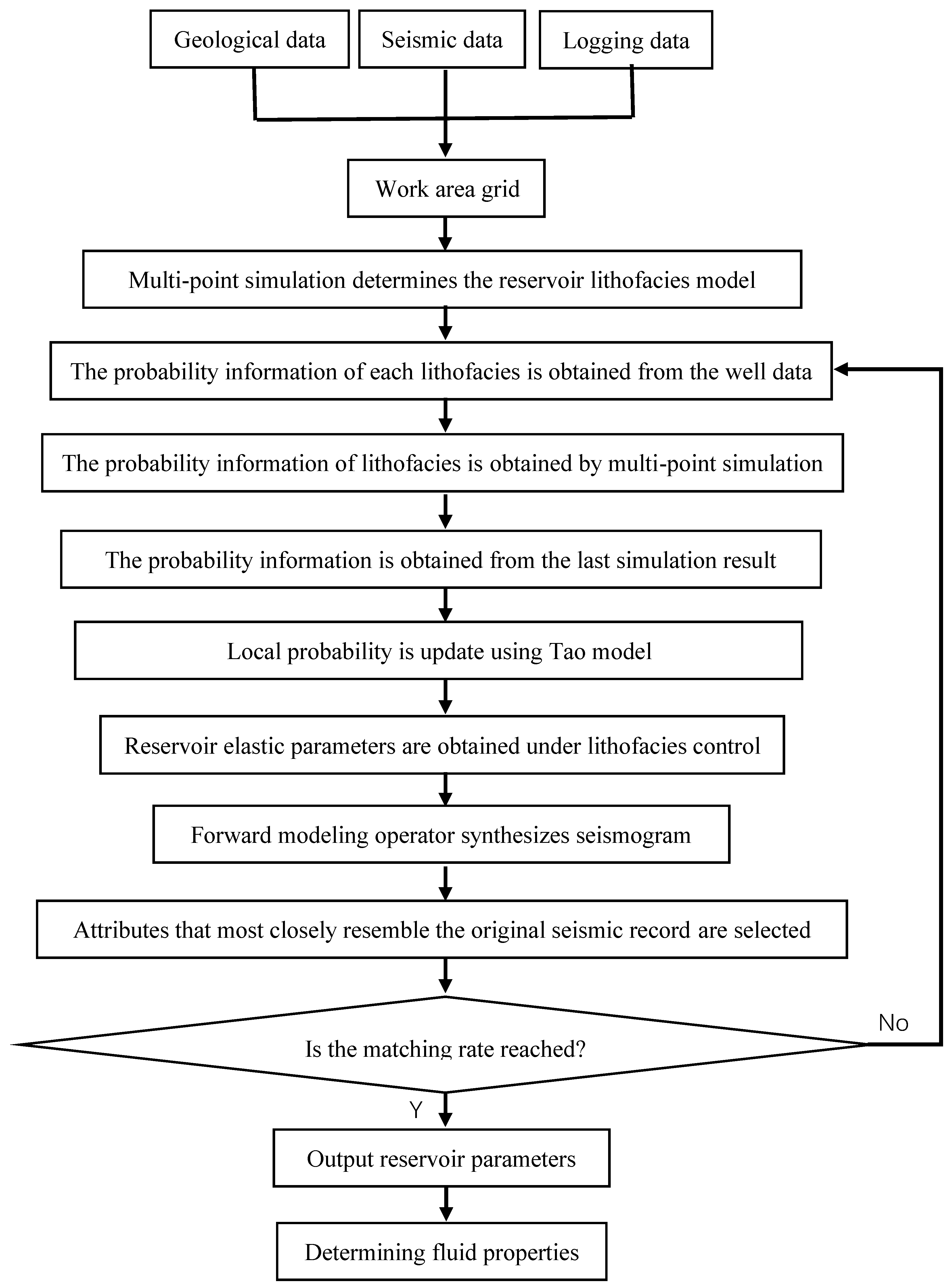
2.3. Inversion Steps

Based on the above improvements, a multi-point geostatistical inversion method based on the local probability updating method for the inversion of lithofacies (LPUMI) was developed in this study. The main steps are as follows (Figure 1).
Step 1: Preprocessing
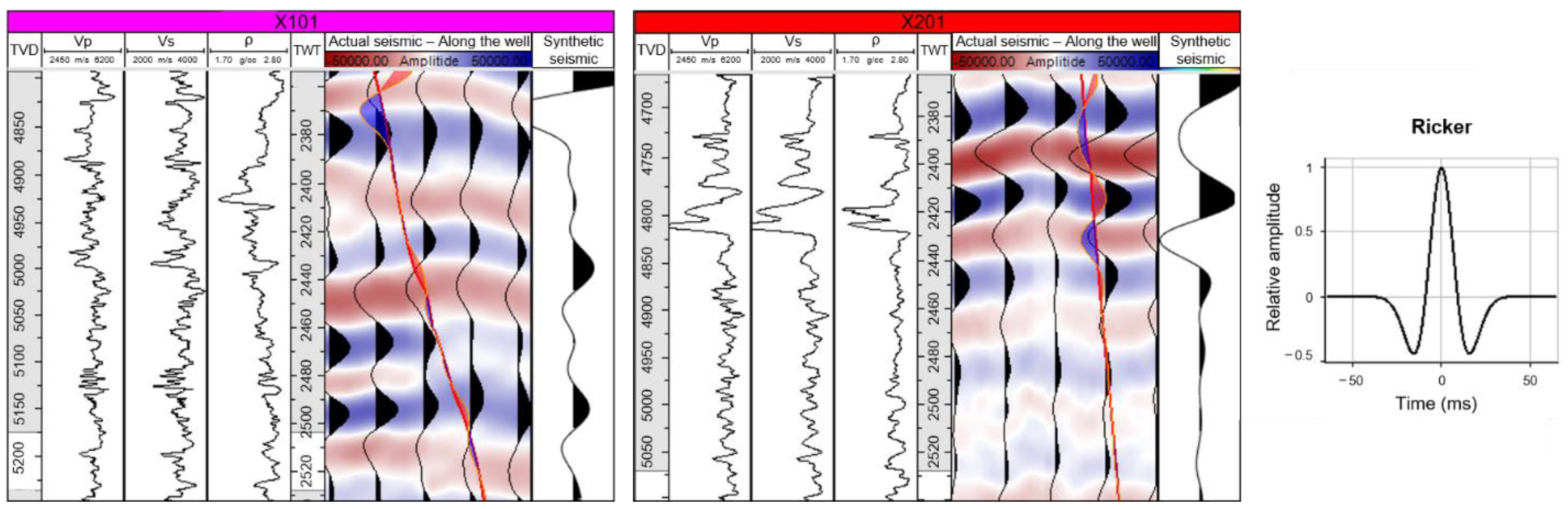
  • Check the data. Check whether the seismic data and well data are complete, including lithology, density, p-wave velocity, and s-wave velocity information.
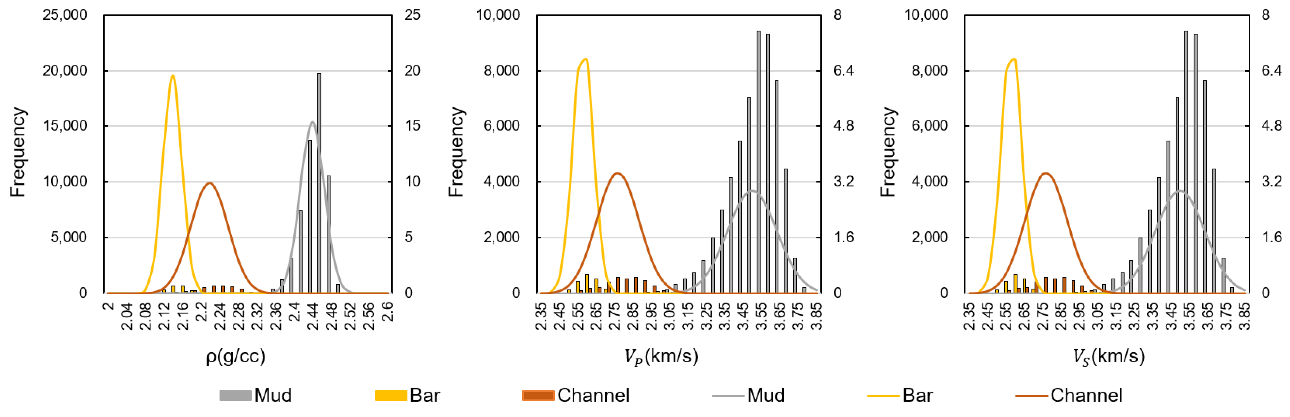
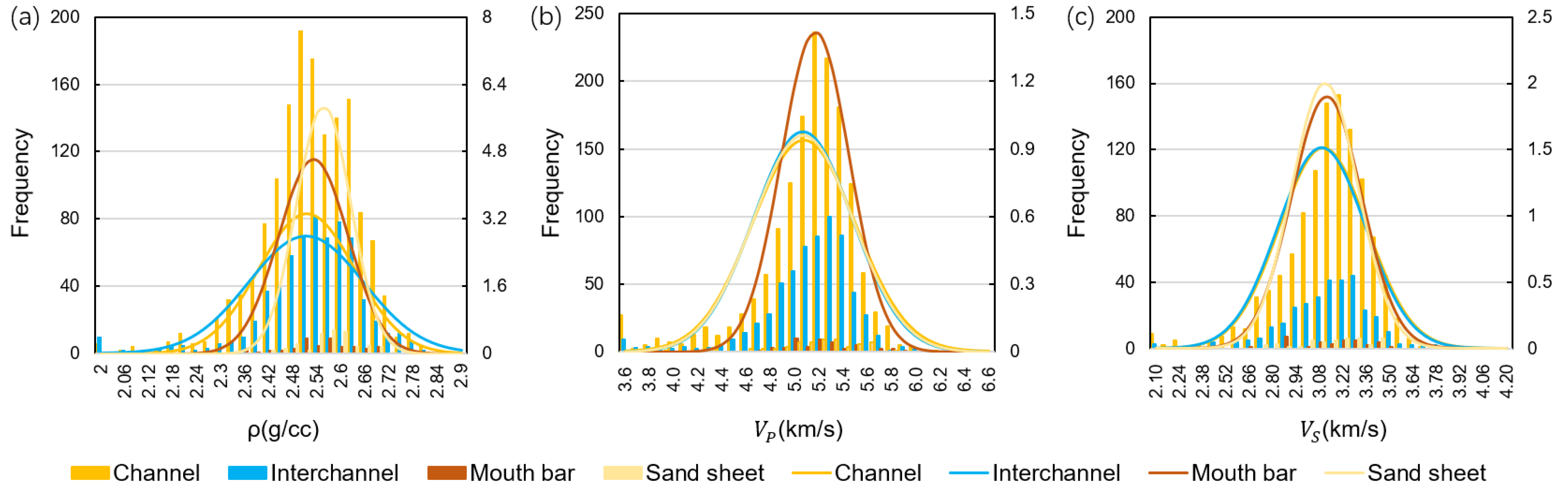
  • Statistical analysis of the data. When the shear wave information cannot be obtained from the logging data, it can be estimated using empirical formulas. The probability density functions of the different elastic parameters of the lithofacies are established to provide a basis for the subsequent elastic parameter sampling. The plot of the lithofacies versus the elastic parameters is established to provide a basis for the fluid prediction.
  • The attribute values of the initial reservoir elastic parameters are given. According to the statistical well data, the initial elastic parameter attribute values, including the density, p-wave velocity, and s-wave velocity, are assigned to the simulation grid.
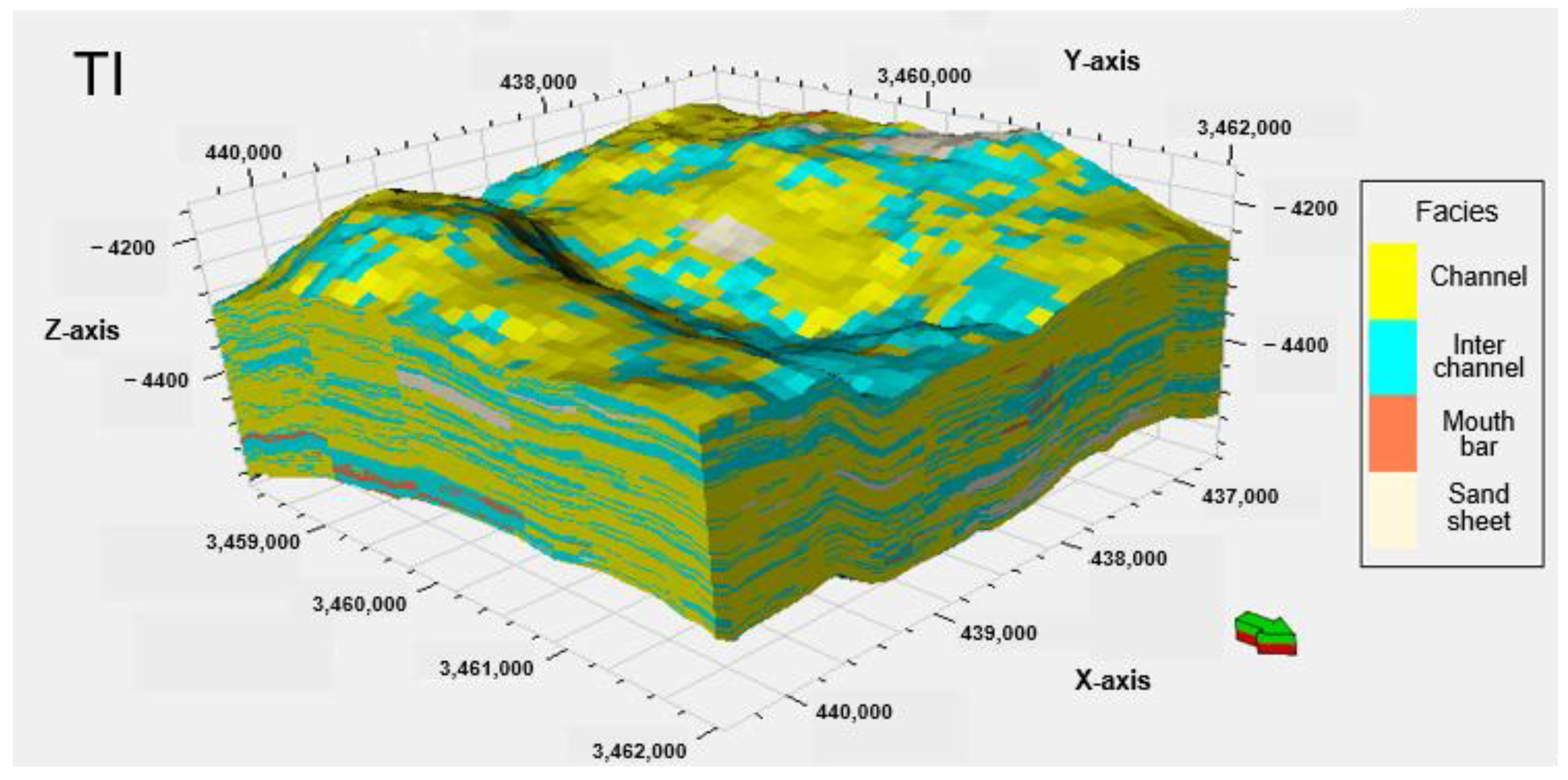
  • Build training images. Commonly, unconditional modeling methods such as object-based stochastic modeling, sedimentary process modeling, multi-point simulation results, outcrop and modern deposition models, digital geological sketches, and physical simulation interpretation are used to confirm the working area’s reservoir characteristics for the training images.
  • Scan the training images to establish a search tree. Only the data events that actually appear in the training image are saved in the search tree. In order to limit the geometric configuration of the data events and prevent it from being too large, the maximum number of searched data needs to be defined. Build a search tree based on the sample of the largest search data.
Step 2: SNESIM simulation using LPUMI
i.
Griding and assignment of the well data and elastic parameters. Each conditional data point is assigned to the nearest grid node in the simulation grid. If multiple conditional data points are assigned to the same grid node, the nearest one is assigned to the center of the grid node.
ii.
Define the path through the remaining nodes of the simulated grid. A path is a vector that contains all of the indexes of the grid nodes to be simulated in sequence. Random, one-way (i.e., the nodes are accessed in a regular order starting from one side of the grid), or any other path can be used. The simulation path is from a dense well area to a sparse well area and finally to a no well area.
iii.
Search for domains that simulate node X. They consist at most of n nodes {x1, x2, …, xN} that have recently been assigned to or simulated in the simulation grid. If the field of X is not found in the first iteration (such as the first unconditionally simulated node), a node Y is randomly selected in the TI, and its value (Z(y) to Z(x)) is assigned in the simulation grid. Then, proceed to the next node of the path.
iv.
Determine the search tree’s conditional probability P(A|B).
v.
Determine whether there is a point at which in the previous simulation, the elastic parameters were reserved. If there is, using the permanent ratio of the updating theory, probability P(A|B) will update to P(A|B,C). Otherwise, the update is still the conditional probability P(A|B).
Step 3: Prestack inversion
According to the reservoir’s elastic parameters obtained from the logging data, the density and p-wave velocity are uniformly sampled in the suggested data mode to obtain the p-wave impedance Z P of the sample.
According to the relationships between the p-wave impedance Z P and the s-wave impedance Z S and the p-wave impedance Z P and the density ρ given by Hampson and Russell (2005), in general, Z S and ρ can be expressed as follows:
ln Z S   = k ln Z P   +   k c + Δ L S ,
ln ρ   = m ln Z P   +   m c + Δ L D .
They are looking for deviations away from a linear fit in logarithmic space. k and m are the corresponding slop. k c and m c are the corrsponding intercept. The deviations away from this straight line, Δ L S and Δ L D , are desired fluild anomalies. The seismic forward modeling record calculation of the proposed elastic parameters in the proposed data model is conducted as follows:
g θ = c 1 ˜ W θ D L P + c 2 ˜ W θ D Δ L S + W θ D Δ L D ,  
where c 1 ˜ = 1 2 c 1 + 1 2 k c 2 + m c 3 ,   c 2 ˜ = 1 2 c 2 ,   c 1 = 1 + t a n 2 θ ,   c 2 = 8 γ 2 t a n 2 θ ,   c 3 = 0.5 t a n 2 θ + 2 γ 2 s i n 2 θ ,   γ = V S / V P .   W θ is the incident angle of the wavelet, D is the differential operator, L P = ln Z P , L S = ln Z S , L D = ln ρ , and g θ is the seismic forward modeling record.
The likelihood function Equation (3) and the posteriori probability Equation (4) are determined from the forward simulation record and the actual seismic record. Gonzalez’s (2008) method is adopted to select the elastic inversion parameters that retain the maximum likelihood function as the results; or according to the Metropolis–Hasting optimization criterion, a large number of implementations of the lithofacies and elastic parameters are generated from the posterior function, and these implementations represent the probability distribution of the posterior function. The acceptance criteria of the model are proposed to determine the optimal inversion elastic parameters.
P a c c e p t = m i n   ( 1 ,   P f * P f · exp m μ f 2 m * μ f 2 2 σ f 2 + d g m 2 d g m * 2 2 σ e 2 ) .
In consideration of the computational efficiency and algorithm continuity, Gonzalez’s [8] method was adopted in this study to select the optimal matching inversion results through iterative comparison of the multiple sampling (generally 25–30).
Step 4: Iteration
All of the simulation grids are visited to realize a single inversion.
According to the matching degree of the synthetic seismic records and the actual records, it is judged whether the iteration should be terminated. If the conditions are not met, start again from Step 2 for the next external iteration. Usually, after six iterations, the average correlation coefficient of the seismic data is greater than 85% and the inversion results are output.

3. Model Testing

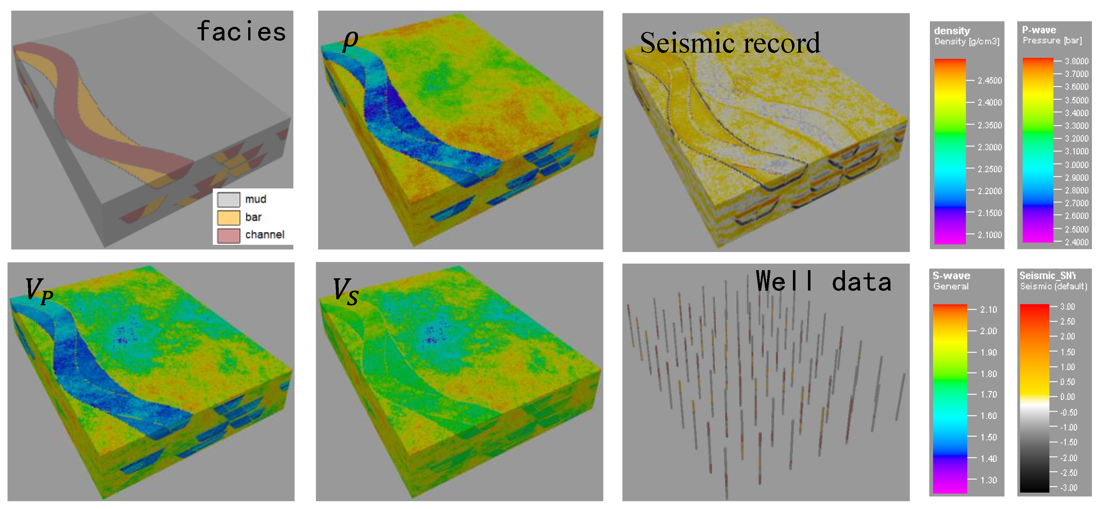
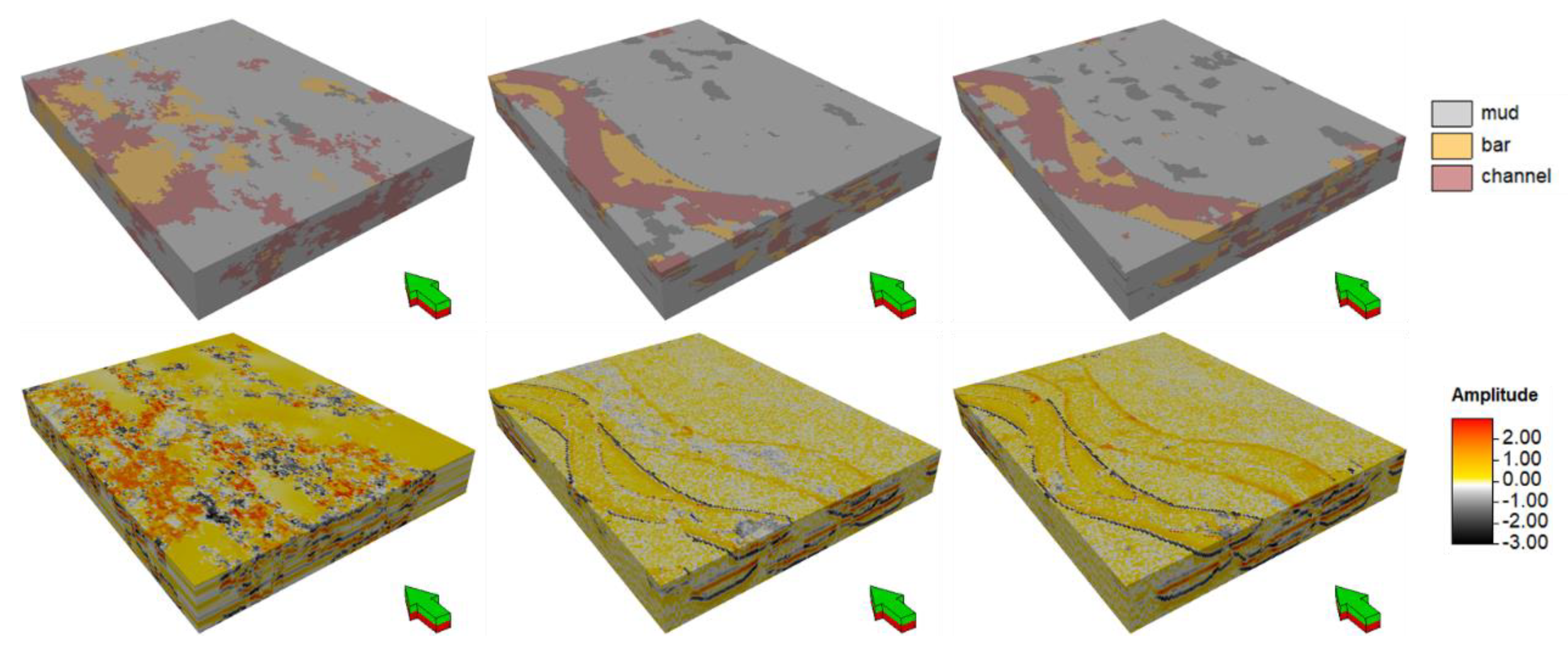
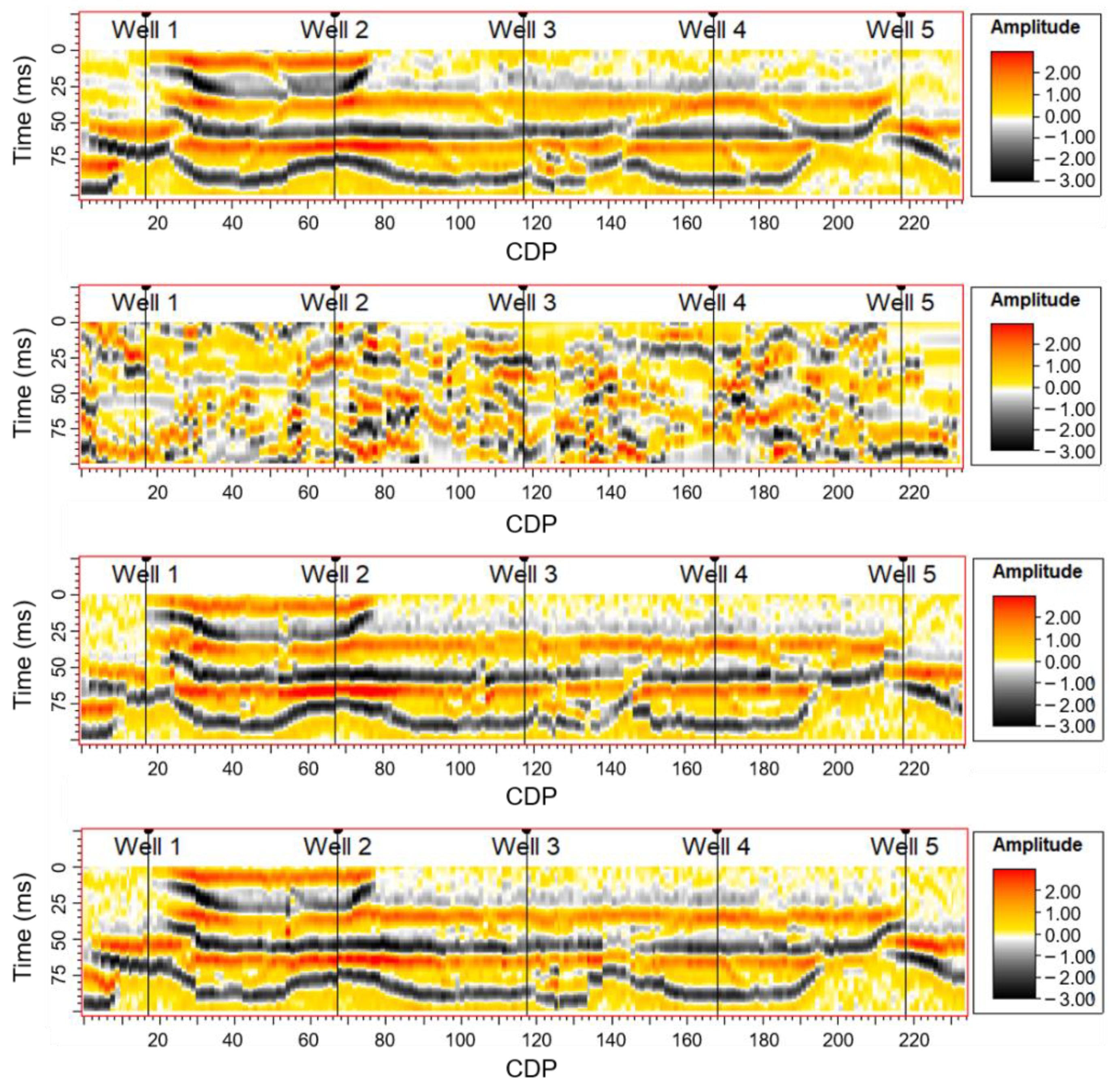
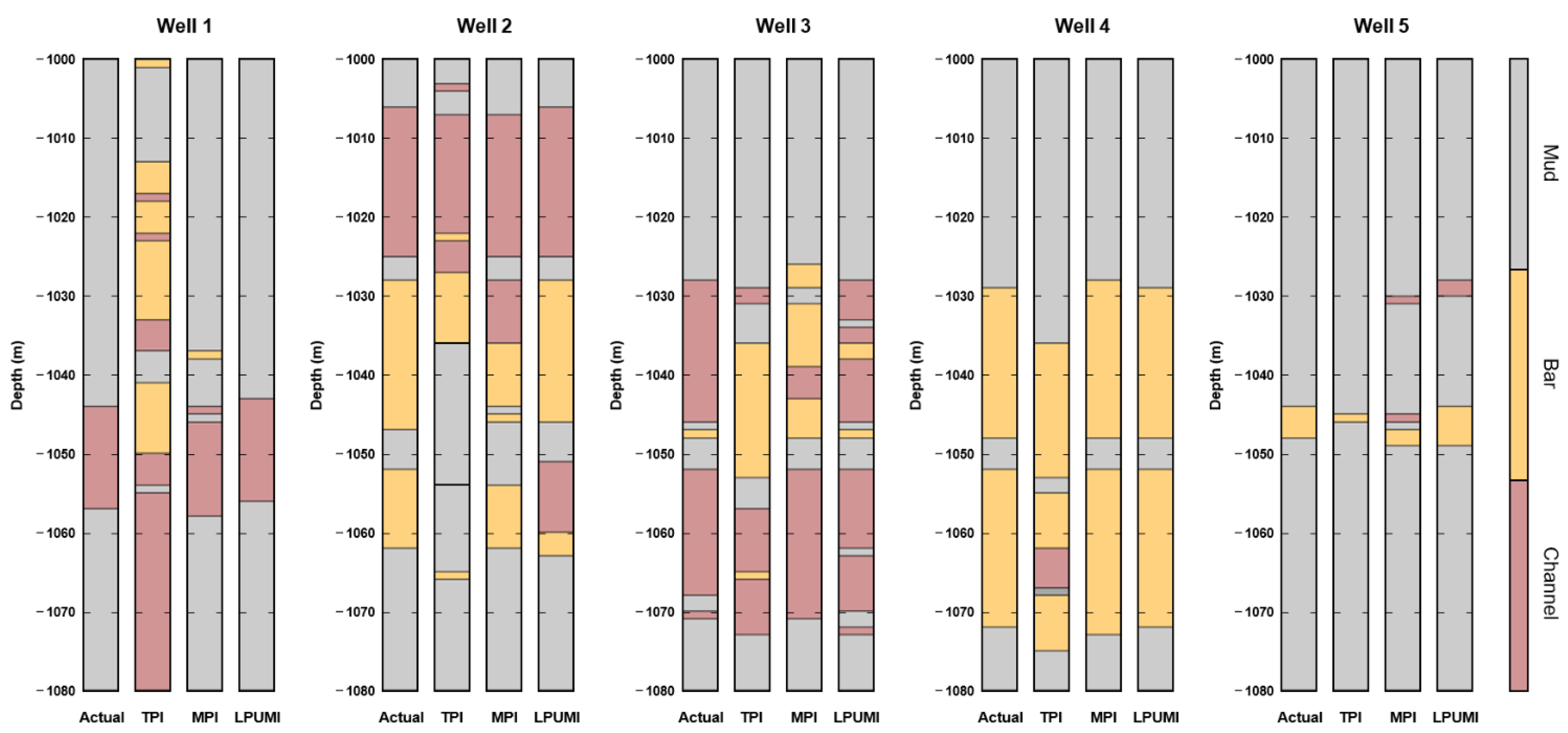
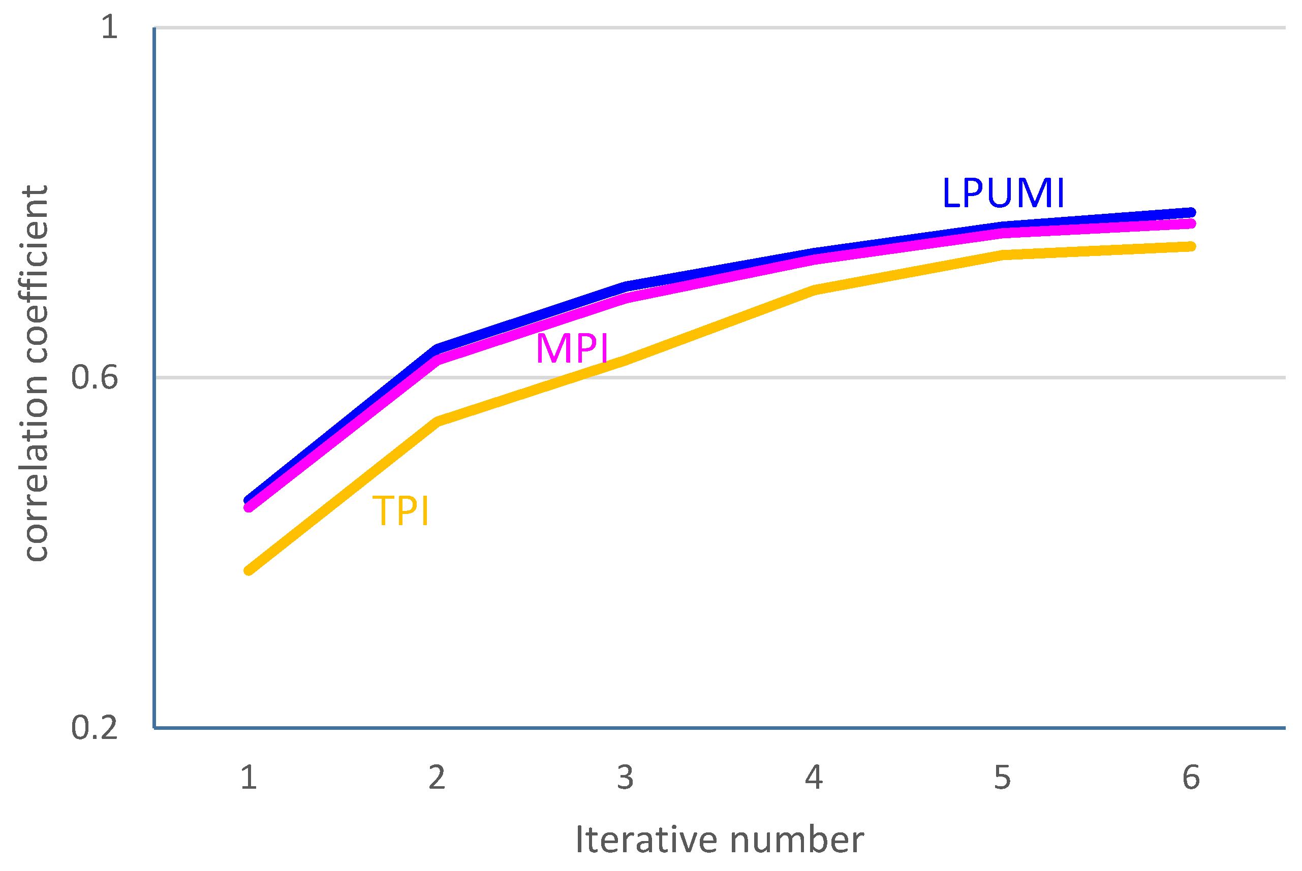
3.1. Theoretical Model Testing

The meandering river model with a low curvature in the first layer of the Stanford VI-E reservoir was taken as the test object, which is a 150 × 200 × 80 model. The lithofacies were subdivided into point bar, channel, and floodplain mudstone deposits (Figure 2). The different microfacies have different elastic parameter distributions (Figure 3). By designing 68 virtual wells, the seismic inversion method was tested based on the given elastic parameters and the lithofacies interpreted from the well data. In order to verify the accuracy of the method, only 63 wells were selected as the condition wells, and the remaining five wells were used as the test wells to analyze the inversion results.
The theoretical lithofacies model was selected as the training image, and the tests were carried out using the traditional two-point statistical inversion method (TPI), the conventional multi-point statistical inversion method (MPI), and the multi-point statistical inversion with local probability updating method (LPUMI). The results show that compared with two-point statistical inversion, multi-point statistical inversion can reproduce the reservoir lithofacies better, and the inversion results are more consistent with the theoretical model. The synthetic seismogram is more similar to the actual seismogram (Figure 4, Figure 5 and Figure 6). The average matching rate of the multi-point statistical inversion is 83.5%, while that of the two-point statistical inversion is 81.5%, indicating that the multi-point statistical inversion produced a more accurate prediction of the inter-well reservoir properties (Figure 7). According to the correlation coefficient of the seismic record calculated via the inversion, the correlation coefficient increases gradually as the number of iterations increases. After six iterations, the correlation between the inverted synthetic seismic track and the actual seismic track is close to 80%. The LPUMI has the largest correlation coefficient, reaching 0.78; the correlation coefficient of the MPI is in the middle (0.76); and the TPI has the lowest correlation coefficient (0.75) (Figure 8). The results show that the reservoir parameters obtained using the LPUMI are closer to the actual reservoir parameters. This shows that the proposed method is more reasonable and can be applied to actual reservoir inversion prediction.

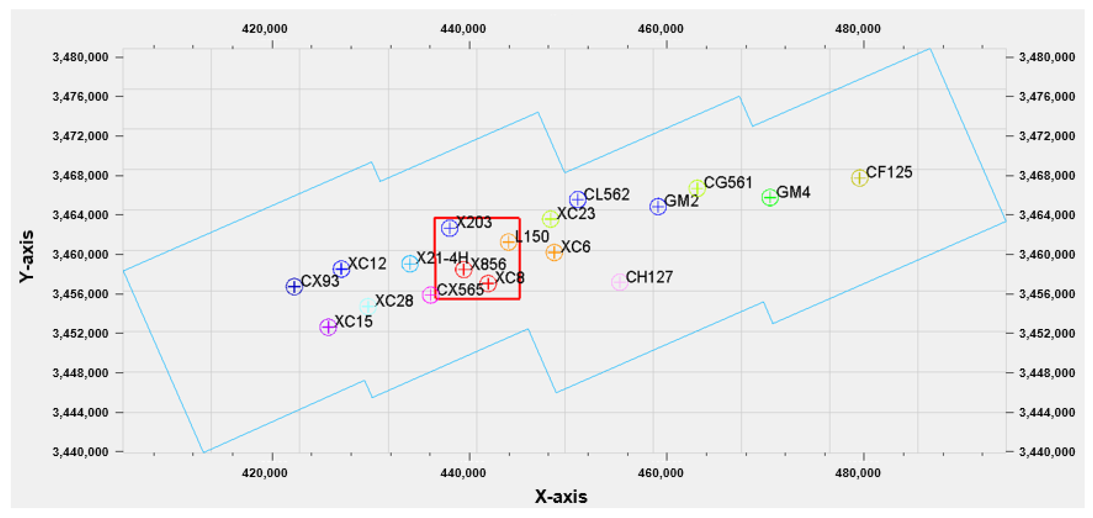
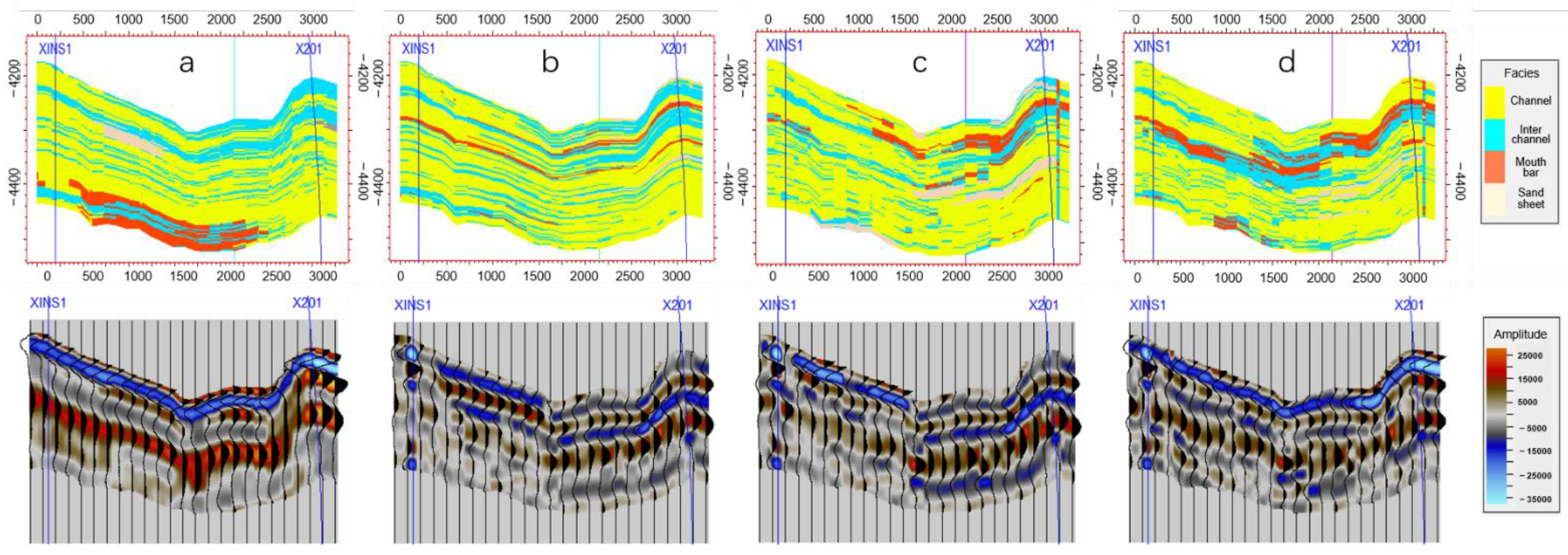
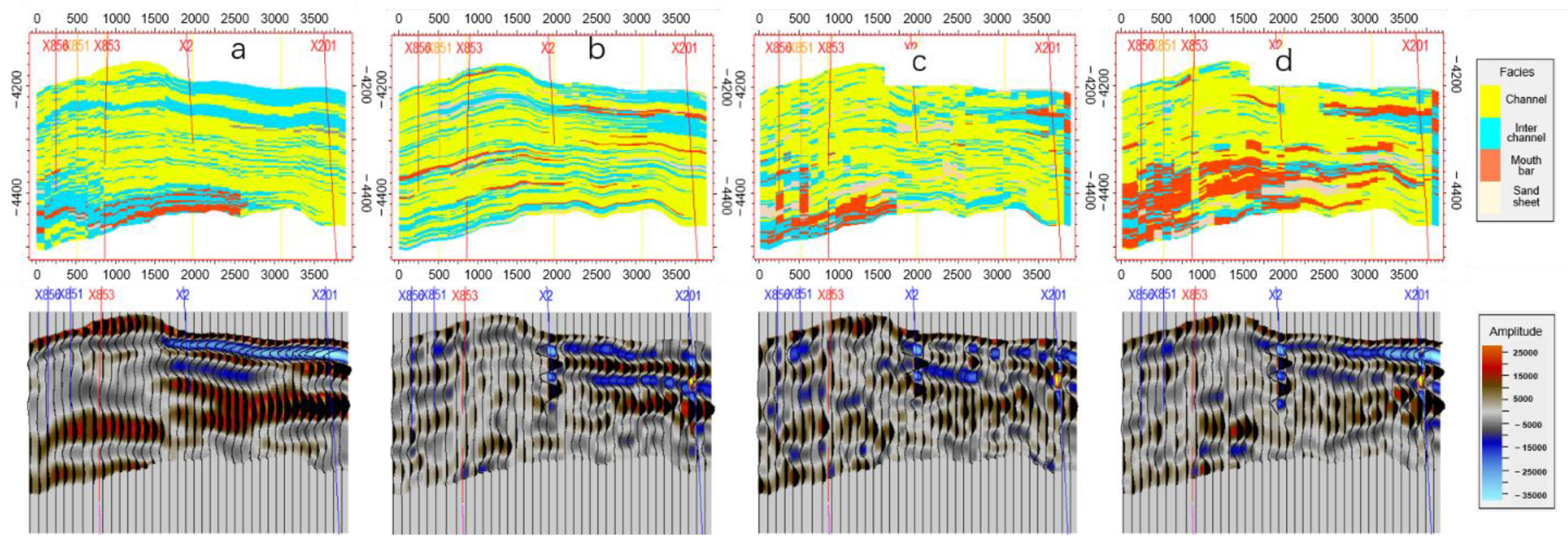
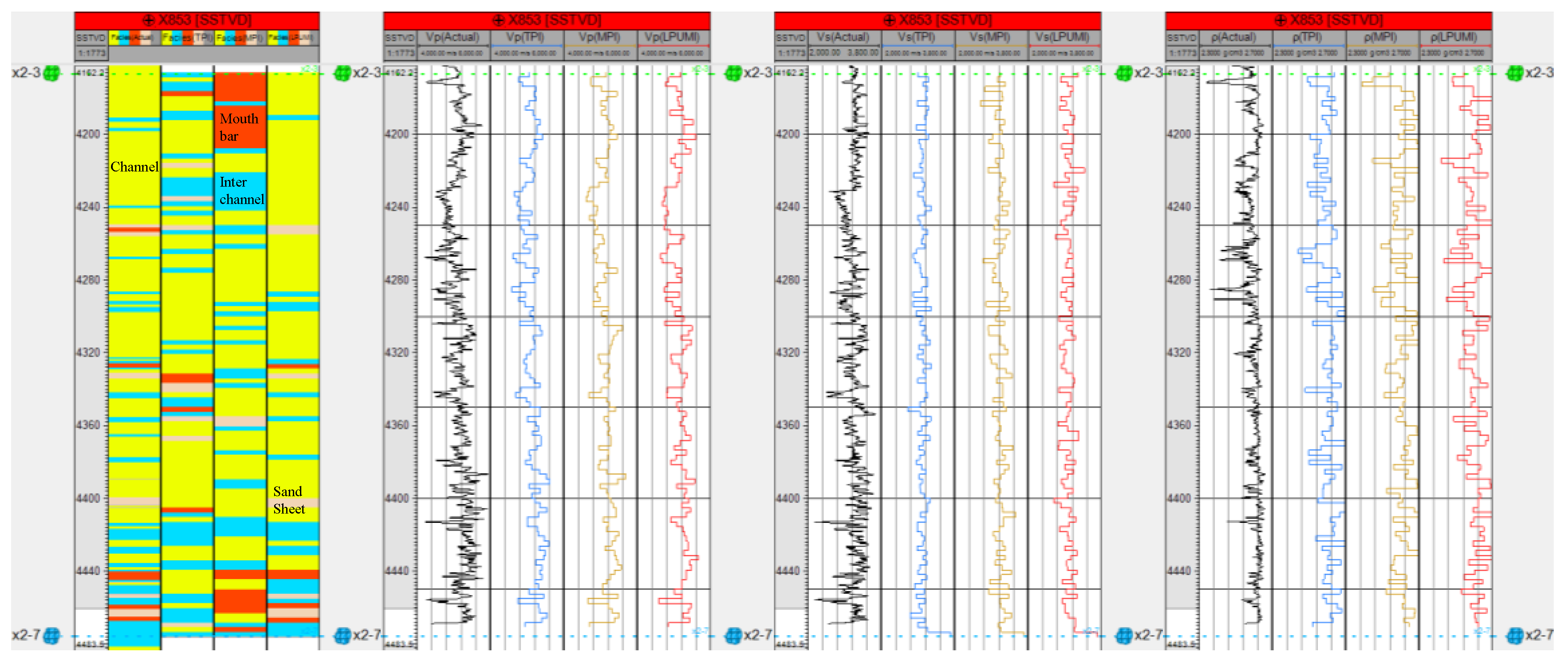
3.2. Real Reservoir Testing

The Xinchang gas field is located in the western part of the Sichuan Basin, China. The main gas-bearing horizon is the second member of the Xujiahe Formation, and the main sandbodies are braided delta front distributary channels and mouth bars. The thicknesses of the sand bodies are large and their horizontal distributions are wide. The horizontal distribution of the sweet spot reservoir is not uniform, which causes difficulties in the exploration and development of the gas reservoir.
In this study, three methods, including the TPI, MPI, and LPUMI, were applied to the prediction of the TX 2 3 TX 2 7 sand formation in the study area. Because this was mainly undertaken to test the proposed inversion method and compare it to the two existing methods, the inversion prediction was not performed for the entire region. Instead, a relatively regular local area with a relatively simple stratigraphic structure and no-fault development was selected to carry out the study. The total thickness of the vertical direction of the intercepted area is about 235 m, and the length in the I direction and J direction on the plane is about 4000 m (Figure 9). The grids were 100 × 100 m in the plane and 2 m in the vertical direction, and the total number of simulated grids was 40 × 40 × 118 = 188,800. Figure 10 shows the pre-stack track sets at different angles (5°, 15°, and 25°) in the test block. Figure 11 shows the spatial distribution and attribute interpretation for 11 wells. The analysis shows that the main body of the channel is composed of sand and silt, with little mud. The p-S wave velocity has an obvious linear relationship, with a small p-S wave velocity ratio and a low gamma ray (GR) value. The interchannel region is mainly composed of clay deposits with a small amount of silt and fine sand. The p-S wave velocity has an obvious linear relationship, with a high p-S wave velocity ratio and a high GR value. The mouth bar is composed of fine and silty sand, with fine sorting and a pure quality, and it has a small S-wave velocity ratio and low GR value, which is similar to the main body of the channel (Figure 12). The statistical analysis of the elastic parameter–lithofacies was conducted based on the data for these 11 wells, and its probability distribution was established for the elastic parameter sampling under lithofacies control during the subsequent inversion (Figure 13). The seismic wavelets from different angles were extracted based on the seismic records of the sidewalks (Figure 14). After comprehensive analysis, 25 Hz theoretical Rick wavelets were selected for the inversion seismic record synthesis. Based on geological analysis, a three-dimension training image of the study area was established (Figure 15), which was used to calculate the two-point variogram function and to extract the multi-point prior probability.
The inversion profile results obtained using the different method were captured for wells Xins1–X201 for comparison (Figure 16). As can be seen from the profiles, overall, all of the inversion lithofacies profiles are mainly composed of channel sand bodies. The mouth bar deposits are locally developed, and the mudstone deposits are relatively scarce and are mainly developed in the upper part. The lithofacies inversion is relatively continuous and the distribution of the channel sand body is reflected well. However, in terms of the structure, the sand body continuity of the TPI is too good to reflect the complex heterogeneity. The distributions of the MPI and LPUMI are highly variable and are connected locally, and the overall structure is close to that of the actual reservoir. In terms of the seismic track records, the inversion seismic records of the MPI and LPUMI are close to the actual seismic records, while the TPI exhibits chaotic reflection characteristics, which are quite different from the actual continuous lithofacies distribution. The results show that the MPI and LPUMI are able to reflect the sand body and elastic parameters better.
Gonzalez [8] pointed out that the accuracies of the inversion iterations can be compared using the absolute error recorded by the forward simulation or the seismic trace correlation. Due to the possible errors in the time–depth conversion, direct comparison may cause large errors. However, the underground reservoir prediction is more likely to reveal the sand body and the spatial structure of the interlayer. If the reflected structure is similar, the overall similarity of the seismic records will increase. Therefore, the correlation between the forward simulation records and the actual records was used to compare the results of the different methods. The correlations between the forward modeling records and the actual seismic track were calculated. The results show that the correlation coefficient of the TPI is 0.72. The correlation coefficient of the MPI is 0.74, and that of the LPUMI is 0.77. This demonstrates that the LPUMI results are closer to the actual seismic record and have a higher accuracy.
Furthermore, the cross-validation method was used to test and compare the methods. The cross section of well X853 was used to compare the prediction accuracies of the different methods. Both the MPI and LPUMI can reflect the characteristics of the upward transition of the mouth bar sand body, which is consistent with the migration trend of the lithofacies in the training image. However, the TPI can hardly reflect this characteristic. Compared with the actual seismic record, the synthetic seismic records of the MPI and LPUMI are closer to the actual seismic profile (Figure 17).
According to the comparison of the elastic parameters across well X853 (Figure 18), the different inversion methods can reflect the variations in the elastic parameters in the area around the well successfully, with a good degree of matching. In terms of the elastic parameter errors, the TPI performed the best, followed by the MPI and the LPUMI. However, the differences are not significant. In terms of the correlation of the elastic parameters, the overall difference is not significant. The correlation of the LPUMI is 0.74, that of the MPI is 0.73, and that of the TPI is 0.72. However, the degrees of lithofacies matching are different. The results show that the best method is the LPUMI (0.862), followed by the MPI (0.856), and the TPI is the worst (only 0.78). This indicates that the LPUMI has more advantages.

4. Discussion

Seismic records are a comprehensive representation of subsurface lithofacies, physical properties, elastic parameters, and fluids. The essence of statistical inversion is to seek the optimal solution that reflects the underground reservoir parameters through convolution of the elastic parameters. The distribution of the elastic parameters is mainly revealed through rock physics modeling. In the field of geological modeling, due to the intrinsic relationship between the lithofacies and physical properties, developing facies-controlled reservoir parameter modeling method has become an important means of improving the accuracy of physical property modeling. Therefore, introducing the idea of facies control into seismic inversion can improve the inversion accuracy. In fact, Azevedo and Soares [29] compared the inversion results of the given lithofacies model with conventional inversion results and showed that the inversion elastic parameter distribution of the given lithofacies model is more reasonable and the iteration convergence is faster. Based on the theoretical model and practical model developed and tested in this study, the multi-point inversion method considering facies control is significantly better than the traditional two-point statistical inversion method without facies control. Therefore, making full use of lithofacies control in seismic inversion should be an important direction in the future. In a sense, the accuracy of the constrained lithofacies model determines the effectiveness of the final inversion effect.
In this improvement, the seismic elastic parameters are mainly used for local lithofacies updating. The SNESIM method is a single-grid point lithofacies forecasting method. When using elastic parameters to update the local lithofacies, only the information provided by the elastic parameters of the points to be estimated is used, which has no significant improvement effect compared with the conventional multi-point geostatistical inversion. This may be due to the fact that grid by grid updating of lithofacies does not significantly change the sedimentary facies model. In addition, probabilistic statistical sampling errors inevitably exist and are transmitted to the subsequent updates, resulting in limited improvement of the inversion accuracy. Another disadvantage of the SNESIM lithofacies prediction is that all reservoir predictions based on statistical methods require a stable lithofacies distribution model, but in reality, the lithofacies distribution is very complex and has non-stationary characteristics. This is one of the reasons why multi-point statistical methods such as the SIMPAT, Filtersim, and DS methods have been developed. This is also the reason why Gonzalez [8] used SIMPAT as the lithofacies inversion method.
Arpat (2005) pointed out that seismic information can be integrated in SIMPAT geological modeling; that is, a seismic reference image with a good correspondence to the lithofacies can be constructed, and its contribution to the distance can be taken into account in the lithofacies matching to constrain and guide the selection of the optimal lithofacies mode:
s , = s h d e v T ( u ) , p a t T k + s s s d e v T ( u ) , s p a t T k ,  
where s h d e v T ( u ) , p a t T k is the similarity between the model at the point to be estimated d e v T ( u ) and the data model p a t T k in the lithofacies training image s s s d e v T ( u ) , s p a t T k and the similarity between the seismic attribute model s d e v T ( u ) at the corresponding point to be estimated and the seismic attribute model s p a t T k in the training image. It should be noted that the contribution of the seismic attributes (i.e., soft data) is different from that of well data (i.e., hard data), so it is necessary to effectively measure the contribution of the seismic attributes. The similarity value of the seismic training images is multiplied by a weight to represent the contribution of the seismic attributes in the similarity calculation. In addition, because the scale of the seismic attributes is not consistent with that of the facies attributes, the seismic attributes must be normalized before the similarity calculation in the application of the seismic data in order to avoid the absolute superiority of the seismic similarity in the entire similarity due to the different scales.
Lithofacies training images can be obtained from the geological anatomy and through sedimentary simulation. However, seismic attribute training image is often difficult to obtain. Based on rock physics modeling, the forward modelling can be conducted many times and the optimal matching seismic attributes can be calculated, which can be applied to Equation (15) to update the overall local lithofacies and improve the accuracy of the inversion.
The efficiency of the mSIMPAT algorithm is relatively low, and adding seismic attribute constraints will further increase the computational burden. Therefore, using parallel computing and deep learning theory to accelerate the inversion iteration is an important direction in future research.

5. Conclusions

This paper proposed a new multi-point geostatistical inversion through local iterative updating rock facies using the constrains of elastic parameters. An internal and external double cycle iteration mechanism was adopted to execute the iteration and updating. During the internal cycle iteration, the optimal elastic parameters obtained in the previous external cycle were combined with the statistical probability of the lithofacies and elastic parameters, and the elastic parameters were combined with the permanent ratio of the updating theory to achieve local lithofacies updating. Based on this, inversion prediction of the lithofacies and elastic parameters was carried out. In the outer loop, the current global inversion results were compared with the actual error to determine whether the inversion results of the elastic parameters meet the conditions, and the cycle iteration was carried out again until local elastic parameter inversion and global inversion satisfy the given conditions. Then, the cycle was terminated and the inversion results were output.
Both the theoretical and practical model tests conducted confirm that the correlation between the actual seismic track and the synthetic seismic track obtained using the LPMUI is the best, and the degree of lithofacies matching is the highest. The results of the MPI are the next best, and the results of the TPI are the worst, indicating that the reservoir parameters obtained using the LPMUI are closer to the actual reservoir parameters. This method is worth popularizing in practical exploration and development.
The calculation efficiency of double iteration in the LPMUI is much better than traditional MPI; however, it is still lower than the TPI. In future, the deep learning method or parallel computing method can be introduced to improve the calculation efficiency. Another improvement may exist in the use of the elastic parameters for rock lithofacies updating. Here, only the elastic property in the un-simulated grid was used to update the rock lithofacies in the same grid, a multi-point geostatistical simulation for sedimentary pattern reproduction and updating was not conducted, which may have caused the failure of the reproduction of a continuous geobody. How to use elastic parameters in a multi-point data template to update rock lithofacies patterns, is still a challenge for future work.

Author Contributions

Conceptualization, Y.Y. and T.C.; methodology, X.H. and L.W.; software, X.H.; validation, Z.W.; formal analysis, Z.W.; investigation, Z.W.; resources, T.C.; data curation, Z.W.; writing—original draft preparation, Z.W.; writing—review and editing, Z.W., X.H. and Y.Y.; visualization, X.H.; supervision, Z.W. and Y.Y.; project administration, Y.Y.; funding acquisition, Y.Y. All authors have read and agreed to the published version of the manuscript.

Funding

This work is supported by the National Natural Science Foundation of China (Grant Numbers 42130813 and 41872138).

Conflicts of Interest

The authors declare no conflict of interest.

Abbreviations

The following abbreviations are used in this manuscript:
LPUMIa multi-point geostatistical inversion method based on the local probability updating method for the inversion of lithofacies.
MCMCMarkov chain Monte Carlo.
ASRadaptive spatial resampling.

References

  1. Ghaderpour, E. Multichannel antileakage least-squares spectral analysis for seismic data regularization beyond aliasing. Acta Geophys. 2019, 67, 1349–1363. [Google Scholar] [CrossRef]
  2. Bosch, M.; Mukerji, T.; Gonzalez, E.F. Seismic inversion for reservoir properties combining statistical rock physics and geostatistics: A review. Geophysics 2010, 75, 165–176. [Google Scholar] [CrossRef] [Green Version]
  3. Zhang, F.; Xiao, Z.; Yin, X. Bayesian stochastic inversion with seismic data constraints. Oil Geophys. Prospect. 2014, 49, 176–182. [Google Scholar]
  4. Journel, A.G.; Huijbregts, C.J. Mining Geostatistics; Academic Press: New York, NY, USA, 1978. [Google Scholar]
  5. Haas, A.; Dubrule, O. Geostatistical inversion-a sequential method of stochastic reservoir modelling constrained by seismic data. First Break. 1994, 12, 561–569. [Google Scholar] [CrossRef]
  6. Deutsch, C.V. GSLIB Geostatistical Software Library and User’S Guide; Oxford University Press: Oxford, UK, 1992. [Google Scholar]
  7. Bortoli, L.J.; Alabert, F.A.; Hass, A.; Journel, A.G. Constraining Stochastic Images to Seismic Data; Geostatistics Tróia’92. Spring: Dordrecht, The Netherlands, 1993; pp. 325–337. Available online: https://www.semanticscholar.org/paper/Constraining-Stochastic-Images-to-Seismic-Data-Bortoli-Alabert/20d8acea057bcc1d7f875a204689c2ee1243ad73 (accessed on 21 December 2021).
  8. González, E.F.; Mukerji, T.; Mavko, G. Seismic inversion combining rock physics and multiple-point geostatistics. Geophysics 2008, 73, 11–21. [Google Scholar] [CrossRef]
  9. Yang, P.J.; Yin, X.Y. Non-linear quadratic programming Bayesian prestack inversion. Chin. J. Geophys. 2008, 51, 1876–1882. (In Chinese) [Google Scholar]
  10. Zhang, G.; Wang, D.; Yin, X. Seismic parameters estimation using MCMC method. Oil Geophys. Prospect. 2011, 46, 605–609. [Google Scholar]
  11. Wang, P.; Li, Y.; Zhao, R. Lithology inversion using post-stack MCMC method. Prog. Geophys. 2015, 30, 1918–1925. [Google Scholar]
  12. Azevedo, L.; Demyanov, V. Multi-scale uncertainty assessment in geostatistical seismic inversion. Geophysics 2019, 84, R355–R369. [Google Scholar] [CrossRef]
  13. Pereira, P.; Calçôa, I.; Azevedo, L.; Nunes, R.; Soares, A. Iterative geostatistical seismic inversion incorporating local anisotropies. Comput. Geosci. 2020, 24, 1589–1604. [Google Scholar] [CrossRef]
  14. Caers, J.; Srinivasan, S.; Journel, A.G. Geostatistical quantification of geological information for a Fluvial-Type North Sea Reservoir. In Proceedings of the SPE Annual Technical Conference and Exhibition, SPE-56655-MS. Houston, TX, USA, 3–6 October 1999. [Google Scholar]
  15. Strebelle, S.; Journel, A.G. Reservoir modeling using multiple-point statistics. In Proceedings of the SPE Annual Technical Conference and Exhibition, SPE-71324-MS. New Orleans, LA, USA, 30 September–3 October 2001. [Google Scholar]
  16. Yin, Y.; Zhang, C.; Li, J.; Shi, S. Research progress and Prospect of multi-point geostatistics. J. Palaeogeogr. 2011, 13, 245–253. [Google Scholar]
  17. Yang, P. Geostatistical inversion: From two points to multiple points. Prog. Geophys. 2014, 29, 2293–2300. [Google Scholar]
  18. Yang, P. Multi-point geostatistical random simulation based on pattern clustering and matching. Prog. Geophys. 2018, 33, 279–284. [Google Scholar]
  19. Guardiano, F.B.; Srivastava, R.M. Multivariate Geostatistics: Beyond Bivariate Moments. In Geostatistics Tróia ’92, Quantitative Geology and Geostatistic; Kluwer Academic Publications: Dordrecht, The Netherlands, 1993; pp. 133–144. [Google Scholar]
  20. Jeong, C.; Mukerji, T.; Mariethoz, G. A fast approximation for seismic inverse modeling: Adaptive spatial resampling. Math. Geosci. 2017, 49, 845–869. [Google Scholar] [CrossRef]
  21. Liu, X.; Li, J.; Chen, X.; Li, C.; Guo, K.; Zhou, L. A stochastic inversion method integrating multi-point geostatistics and sequential Gaussian simulation. Chin. J. Geophys. 2018, 61, 2998–3007. [Google Scholar]
  22. Liming, S.; Wuyang, Y.; Fengchang, Y.; Xingyao, Y.; Xueshan, Y. Review and prospect of seismic inversion technology. Oil Geophys. Prospect. 2015, 50, 184–202. [Google Scholar]
  23. Ling, Y.; Xiao, Y.; Sun, D.; Lin, J.; Gao, J. Influence factors analysis and seismic attribute interpretation of post-stack thin reservoir inversion. Geophys. Prospect. Pet. 2008, 47, 531–558. [Google Scholar]
  24. Azevedo, L.; Nunes, R.; Soares, A.; Mundin, E.C.; Neto, G.S. Integration of well data into geostatistical seismic amplitude variation with angle inversion for facies estimation. Geophysics 2015, 80, 113–128. [Google Scholar] [CrossRef]
  25. Azevedo, L.; Soares, A. Geostatistical Methods for Reservoir Geophysics; Springer International Publishing: Cham, Switzerland, 2017. [Google Scholar]
  26. Tarantola, A. Inverse Problem Theory and Methods for Model Parameter Estimation; Society for Industrial and Applied Mathematics: Philadelphia, PA, USA, 2005; pp. 269–285. [Google Scholar]
  27. Mariethoz, G.; Renard, P.; Straubhaar, J. The direct sampling method to perform multiple-point geostatistical simulations. Water Resour. Res. 2010, 46, 1–14. [Google Scholar] [CrossRef] [Green Version]
  28. Journel, A.G. Combining knowledge from diverse sources: An alternative to traditional data independence hypotheses. Math. Geol. 2002, 34, 573–596. [Google Scholar] [CrossRef]
  29. Arpat, B.G. Sequential Simulation with Patterns. Doctoral Dissertation, Stanford University, Stanford, CA, USA, 2005. [Google Scholar]
Figure 1. New multi-point geostatistical inversion flow chart considering local updating.
Energies 15 00299 g001
Figure 2. Stanford VI-E theoretical model.
Energies 15 00299 g002
Figure 3. Statistical distribution of the elastic parameters of the different microfacies.
Energies 15 00299 g003
Figure 4. Lithofacies and forward modeling records of the inversion (left) TPI, (middle) MPI, and (right) LPUMI.
Energies 15 00299 g004
Figure 5. Lithofacies profiles of the five validation wells (from top to bottom, real reservoir, TPI, MPI, and LPUMI).
Energies 15 00299 g005
Figure 6. Seismic records obtained through well inversion (from top to bottom, real reservoir, TPI, MPI, and LPUMI).
Energies 15 00299 g006
Figure 7. Comparison of the lithofacies distribution in five wells obtained using the different methods.
Energies 15 00299 g007
Figure 8. Correlation coefficients between the inversion trace and actual trace.
Energies 15 00299 g008
Figure 9. Drilling distribution map of the actual working area and the location of the inversion block.
Energies 15 00299 g009
Figure 10. Pre-stack seismic track set for the inversion block: (a) 5°, (b) 15° and (c) 25°.
Energies 15 00299 g010
Figure 11. Data interpretation results for the 11 wells in the inversion block: (a) lithofacies, (b) density, (c) p-wave velocity, and (d) s-wave velocity.
Energies 15 00299 g011
Figure 12. Statistical diagram showing the relationship between the elastic parameters and the lithofacies.
Energies 15 00299 g012
Figure 13. Analysis of the elastic parameters of the different lithofacies in the wells: (a) density, (b) p-wave velocity, and (c) shear wave velocity.
Energies 15 00299 g013
Figure 14. The synthetic and observed seismic traces.
Energies 15 00299 g014
Figure 15. Training image of the inversion block.
Energies 15 00299 g015
Figure 16. Inversion of the lithofacies model and synthetic seismic record through wells xins1–X201 for the training image and the different methods: (a) Training image, (b) TPI model, (c) MPI model, and (d) LPUMI model.
Energies 15 00299 g016
Figure 17. Training image and lithofacies model inversions obtained using the different methods and forward simulation records of well X853 through the drainage: (a) Training image, (b) TPI lithofacies model, (c) MPI lithofacies model, and (d) LPUMI lithofacies model.
Energies 15 00299 g017
Figure 18. Comparison between the predicted results and the actual lithofacies and elastic parameters of the well.
Energies 15 00299 g018
Publisher’s Note: MDPI stays neutral with regard to jurisdictional claims in published maps and institutional affiliations.

