Abstract
A fundamental task in the dynamic simulation of parabolic trough power plants (PTPP) is to understand the behavior of the system physics and control loops in the presence of weather variations. This study provides a detailed description of the advanced controllers used in the power block (PB) of a 50 MWel parabolic trough power plant (PTPP). The PB model is achieved using APROS software based on the actual specifications of the existing power plant. To verify the behaviour of the PB model, a comparison between the simulated results and given real data is documented depending on a previous study, and the results indicate a reasonable degree of correspondence. The purpose of this study is to create reference models for the PB. Thereby, developers and engineers will have a better understanding of the state of the art of advanced control loops in these power plants. Moreover, these types of models can be used to specify the most suitable mode of operation for the power plant. In addition, this study gives an overview of dynamic simulation for the design, optimisation and development of power blocks in parabolic trough power plants.
1. Introduction
Fossil resource limitations and serious environmental challenges need to create new renewable power generation alternatives that are now economically viable [1]. Nowadays, there are four main types of concentrating solar power technologies, namely parabolic trough (PT), linear Fresnel reflector (LFR), central tower (CT) and parabolic dish technology (PD) [2]. Concentrating solar power (CSP) has proven to be a renewable energy technology, and in the future it will be cost-efficient, as it generates electrical power from solar irradiation [3]. Different operating fluids such as thermal oil, water and molten salt are used in these technologies [4]. Among the CSP technologies, parabolic trough technology is the most mature of the concentrating solar power plants, and it is commercially proven [5]. The parabolic trough solar power plant can be classified as one of the best solar energy technologies used to produce electrical energy [6]. The solar radiation is focused using mirrors on the solar energy receivers, where it is then converted to electricity or heat [7]. Generally, parabolic trough power plants include three main parts, namely solar field (SF), thermal storage system (TSS) and power block (PB) [8,9], as shown in Figure 1. Furthermore, a fossil fuel unit can be included in these power plants for improving the plant’s potential [10].
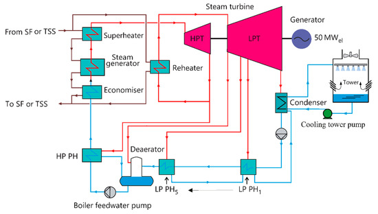
Figure 1.
Parabolic through power plant with thermal storage system.
Dynamic simulation provides an efficient approach for improving the efficiency of PTPP and for evaluating the capability and specifications of the plant regarding materials, process, emissions, or economics [11].
Two different types of models can be found in the literature, which either simulate the parabolic trough power plants depending on constant time steps, and deal with most power plant components as quasi-static simulation [9] or follow the periods of few clouds and transient periods using a basic approach [12]. The most important inputs to the dynamic models are direct normal irradiance (DNI), wind speed, humidity and ambient temperature [13].
Several commercial programmes are used in the parabolic trough power plant modelling, namely EBSILON Professional [14], IPSEpro [15], EcoSimPro [16], GATECYCLE [17], TRNSYS [18], DYMOLA [19], ASPEN [20], MATHEMATICA [21], SOLERGY [22] as well as System Advisor Model (SAM) [23]. Recent works have also used the APROS software for the modelling and simulation of PTPP, as proven in [24,25]. It should be mentioned here that what distinguishes the APROS program is the high dynamic and fast response to fluctuations that occur during long and short periods of operation, unlike the rest of the programs used. Moreover, APROS contains statistical data for different latitude and longitude, in addition to the different days of the year. A compressive overview of programmes applicable to concentrating solar power technologies was presented in [26]. As this solar technology is most widely used, it provides a more realistic operational data, and for this reason, it is used to validate the dynamic models [27].
The dynamic simulation models are used to understand the behavior of the PTPP during weather changes. It is obvious that few dynamic simulation models regarding parabolic trough technology have been implemented so far. However, most of these studies conducted the storage system and solar field models, while very few studies presented a incorrect ref order, 29 detected after 7. You jumped the numbers in betweendynamic model of power block [28]. A detailed summary of supplementary studies on dynamic models of the power block of parabolic trough plants is displayed in the following.
Linrui et al. [29] developed a parabolic trough power plant model and studied the operation strategy. The solar field and a simplified power block are included. They proved that the electrical power production using the selected strategy is increased by 3.4% compared to the actual strategy. Al-Maliki et al. [30] created a dynamic model using APROS software to simulate dynamically the behavior of a thermal storage system. Then, a stand-alone system analysis and system optimisation were performed. Four models based on the storage medium, Andasol 2, SSalt max, Hitec and Carbonate, are presented and compared. The comparison indicates that the carbonate salt is the most preferred storage medium because it increases both efficiency and capacity. The highest efficiency increase regarding electricity production can be obtained with the carbonate model as well (18.2%), while the increase percentage for SSalt max and Hitec is 9.5% and 7.4%, respectively. Ferruzza et al. [31] focused only on a part of the steam generator (SG) is presented in this study. El Hefni [32] introduced a dynamic model of PTPP operating with synthetic oil and direct steam generator by DYMOLA software. Thereafter, the simulated results are verified using the experimental measurements. The aim of this design is to decrease the uncertainty of the predictions on the yearly electrical power production. However, a heat exchanger transfers the heat of the HTF coming from the solar field (SF) to a water/steam cycle (Rankine cycle). It should be mentioned here that the parabolic trough power plant model was only very briefly described in this study without giving any details about the PB. Al-Maliki et al. [33] implemented a dynamic model using APROS for a parabolic trough power plant of 50 MWel in Spain. Thereafter, the simulated results are validated with experimental measurements. It can be observed that the power plant is operated for approximately 7.5 h in the night by the stored energy. The simulated results showed a good agreement compared with the measured data for clear periods with some clouds [33]. Zhang et al. [34] performed a dynamic start-up simulation of PTPP with two anti-freezes with molten salt. The results show that the molten salt outlet temperature of the SF temporarily increases with time. The feedwater temperature of preheater inlet during start-up is actually a lot lower than the molten salt freezing temperature. Therefore, the maximum control deviation of the feedwater temperature of the preheater inlet can be dropped by about 2.0 °C, and the average outlet temperature of the molten salt of the preheater can be raised by about 2.4 °C. Yazdi et al. [35] designed a solar thermal power plant to generate a net power of 50 MW. It was modelled by using code in the MATLAB environment and taking into account the weather environment of the city of Qom. A dual-tank indirect TSS was implemented to avoid the breakdown of the power generation cycle when solar energy was not available. Dual tank TSS is used to store the heat generated by the direct steam generator collectors. A dual-tank indirect TSS was implemented to avoid the breakdown of the power generation cycle when solar energy was not available. Dual tank TSS is used to store the heat generated by the direct steam generator assemblies. Yuanjing et al. [36] used the SEGS VI 30 MW parabolic trough plant as a reference for research and improvement. The simulation models of the SEGS VI plant is built by Ebsilon and the enhanced plant, and a performance evaluation of the two solar plants is performed under both design and operating conditions. The obtained results demonstrate that the modified system, which is based on a sectional heating, can decrease the average operating temperature of the thermal fluid. The SF efficiency improves about 0.52%, and the total system efficiency develops about 0.24% under the design conditions. Montañés et al. [37] designed dynamic models to analyse and assess energy storage technologies and to evaluate their interactions with the SF and the PB unit. A theoretical simulation model for a 50 MW PTPP was developed using the Modelica language. A decentralized control structure was also designed. The results were successfully verified with data from the actual plant in a steady-state condition. The dynamic behaviour of the PB showed the expected performance, and the stability times were similar to those expected in the previous publication. Silva et al. [38] provided a three-dimensional nonlinear dynamic thermal-hydraulic model of a parabolic trough collector using Modelica language, combined with a solar process heating system that was implemented in TRNSYS. A good agreement between the model and experiments from Acurex plant in Spain has been achieved.
As previously demonstrated, few studies of dynamic models of power block have been observed to date. Most of these studies presented a few simple controllers of the power block models and sometimes without a validation study. The most important challenges facing the dynamic simulation of solar power plants are climate fluctuations and how to provide the thermal power to generate steam at night. This imposes the presence of advanced control circuits with a high response to all parts of the solar power plant to maintain the availability of electric power generation. In the following sections, it will be displayed a detailed description for the advanced control circuits that are used in the power block of a PTPP (Andasol II). However, the power block model will be divided into four main circuits, namely LP feedwater circuit, boiler circuit, steam turbine circuit and condenser circuit. The components of power block model are accurately presented with the control circuits. The power block model is modelled depending on the real specifications of the Andasol II plant, as received from Flagsol. Furthermore, the simulated data in this model are verified versus the measured data according to [21]. Subsequently, it will be presented a part of this validation process.
The following is a summary of the novelty of this research:
- Survey the research papers focusing on the description of the control loops of PB of the parabolic trough power plant (PTPP). To the best of our knowledge, there are few studies in the relevant literature that deal with some major control loops of PB in PTPP.
- This paper describes each control loop of PB in detail using actual specifications from the Andasol II power plant.
- A detailed description of the control loops of PB using APROS software is the first study performed in this field.
- The principle purpose of this design is to provide researchers a useful tool that can be used as a reference for advanced PTPP control loops.
2. Modelling and Solution Method
PTPP is modelled in detail using process control components (e.g., turbine, pump and heat exchanger) as well as various automation components (e.g., controller and analogue modules) and electrical components. Several thermal-hydraulic models can be implemented to model the process components, describing the steady-state and dynamic performance of a single-phase flow or a two-phase flow. Numerous approaches for modelling the single-phase and two-phase flow in a PTPP can be seen in the published literature [39]. Such control systems include several components, such as regulators, analog, and digital binary components, combined together to provide specific system control needs. The electrical components can be used to evaluate the impact of potential failures in the electrical grid on the power system. In addition, the energy demand of process components in steady-state and transient operation conditions can be calculated [40].
A number of discretization schemes exist for spatial discretization (integration over the equivalent unit length), e.g., the first-order upwind scheme, the second-order central differentiation scheme and the quadratic upwind interpolation. The staggered discretization scheme is applied within APROS and for the spatial discretization. Condition parameters (e.g., enthalpy, density and pressure) will be solved in the center of the mesh cells, and flow-related variables (e.g., velocity) will be solved at the edges of two mesh cells. For the time discretization, a completely implicit solution approach is used to solve the linear equation sets for pressure, void fraction and enthalpy, sequentially. In the case of two-phase flows, the staggered grid and implicit discretization provide stabilization [41]. All densities for both phases are calculated as a function of the pressure and enthalpy. The process is iterated continuously to converge the mass mismatch of both phases (determined from the mass equations). An iterative Jacobi method can be used for solving void fraction and enthalpy when the Courant limit is not substantially surpassed. The correlations of two-phase flow involve a lot of stiffness, and the iteration sometimes can converge only if sub-relaxation coefficients are applied. In general, sub-relaxation coefficients reduce the velocity of convergence. For this reason, it will be useful to apply the sub-relaxation coefficients only if necessary.
Additional comprehensive details on the solution method applied in APROS can be seen, e.g., in [42,43].
3. LP Feedwater Circuit Model
The low pressure (LP) feedwater circuit consists of five LP preheaters, which are shell and tube heat exchangers, as shown in Figure 2. All the water coming from the condenser enters the LP feedwater circuit with a pressure of 18.6 bar and temperature 37 °C. The extracted steam from turbine stages (A, B, C, D and E) enters into the shell side of LP preheaters. The water temperature is increased by 100 °C using steam extracted from the LP turbine. The water enters the deaerator with a temperature of 167 °C. To avoid the corrosion of components in the power plant, the water is purged from oxygen using high-pressure steam. Thereafter, the water pressure coming from the deaerator is increased to approximately 109 bar using two pumps located before the high pressure (HP) preheaters. A certain amount of the feedwater is directed to the HP attemperator to control the temperature of bypassed steam from the HP bypass control valve before it enters the reheater.
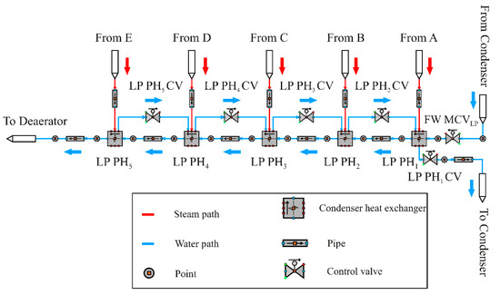
Figure 2.
LP feedwater model.
3.1. Feedwater Control Structures
To control the properties of the water (temperature and mass flow) in the feedwater loop during dynamic simulation, control loops must be set up to maintain the nominal limits of these properties for the feedwater and steam. Hence, several control circuits are modelled in the feedwater circuit in order to obtain an acceptable response during the fluctuations in the operating conditions.
3.1.1. Feedwater Main Control Valve in the LP Feedwater Circuit (FW MCVLP)
The feedwater main control valve at the feedwater circuit inlet adjusts the mass flow of water through the feedwater circuit. This valve is located before the first LP preheater (LP PH1), as depicted in Figure 3. The operation mode of FW MCVLP is clarified below:
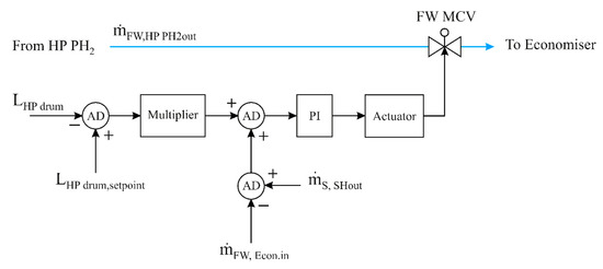
Figure 3.
Feedwater main control valve in the LP feedwater circuit (simplified).
At the inlet of the feedwater circuit, the mass flow data of the water is recorded, and a control signal is sent for comparison with the setpoint (44 kg/s). This comparison is performed by means of PI controller that sends the signal to the actuator, which in turn operates the FW MCVLP.
3.1.2. LP Preheater Level Controllers
Changes in the levels of the shell side for the LP preheaters are caused due to steam extractions from the turbine. Therefore, these levels of condensed water in the shell side are controlled using fife LP preheaters control valves (LP PH1 CV1—LP PH1 CV5). The locations of the LP preheater control valves are illustrated in Figure 4. The operation mode of LP PH level control circuits can be described in the three steps as follows:
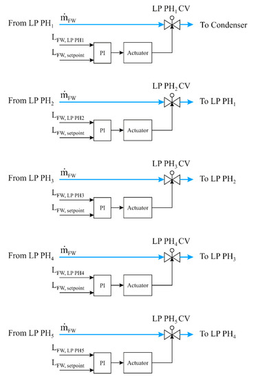
Figure 4.
LP preheater level controllers (simplified).
- The disparity between the real level and level setpoint of water in the shell side is measured.
- PI controller commands the actuator.
- The actuator operates the LP PH control valve in order to achieve the setpoint value.
4. Boiler Model
The boiler circuit starts from the HP preheaters (HP PH1, HP PH2) with a pressure of 109 bar and ends with the generation of steam at the outlet of the superheaters with a pressure of 106 bar, as previously demonstrated in Figure 5. However, the water enters the tubes side of HP preheaters by boiler pumps. Thereafter, the HP steam extractions is condensed on the shell side of HP preheaters. Although extracting steam to heat the feedwater reduces the power production of the turbine, it also raises the temperature of the water going into the boiler, resulting in greater cycle efficiency.
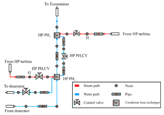
Figure 5.
Boiler model.
After heating the water in the HP preheaters, the water enters the economiser with a temperature of 250 °C and leaves it at a temperature of 311 °C due to the heat gained from the thermal oil. Thereafter, the saturation steam is generated in the HP tank by the water circulation and heat exchange between the thermal oil and feedwater. The water is circulated between the evaporators and HP tank using the high-pressure recirculation pump (HPRP). It should be mentioned here that the principle of operation of the high-pressure tank is a separator.
In the HP tank, the steam leaves to the superheaters while the hot water is recirculated again. In the superheaters, the saturation steam earns additional heat from the thermal oil. Here, the superheated steam enters the HP turbine at a temperature of 384 °C.
On the other hand, a part of HP steam expanded from the HP turbine (46 kg/s during the daytime hours and 41 kg/s in the evening hours) is used in the moisturise separator. Then it flows to the reheaters with a pressure approximately of 20.4 bar and a temperature of 214 °C. Thereafter, the reheated steam flows into the LP turbine at a temperature of 383 °C.
4.1. Boiler Control Structures
Important work has been conducted in this model, to implement, verify and improve control units that have to fulfil all essential functions. The application of suitable control procedures and the selection of realistic parameters for control circuits is essential to providing a high level of accuracy in these controllers in the dynamic simulation. To illustrate, the boiler circuit control procedures the controllers will be described in detail.
4.1.1. HP Preheater Level Control Circuits
Similar to what happens in LP preheaters, some oscillations occurred in the HP preheaters due to condense the steam extractions in the shell paths of these preheaters. The HP preheater level controllers keep the water levels in the shell side at constant values. Hence, there are two HP preheater control valves (HP PH1 CV and HP PH2 CV) that regulate the levels of water in the shell side. The locations of the HP preheater control valves are demonstrated in Figure 6. The operation mode of HP PH level control circuits is similar to the operation mode of control valves in the LP preheaters.
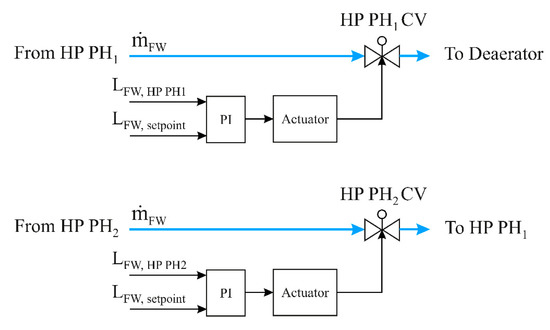
Figure 6.
HP preheater level controllers (simplified).
4.1.2. HP Drum Level Controller
During the start-up and the hard steam turbine transient, the mass flow rates at the entrances and the exits of the evaporators are highly deflected. It is clear that the water swelling in the HP evaporators is involved. However, in the case of small drum volume, the incoming/outcoming mass flow rates oscillation produce drum level fluctuations. During the dynamic process, the HP drum controller follows the level fluctuations in the drum in order to regulate the feedwater mass flow coming to the HP drum and to maintain the water level at a preset value. The procedures of this controller can be divided into three cases depending on three operating periods (i.e., normal load, shutdown and start-up periods). The feedwater coming to the drum is adjusted using the HP feedwater main control valve (FW MCVHP). This control valve is installed between HP PH2 and the economisers, as demonstrated in Figure 7.
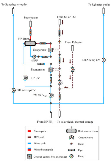
Figure 7.
Boiler model.
The procedures of this controller are a preset setpoint according to the operating period and compared with the measured data. The filling level of the high-pressure drum is gauged and checked against the setpoint (depending on the operating case). The difference ( between the setpoint and the measured point is recorded and is sent a control signal to the PI controller. The controller’s output range is specified between (0 and 100) in this model. Thereafter, the variation of mass flow rate is recorded between the steam mass flow at the SH exit and the feedwater mass flow rate at the inlet of the economiser . These differences (∆ṁ and ∆L) are compared and the readings are sent to a PI controller, which in turn directs the actuator to control the aperture of (FW MCVHP).
4.1.3. Economiser’s Bypass Controller (EBP CV)
The economiser’s bypass control valve (EBP CV) adjusts the feedwater temperature at the outlet of the economiser to lower than the boiling temperature by a preset value, as described in Figure 8. This process is carried out by passing a portion of feedwater from the inlet of the economiser to the drum in order to maintain a stable flow into the HP evaporators. The principle of work for the EBP CV will be explained as follows:
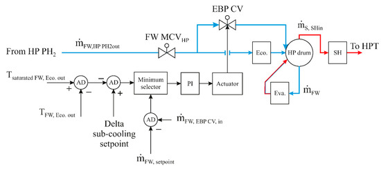
Figure 8.
Economiser’s bypass controller (simplified).
- The saturated temperature of feedwater at the HP economiser outlet is measured and compared with the real temperature at the HP economiser outlet.
- Deviation between both temperatures is compared with the HP delta sub-cooling (5 °C). However, the user can easily define any other needed value depending on the demand.
- The output signal from the second comparator (AD) enters a minimum selector and then sends a PI controller.
- The PI controller sends the commands to the actuator, which regulates the feedwater temperature through the economiser’s bypass control valve (EBP CV).
When the HP economiser bypass valve reaches its maximum mass flow limit, the PI will be directed through the variation between the bypass mass flow and the maximum setpoint of 8 kg/s (could vary by the user) for preventing any further increase in the bypass mass flow rate.
4.1.4. SH and RH Attemperator Controllers
The superheated steam and reheated steam temperatures are regulated to the desired value (384 °C) using two controllers (superheater attemperator and reheater attemperator). A portion of water is injected into the superheater and reheater inlet to adjust the inlet temperature of HP and LP turbines, respectively. Each attemperator control valve has a control circuit, which operates independently of the other. The operation mode of both attemperator controllers is the same, and it can be described as follows: A comparator checks the variation of steam temperatures between the setpoint (384 °C) and at the HP superheater outlet. This difference signal is sent to the PI controller. After that, the actuator is directed by the PI controller to operate the SH and RH attemperator control valves, as displayed in Figure 9.
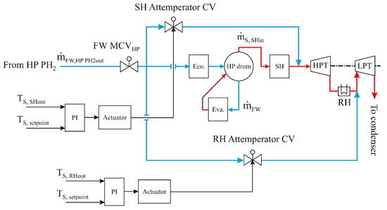
Figure 9.
SH and RH attemperator controllers (simplified).
5. Steam Turbine Model
The steam turbine is modelled based on two pressure sections. The first one includes two HP stages and the second one consists of six LP stages. In addition, a reheat process is added after the last second HP stage and before the first LP stage. Furthermore, eight portions of steam are extracted from the HP and LP turbine stages, as illustrated in Figure 10. The HP superheated steam enters the HP turbine with a temperature of 384 °C and a pressure of 106 bar. The steam then leaves the high-pressure turbine at a rate of 50 kg/s and extracts about 5 kg/s of steam from the HP-PH2. At the exit of the high-pressure turbine, the partly released steam (4 kg/s) passes into the HP-PH1, and the remainder of the released high-pressure steam (46 kg/s) flows into the moisture separator; it then proceeds to enter the reheaters with a temperature of 215 °C and a pressure of 20.5 bar. As shown earlier, the temperature of the reheated steam is controlled to about 383 °C through the RH attemperator with the help of high-pressure feedwater. The reheated steam is then fed into the LP-turbine. During LP turbine stages, there are five steam extractions that enter the LP preheaters in the feedwater circuit and one extraction enters the deaerator. Subsequently, the completely exhausted steam flows out of the LP-turbine to the condenser with a temperature of about 30 °C. It condenses the totally released steam from the LP-turbine, after which the PTPP cycle is restarted.
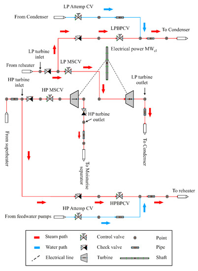
Figure 10.
Steam turbine model.
5.1. Steam Turbine Control Structures
Several control circuits should be installed in the steam turbine net in order to obtain the desired steam properties. However, the steam turbine model consists of the following six control circuits. Therefore, the steam turbine control circuits will be explained in the following sections.
5.1.1. LP Bypass Controller and LP Main Steam Control Valve
LP bypass control circuit contains two control valves, as displayed in Figure 11 and Figure 12. The LP main steam control valve (LP MSCV) adjusts the flow to the LP turbine. It is controlled by a time gradient (polyline). During standard operation, the HP-MSCV must be opened, and during the start-up phase, it must be closed. The LP bypass control valve (LP BPCV) is operated using a summation rule. In this case, the two control functions are to be performed in two different ways. On the one hand, the undesired steam must be diverted to the condenser. On the other hand, the second task is that the reheated steam pressure must be regulated to a certain setpoint pressure initially, with a maximum pressure that must not be exceeded. Moreover, when the steam turbine trip occurs, LP BPCV is operated to bypass the entire steam. The high pressure main steam control valve HP MSCV is operated in the same way as the (LP MSCV) by a time gradient (polyline).
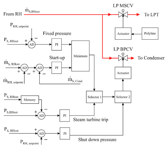
Figure 11.
LP bypass controller and LP main steam controller (simplified).
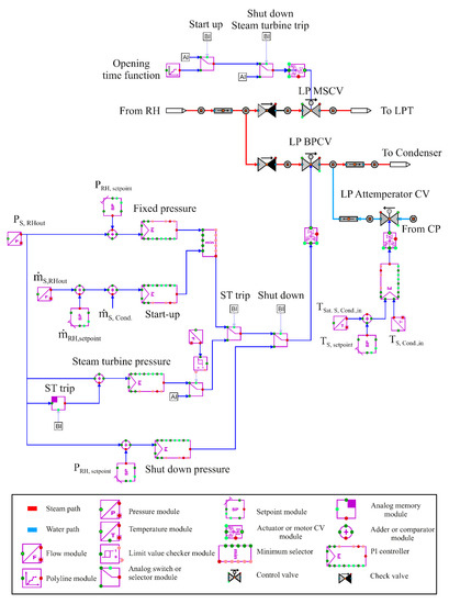
Figure 12.
LP bypass controller and LP main steam controller (APROS model).
5.1.2. LP Attemperator Control Valve (LP Attemp CV)
An LP attemperator controller was modelled to cool the bypassed steam after the LP BPCV, as shown in Figure 13. This cooler cools the bypassed steam to 50 °C higher than the saturated steam temperature before it enters the condenser. It should be mentioned here that water coming from condenser pump (CP) is used in the LP attemperator.
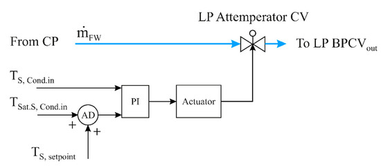
Figure 13.
LP attemperator control valve (LP Attemp CV) (simplified).
5.1.3. HP Attemperator Control Valve (HP Attemp CV)
An HP attemperator controller was built to provide cooling of the bypassed steam downstream of the HP BPCV to 50 °C higher than the saturated steam temperature before entering the reheater. This cooling process is achieved by the water, which is pumped from the boiler feedwater pump (BFP) into the HP BPCV outlet, as demonstrated in Figure 14.
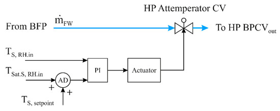
Figure 14.
HP attemperator control valve (HP Attemp CV) (simplified).
6. Condenser Model
The completely released steam exits the steam turbine at pressure of 0.05 bar and temperature 30 °C. It should be mentioned here that the steam mass flow rate enters the condenser with mass flow of 34.4 kg/s during the daytime and at 30.6 kg/s in the night. Based on cooling water coming from the cooling water pumps at a pressure of 2 bar and a temperature of 19 °C, the condenser condenses the completely discharged steam from the LP turbine into water. This process of cooling is performed by a cooling water mass flow rate of 2344 kg/s. The cooling water then flows back into the cooling tower at a temperature of 27 °C. Finally, the steam extracted from the LP turbine are condensated and accumulated in the LP preheaters (9.6 kg/s during the day and 8.6 kg/s at night), and mixes with the condensate water in the condenser. Herein, this mixture is pumped by means of the condenser pumps (CP) with mass flow of 44 kg/s during the daytime or 39.2 kg/s in the evening hours and then it enters the LP PH1 at a pressure of 18.7 bar and a temperature of 37 °C.
6.1. Condenser Control Structures
In the condenser model, there is one control valve, namely the cooling water control valve (CWCV). It will be described in the following section.
Cooling Water Control Valve (CWCV)
The cooling water control valve regulates the temperature of condensate water in the condenser. This valve is located between the condenser (tube side) and the cooling water source, as demonstrated in Figure 15. The operation mode of CWCV is outlined below:
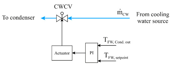
Figure 15.
Cooling water control valve (CWCV) (simplified).
The condensed water temperature at the condenser outlet is recorded and checked against the set point (37 °C). This comparison is implemented by a PI controller that sends the control signal to the actuator, which in turn operates the CWCV.
Finally, it should be mentioned here that the predictions of the power block have been validated versus experimental data from the 50 MWel Andasol II power plant in Spain during the summer days. The comparison showed a very good agreement with the measured data, as illustrated in Figure 16 [33].
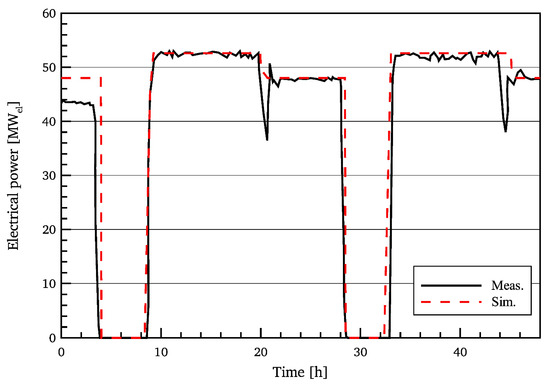
Figure 16.
Comparison of the measured total electrical power with the simulated results for 13 and 14 July 2010.
7. Conclusions
Based on the real engineering data and specifications of a real power plant (Andasol II) in Spain, a comprehensive dynamic model of a PB is implemented. In this study, a detailed description for the advanced controllers used in the power block of a 50 MWel parabolic trough power plant is presented. The implemented model includes four main parts, namely the LP feedwater circuit, the boiler, steam turbine and condenser as well as the control structures for each part. The components of the power block model have been accurately described and built using APROS. The power block produces maximum electrical power of 52.5 MWel in the daytime hours and 48 MWel in the night period. The objective of this study was to build reference models for PB, which in turn will provide researchers and designers with a better understanding of the state of advanced control loops in these power plants. Furthermore, such models will be able to determine the most appropriate way to operate the power plant. Additionally, it should be mentioned here that what distinguishes the APROS program is the high dynamic and fast response to fluctuations that occur during long and short periods of operation, unlike the rest of the programs used. It also contains many components of control circuits in addition to the main components of the power plants such as turbines, compressors, pumps, etc. Moreover, APROS contains statistical data for different latitude and longitude, in addition to the different days of the year.
Author Contributions
Methodology, W.A.K.A.-M., A.S.H. and H.M.H.A.-K.; software, W.A.K.A.-M.; investigation, W.A.K.A.-M., A.S.H. and H.M.H.A.-K.; writing—original draft preparation, W.A.K.A.-M.; writing—review and editing, W.A.K.A.-M. and F.A.; supervision, B.E. All authors have read and agreed to the published version of the manuscript.
Funding
This research received no external funding.
Informed Consent Statement
Not applicable.
Data Availability Statement
Not applicable.
Acknowledgments
We acknowledge support from the Deutsche Forschungsgemeinschaft (DFG—German Research Foundation) and the Open Access Publishing Fund of the Technical University of Darmstadt. The first author would like also to thank the University of Technology- Iraq.
Conflicts of Interest
All authors declare no conflict of interest.
Nomenclature
| h | Enthalpy [kJ/kg] |
| ṁ | Mass flow rate [kg/s] |
| P | Pressure [bar] |
| T | Temperature [°C] |
| t | Time [sec] |
| u | Velocity [m/s] |
| ρ | Density [kg/m3] |
| DNI | Direct normal irradiation [W/m2] |
Abbreviations
| AD | Adder |
| APROS | Advanced process simulation software |
| BFP | Boiler feedwater pump |
| CP | Condenser pump |
| FW | Feedwater |
| HP | High pressure |
| HTF | Heat transfer fluid |
| LP | Low pressure |
| PB | Power block |
| PTPP | Parabolic trough power plant |
| PI | Proportional–integral controller |
| SF | Solar field |
| TSS | Thermal storage system |
| SP | Set point |
| TI | Temperature measurement component |
References
- Müller-Steinhagen, H. FaTF. Concentrating Solar Power. A Review of the Technology; Institute of Technical Thermodynamics, German Aerospace Centre: Stuttgart, Germany, 2004; p. 9. [Google Scholar]
- Kaygusuz, K. Prospect of concentrating solar power in Turkey: The sustainable future. Renew. Sustain. Energy Rev. 2011, 15, 808–814. [Google Scholar] [CrossRef]
- Bhutto, A.W.; Bazmi, A.A.; Zahedi, G.; Klemeš, J.J. A review of progress in renewable energy implementation in the Gulf Cooperation Council countries. J. Clean. Prod. 2014, 71, 168–180. [Google Scholar] [CrossRef]
- Wahhab, H.A.A.; Al-Maliki, W.A.K. Application of a Solar Chimney Power Plant to Electrical Generation in Covered Agricultural Fields. IOP Conf. Ser. Mater. Sci. Eng. 2020, 671, 012137. [Google Scholar] [CrossRef]
- Artola, V.; María, J. Performance of a 50 MW Concentrating Solar Power Plant. Master’s Thesis, Politecnico Di Bari, Bari, Italy, 2010. [Google Scholar]
- Desai, N.B.; Bandyopadhyay, S. Optimization of concentrating solar thermal power plant based on parabolic trough collector. J. Clean. Prod. 2015, 89, 262–271. [Google Scholar] [CrossRef]
- Fernández-García, A.; Rojas, E.; Pérez, M.; Silva, R.; Hernández-Escobedo, Q.; Manzano-Agugliaro, F. A parabolic-trough collector for cleaner industrial process heat. J. Clean. Prod. 2015, 89, 272–285. [Google Scholar] [CrossRef]
- Sharan, P.; Bandyopadhyay, S. Solar assisted multiple-effect evaporator. J. Clean. Prod. 2016, 142, 2340–2351. [Google Scholar] [CrossRef]
- Teske, S.L.J.; Crespo, L.; Bial, M.; Dufour, E.; Richter, C. Solar Thermal Electricity, Global Outlook 2016; Greenpeace International: Amsterdam, The Netherlands, 2016. [Google Scholar]
- Reddy, K.; Kumar, K.R. Solar collector field design and viability analysis of stand-alone parabolic trough power plants for Indian conditions. Energy Sustain. Dev. 2012, 16, 456–470. [Google Scholar] [CrossRef]
- Chacartegui, R.; Vigna, L.; Becerra, J.; Verda, V. Analysis of two heat storage integrations for an Organic Rankine Cycle Parabolic trough solar power plant. Energy Convers. Manag. 2016, 125, 353–367. [Google Scholar] [CrossRef]
- Zhang, H.; Baeyens, J.; Degrève, J.; Cacères, G. Concentrated solar power plants: Review and design methodology. Renew. Sustain. Energy Rev. 2013, 22, 466–481. [Google Scholar] [CrossRef]
- Lovegrove, K.; Stein, W. Concentrating Solar Power Technology: Principles, Developments and Applications; Elsevier: Amsterdam, The Netherlands, 2012. [Google Scholar]
- Wagner, P.H.; Wittmann, M. Influence of different operation strategies on transient solar thermal power plant simulation models with molten salt as heat transfer fluid. Energy Procedia 2014, 49, 1652–1663. [Google Scholar] [CrossRef][Green Version]
- Weber, G.; Di Giuliano, A.; Rauch, R.; Hofbauer, H. Developing a simulation model for a mixed alcohol synthesis reactor and validation of experimental data in IPSEpro. Fuel Processing Technol. 2016, 141, 167–176. [Google Scholar] [CrossRef]
- Zamarreño, J.M.; Mazaeda, R.; Caminero, J.A.; Rivero, A.J.; Arroyo, J.C. A new plug-in for the creation of OPC servers based on EcosimPro© simulation software. Simul. Model. Pract. Theory 2014, 40, 86–94. [Google Scholar] [CrossRef]
- Malinowski, L.; Lewandowska, M.; Giannetti, F. Design and analysis of a new configuration of secondary circuit of the EU-DEMO fusion power plant using GateCycle. Fusion Eng. Des. 2018, 136, 1149–1152. [Google Scholar] [CrossRef]
- Bordignon, S.; Emmi, G.; Zarrella, A.; De Carli, M. Energy analysis of different configurations for a reversible ground source heat pump using a new flexible TRNSYS Type. Appl. Therm. Eng. 2021, 197, 117413. [Google Scholar] [CrossRef]
- Eck, M.; Hirsch, T. Dynamics and control of parabolic trough collector loops with direct steam generation. Sol. Energy 2007, 81, 268–279. [Google Scholar] [CrossRef]
- Greenhut, A.D.; Tester, J.W.; DiPippo, R.; Field, R.; Love, C.; Nichols, K.; Augustine, C.; Batini, F.; Price, B.; Gigliucci, G. Solar–geothermal hybrid cycle analysis for low enthalpy solar and geothermal resources. In Proceedings of the World Geothermal Congress, Bali, Indonesia, 25–29 April 2010. [Google Scholar]
- García, I.L.; Álvarez, J.L.; Blanco, D. Performance model for parabolic trough solar thermal power plants with thermal storage: Comparison to operating plant data. Sol. Energy 2011, 85, 2443–2460. [Google Scholar] [CrossRef]
- Ehrhart, B.; Gill, D. Evaluation of annual efficiencies of high temperature central receiver concentrated solar power plants with thermal energy storage. Energy Procedia 2014, 49, 752–761. [Google Scholar] [CrossRef]
- Chennaif, M.; Maaouane, M.; Zahboune, H.; Elhafyani, M.; Zouggar, S. Tri-objective techno-economic sizing optimization of Off-grid and On-grid renewable energy systems using Electric system Cascade Extended analysis and system Advisor Model. Appl. Energy 2022, 305, 117844. [Google Scholar] [CrossRef]
- Al-Maliki, W.A.K.; Al-Hasnawi, A.G.T.; Abdul Wahhab, H.A.; Alobaid, F.; Epple, B. A Comparison Study on the Improved Operation Strategy for a Parabolic trough Solar Power Plant in Spain. Appl. Sci. 2021, 11, 9576. [Google Scholar] [CrossRef]
- Al-Maliki, W.A.K.; Mahmoud, N.S.; Al-Khafaji, H.M.; Alobaid, F.; Epple, B. Design and Implementation of the Solar Field and Thermal Storage System Controllers for a Parabolic Trough Solar Power Plant. Appl. Sci. 2021, 11, 6155. [Google Scholar] [CrossRef]
- Ho, C.K. Software and Codes for Analysis of Concentrating Solar Power Technologies; Sandia Report; Sandia National Laboratories: Albuquerque, NM, USA, 2008. [Google Scholar]
- Liu, S.; Faille, D.; Fouquet, M.; El-Hefni, B.; Wang, Y.; Zhang, J.; Wang, Z.; Chen, G.; Soler, R. Dynamic simulation of a 1MWe CSP tower plant with two-level thermal storage implemented with control system. Energy Procedia 2015, 69, 1335–1343. [Google Scholar] [CrossRef]
- Mitterhofer, M.; Orosz, M. Dynamic Simulation and Optimization of an Experimental Micro-CSP Power Plant. In Proceedings of the Energy Sustainability, Bangkok, Thailand, 25–26 October 2015; p. V001T005A007. [Google Scholar]
- Ma, L.; Zhang, T.; Zhang, X.; Wang, B.; Mei, S.; Wang, Z.; Xue, X. Optimization of parabolic trough solar power plant operations with nonuniform and degraded collectors. Sol. Energy 2021, 214, 551–564. [Google Scholar] [CrossRef]
- Al-Maliki, W.A.K.; Alobaid, F.; Keil, A.; Epple, B. Dynamic Process Simulation of a Molten-Salt Energy Storage System. Appl. Sci. 2021, 11, 11308. [Google Scholar] [CrossRef]
- Ferruzza, D.; Topel, M.; Laumert, B.; Haglind, F. Optimal start-up operating strategies for gas-boosted parabolic trough solar power plants. Sol. Energy 2018, 176, 589–603. [Google Scholar] [CrossRef]
- El Hefni, B. Dynamic modeling of concentrated solar power plants with the ThermoSysPro library (Parabolic Trough collectors, Fresnel reflector and Solar-Hybrid). Energy Procedia 2014, 49, 1127–1137. [Google Scholar] [CrossRef]
- Al-Maliki, W.A.K.; Alobaid, F.; Kez, V.; Epple, B. Modelling and dynamic simulation of a parabolic trough power plant. J. Process Control 2016, 39, 123–138. [Google Scholar] [CrossRef]
- Zhang, S.; Liu, M.; Zhao, Y.; Liu, J.; Yan, J. Dynamic simulation and performance analysis of a parabolic trough concentrated solar power plant using molten salt during the start-up process. Renew. Energy 2021, 179, 1458–1471. [Google Scholar] [CrossRef]
- Yazdi, M.; Manesh, M.H.K. Dynamic 6E analysis of direct steam generator solar parabolic trough collector power plant with thermal energy storage. Sustain. Energy Technol. Assess. 2022, 49, 101759. [Google Scholar] [CrossRef]
- Yuanjing, W.; Cheng, Z.; Yanping, Z.; Xiaohong, H. Performance analysis of an improved 30 MW parabolic trough solar thermal power plant. Energy 2020, 213, 118862. [Google Scholar] [CrossRef]
- Montañés, R.M.; Windahl, J.; Pålsson, J.; Thern, M. Dynamic modeling of a parabolic trough solar thermal power plant with thermal storage using modelica. Heat Transf. Eng. 2018, 39, 277–292. [Google Scholar] [CrossRef]
- Silva, R.; Pérez, M.; Fernández-Garcia, A. Modeling and co-simulation of a parabolic trough solar plant for industrial process heat. Appl. Energy 2013, 106, 287–300. [Google Scholar] [CrossRef]
- Alobaid, F. Start-up improvement of a supplementary-fired large combined-cycle power plant. J. Process Control 2018, 64, 71–88. [Google Scholar] [CrossRef]
- Alobaid, F.; Mertens, N.; Starkloff, R.; Lanz, T.; Heinze, C.; Epple, B. Progress in dynamic simulation of thermal power plants. Prog. Energy Combust. Sci. 2017, 59, 79–162. [Google Scholar] [CrossRef]
- Harlow, F.H.; Welch, J.E. Numerical calculation of time-dependent viscous incompressible flow of fluid with free surface. Phys. Fluids 1965, 8, 2182–2189. [Google Scholar] [CrossRef]
- Hänninen, M. Phenomenological Extensions to APROS Six-Equation Model. Non-Condensable Gas, Supercritical Pressure, Improved CCFL and Reduced Numerical Diffusion for Scalar Transport Calculation; VTT Publications 720; KULKAISIJA-UTGIVARE-PUBLISHER: Espoo, Finland, 2009. [Google Scholar]
- Siikonen, T. Numerical method for one-dimensional two-phase flow. Numer. Heat Transf. Part A Appl. 1987, 12, 1–18. [Google Scholar]


Publisher’s Note: MDPI stays neutral with regard to jurisdictional claims in published maps and institutional affiliations. |
© 2021 by the authors. Licensee MDPI, Basel, Switzerland. This article is an open access article distributed under the terms and conditions of the Creative Commons Attribution (CC BY) license (https://creativecommons.org/licenses/by/4.0/).