Abstract
Renewable integration into the electricity system of Great Britain (GB) is causing considerable demand for additional flexibility from plants. In particular, a considerable share of this flexibility may be dispatched to secure post-fault transient frequency dynamics. Pursuant to the unprecedented changes to the traditional portfolio of generation sources, this work presents a detailed analysis of the potential system-level value of unlocking flexibility from nuclear electricity production. A rigorous enhanced mixed integer linear programming (MILP) unit commitment formulation is adopted to simulate several generation-demand scenarios where different layers of flexibility are associated to the operation of nuclear power plants. Moreover, the proposed optimisation model is able to assess the benefit of the large contribution to the system inertial response provided by nuclear power plants. This is made possible by considering a set of linearised inertia-dependent and multi-speed constraints on post fault frequency dynamics. Several case studies are introduced considering 2050 GB low-carbon scenarios. The value of operating the nuclear fleet under more flexible paradigms is assessed, including environmental considerations quantified in terms of system-level CO2 emissions’ reduction.
1. Introduction
The integration of large shares of Variable Renewable Energy Sources (VRES) into the electricity system of Great Britain (GB) is changing the way the power system is operated. This is mainly since an increasing number of conventional synchronous generators are being displaced by VRES, whose ability to contribute to the security of the system is reduced [1]. Operating the system with fewer conventional synchronous power plants implies a sharp reduction in the available inertial response. In their typical configuration, VRES do not naturally provide inertial response nor automatic primary frequency control [1,2], leading the system operator, responsible for the secure operation of the network, to require large amounts for frequency response services [3,4,5,6]. In fact, the demands on frequency response depend on the available inertia, the largest possible infeed loss (which is not expected to change [7]) and the speed in the provision of frequency response services. It is, therefore, also important to consider technologies capable of providing inertial response [2,8,9,10,11] and new ancillary services, namely Enhanced Frequency Response (EFR) [7,12,13,14,15], in any analysis. In addition to the challenges associated with higher levels of VRES, there is an increased desire from policymakers from many countries, including the UK, to electrify more of current non-electric demand (for example transport) to aid with decarbonisation targets for the year 2050 [16,17].
The methodology and scope of this investigation is focused on determining the post-fault behaviour of the electricity transmission system and, by acknowledging technical services of each technology (e.g., primary response and enhanced frequency response), we aim to ensure system-level security. It is worth noting that, in the event system-level security is not ensured and results in demand disconnection (i.e., blackouts), separate analyses would need to be performed to model how technologies connected to the system (including nuclear power plants) would be used to re-energise the system.
1.1. Related Work
Previous works [16,18,19,20,21,22] have assessed the future UK electricity system with large shares of renewables. However, the interplay between inertial dependent frequency constraints and the actual cost-based system commitment/dispatch decisions is neglected.
Following a different fundamental approach, other works have focused on the assessment of frequency response requirements considering, up to certain differences, the amount of available inertial response and the speed of provision of frequency response. The authors in Reference [23] have introduced a set of linear constrains to define sufficient conditions for primary response adequacy. However, an ex-ante dispatch decision was adopted, making the available inertial response a pre-determined quantity, i.e., not a decision variable of the optimisation problem. Furthermore, effective formulations have been introduced in Reference [24,25,26,27]. Regardless of the fundamental differences among these works, it is possible to highlight a common trait: the inertial response and its effect of post-fault frequency dynamics becomes a decision variable of a Unit Commitment (UC) problem. Therefore, the optimal amount of frequency response acknowledges the interplay between inertial response and primary response from conventional generators.
More recently, the authors in Reference [7,28] extended the inertia-dependent frequency constraints by letting the underlying UC recognise the different speeds in the provisions of frequency response associated with conventional generators (5–10 s) and flexible assets, e.g., battery storage. Similar setups have been presented in Reference [29,30,31].
The above mentioned works have brought exceptional understanding regarding the interplay between secure frequency dynamics and cost-effective generation-demand balance. However, two fundamental aspects of future power systems have not been fully considered. The first regards the valuable role of inertial response. The synchronous generators of nuclear power plants are large providers of inertial response. However, technical constraints may limit the flexibility in the operation of these units, especially with respect to the provision of primary response and operations, for instance, characterised by dispatch levels far from the maximum capacity of the plant. In fact, the above-mentioned studies did not fully assess the potential benefits of nuclear flexibility. The second aspect is with respect to the power system scenarios considered. In fact, the push towards the electrification of the transport sectors, together with the changes to the typical demand profiles introduced by electric vehicles, have not been fully accounted for in the literature.
1.2. Contribution
This study contributes to the existing relevant literature by addressing the research gaps identified in the literature. In fact, based on the fundamental methodology proposed in Reference [7], this study aims at quantifying the potential benefits of nuclear operational flexibility for achieving security/stability in the power system under high electrification scenarios (around 570 TWh compared with current consumption of around 300 TWh in the UK [16]). Furthermore, in this work, we aim to study different scenarios with varying levels of nuclear, fossil fuels and VRES to determine not only the feasibility of the scenarios under steady-state and transient conditions but also the benefits of different storage and operational flexibility mechanisms provide. In particular, there is a focus in this study on the services the nuclear plants are providing and their operating characteristics (including number of shutdowns and capacity factors). These characteristics were not studied in previous works.
To address the above we firstly provide details on the scenarios considered and the assumptions around the technologies employed (e.g., batteries providing EFR, interconnectors, nuclear, VRES, etc.). Then, starting from a nominal energy mix consisting of nuclear (27% of average generation), semi-base units (37% of average generation comprising predominantly gas but also biomass) and VRES (23% of average generation), three distinct cases were studied. The cases studied were: (1) nuclear plants are assumed to be inflexible and do not operate below 98% of nominal power; (2) nuclear plants are able to operate flexibly with minimum stable factors of 55%; and (3) the semi-base gas plants in the nominal energy mix are replaced with nuclear or VRES while allowing flexible operation of nuclear plants in both cases. In all scenarios studied, the boundary conditions for interconnectors come from a pan-European model to reasonably estimate the ability of other countries to supply the UK with electricity, and we assume around 12.6 million electric vehicles are deployed which can provide demand side management in the form of delaying onset of charging. Furthermore, sensitivity analyses are performed with nuclear plants having minimum stable factors down to 20% of nominal power.
In all cases the energy generation per technology type, carbon dioxide emissions, frequency response and system-level inertia are investigated. In this context, the study and method adopted aims to match the technical constraints of conventional generators, including new nuclear, in-line with optimised requirements for frequency response and inertial response described in the methodology outlined in Reference [7].
2. Scenarios and Assumptions
2.1. Demand and Generation Mix
The main assumptions for this study are based on the EU SysFlex European project [32]. High future electrification scenarios consistent with 2050 Pathways, as described in Reference [33], were modelled. Each simulation solves daily unit commitment problems that give an hourly view of the ability of generation units to meet demand. In addition, system constraints (as outlined in this section) relating to post-fault frequency recovery with an hourly granularity for the year 2050 are modelled to assess system security.
2.1.1. Demand and VRES Profile
For the total annual electricity demand, 572 TWh has been chosen directly from Reference [33]. As shown in Table 1, this value is in the range of several scenarios provided. Note that this amount of demand is much higher than the 441 TWh from the Community Renewables scenario in the National Grid Future Energy Scenarios 2018 (FES) [22].

Table 1.
Annual electricity demand for 2050 [22,32,33].
The demand profile is directly taken from the EU SysFlex scenario with the highest total demand. A multiplier has been used to this profile to meet the 572 TWh from Reference [33]. The load factor profile of intermittent VRES (solar PV, as well as onshore and offshore wind) are also taken from the same EU SysFlex scenario.
Electricity consumption from Electric Vehicles (EVs) is included in the demand profiles (EU SysFlex considers 12.57 M EVs [32]—compared with current deployment of 57 k EV and 88 k hybrid vehicles according to Reference [22]). This level of EV deployment results in a total additional consumption of 33.68 TWh added to the demand profile. The model assumes that smart charging is adopted by the EV fleet, which involves charging at night in order to minimise peak demand; however, Vehicle to Grid (V2G) technology is not adopted. Note that a scenario with a higher number of EVs would induce possible higher ramping needs, which could also be smoothed using V2G or smart charging [34].
2.1.2. Generation Mix
The scenario describes projections for the year 2050. All assumptions on installed capacity are taken from EU SysFlex, except for the 17.3 GW of battery storage taken from Reference [22]. All technologies have been grouped by type: Base (Nuclear), Semi-base (CCGT (Combined Cycle Gas Turbine) and Biomass), Peak (Battery storage, Pump hydro storage, OCGT (Open Cycle Gas Turbine), and Interconnection), and Intermittent (Solar, Offshore, Onshore, and Hydro). Within the semi-base group, gas dominates with 39 GW of CCGT installed.
2.2. Technologies
The following technologies are modelled as an aggregation of multiple units with similar characteristics from variable cost and operation point of view:
- Nuclear: Nuclear units were modelled as units with 1500 MW capacity, not subsidised and with identical fuel prices. Variable assumptions are made regarding capability of provision of primary response and minimum stable factors (MSF)—that is the minimum amount of power the system can generate—to assess the importance of these attributes as outlined in the case studies described in Section 3.
- Semi-base and peaking plants: These technologies represent other conventional synchronous generators including Biomass, CCGT, OCGT, Gas and diesel reciprocating engines. The units are split into 500 MW and 300 MW plants to represent a greater diversity, with the same constant of inertia for every unit.
- Wind (Onshore & Offshore): In-house profiles are used, and curtailment costs are applied as negative variable cost (£/MWh).
- Solar PV: In-house profiles are used, and curtailment costs are applied as negative variable cost (£/MWh).
- Run of river hydro: In-house profiles are used, and curtailment costs are applied as a negative variable cost (£/MWh).
- Battery Storage: This technology is represented as one large 2 h storage system of 17.3 GW. Parameters that are used to model the operation of battery and hydro storage (c-rate, roundtrip efficiency) are taken from Reference [35].
- Pumped Hydro Storage (PHS): This technology is represented as two reservoirs and one corresponding turbine/pump for each system. Pump and turbine modes are exclusive. Minimum discharge power for PHS in both pump/turbine modes is taken from Reference [36].
- Interconnectors: Future interconnectors are modelled as aggregated interconnectors. The flows were fixed (and taken from EU SysFlex outputs that models a pan-European system) and acts as boundary conditions to the cases investigated; thereby giving realistic consideration to the ability to call upon generation from outside of the UK.
It is worth noting that additional analysis for high nuclear energy scenarios should factor in the life cycle analysis for the plants including operational periods, spent fuel management during operation and also decommissioning and final waste disposal, see References [37,38,39] for further details.
The grid code currently requires that all generators connected to the transmission network must be able to provide primary response [40]. Thus, we assume in the study that, in 2050, offshore/onshore wind technologies are able to provide Primary Response (PR); interconnector links have the capability to provide both PR and EFR [3,41,42] and nuclear units are assumed to be sufficiently flexible to operate part-loaded (for energy or PR needs) depending on the case being studied. Note that the MSF directly impacts the minimum frequency response requirement of a plant, with the higher the MSF, the lower the headroom available for providing PR.
2.3. Frequency Constraint and System-Level Data
Maintaining post-fault frequency dynamics above certain security thresholds in response to the maximum infeed generation loss is one of the key-responsibilities of system operators. To do so, National Grid in GB sets security standard and thresholds concerning transient frequency excursions. Figure 1 provides an illustrative overview of the current thresholds on post-fault frequency conditions:
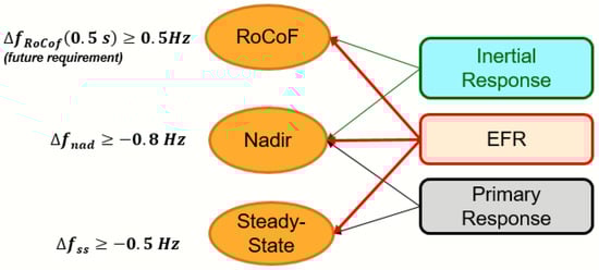
Figure 1.
Post-fault transient frequency conditions and security thresholds (left-hand side) associated with the relevant ancillary services (right-hand side).
- The first requirement concerns the Rate of Change of Frequency (RoCoF). This quantity is defined as the frequency variation that occurs over a certain measuring window. Current settings envisage the RoCoF to be maintained above 1 Hz/s, evaluated over a 0.5 s measuring window. In other words, frequency must not drop by more than 0.5 Hz in 0.5 s. This paper adopted the above-mentioned value concerning the RoCoF threshold. However, it is worth noting that the 1 Hz/s setting has been revised pursuant to the Accelerated Loss of Mains Change Programme [43]. In fact, the maximum RoCoF was limit was 0.125 Hz/s. Furthermore, maintaining the post-fault RoCoF above security thresholds prevents the activation of RoCoF-driven relays of the so-called Loss of Main protection schemes. These are typically installed on board of distribution-connected generators.
- Following an infeed generation loss, system frequency would reach its maximum deviation at the so-called nadir condition. In particular, the maximum frequency deviation is set to −0.8 Hz. It is important to maintain post-fault frequency nadir above this value in order to prevent the activation of costly and disruptive Low Frequency Demand Disconnection schemes.
- Finally, after the deployment of primary frequency control, the system frequency reaches the so-called quasi-steady state condition (i.e., frequency is no longer decreasing/increasing but has not yet recovered to its nominal value). The system operator requires that frequency remains above −0.5 Hz during the quasi-steady state condition.
The system operator ensures the respect of the transient security thresholds on frequency deviation discussed above by requiring the allocation of three ancillary services. The first one is the inertial response naturally provided by synchronous generators. As explained in Figure 1, the provision of inertial response contributes to containment of the RoCoF and the nadir. However, the limited kinetic energy reservoir associated with the inertial response does not allow a longer lasting support up to the quasi-steady state condition. The second service is the EFR. Typical providers of EFR are battery storage assets that automatically react to frequency changes by varying the power output within 1 s. Because of the rapidity requested to deliver such service, EFR contributes to all three frequency conditions. Finally, PR is provided by conventional generators by increasing their dispatch level in response to frequency changes. The delivery time of PR is 10 s. The slower nature of the delivery of this service limits the contribution of PR to the nadir and quasi-steady state conditions only.
Following the peer-reviewed methodology developed in Reference [7] (which has been applied in looking at nearer-term 2030 energy systems [25]), the post-fault frequency recovery leads to a set of constraints linking the total system inertia (H) the total primary response (R) and the total enhanced frequency response (E). The mathematical conditions are presented below.
Pursuant to the sudden and maximum generation loss [MW], the transient evolution of the network frequency is evaluated by means of the first-order ordinary differential Equation (1):
At the generic time step t, the natural damping characteristic of the load [MW] is expressed through the damping constant D [Hz−1]. The total (post-fault) inertia at step t, [MWs], is expressed in Equation (2).
In Equation (2), represents the constant of inertia [s] of the generic synchronous machine g, whose rated capacity is [MW]. The commitment decision is expressed by means of the binary variable , which assumes value 1 if the plant is online and 0 otherwise. It is worth noting that the inertial response corresponding to the faulted generator is subtracted from the available post-fault system inertia (being the constant of inertia related to ). Finally, in Equation (2), Hz and represents the nominal frequency.
Furthermore, the dynamics of the provision of EFR differ from those characterising PR. The first service is fully delivered within s, whereas the delivery interval for PR is s, with a non-negligible delay (e.g., 1 s) affecting its onset. In order to acknowledge these features, the differential Equation (1) is split into two separate models which are applied to different time intervals. The first case is presented in Equation (3), where only a linear increase in EFR up to is modelled, whereas the PR contribution is nil; hence, this model pertains the time interval .
Equation (4) describes the second model, which is valid for . After , the full amount of allocated EFR has been delivered. Hence, the provision of PR linearly increases up to .
Since holds (see Figure 1), the proposed constraint on the maximum RoCoF would require only the use of the differential Equation (3). In particular, Equation (5) is derived by integrating the differential Equation (3), imposing an initial condition and setting . Following the described calculations, Equation (5) is the numerator of a fraction which has as the denominator. Since the latter can only assume strictly positive values, the application of Equation (5) is sufficient to constrain the post-fault RoCoF. Note that s and represents the measuring window time for the RoCoF threshold in accordance with the description in Figure 1.
The methodology to effectively constrain the post-fault frequency nadir is more complex than the one adopted for the RoCoF. The complexity is due to the non-linear nature of the constraint on the nadir, which explicitly depends on the optimal combination of H, E and R. Moreover, based on such combination, the nadir can actually occur before or after , requiring both differential Equations (3) and (4) to be considered. In other words, for each of the two models (Equations (3) and (4)), a relevant nadir constraint has to be computed. However, regardless the particular dynamic model employed, the same fundamental steps have to be followed.
First, the relevant differential equation is integrated for a specified initial condition. Afterwards, a minimum condition is found by imposing the first-order derivative of the resulting frequency evolution to equal zero (). This equation is solved for t to then obtain an expression of as function of the relevant decision variables. The resulting expression of is inserted in the time evolution of the system frequency, i.e., . The nadir condition is eventually obtained by imposing that being , the maximum frequency deviation in Figure 1.
In the following we distinguish among two cases concerning the development of a nadir constraint for the relevant dynamic model (Equations (3) and (4)).
Case a, where : the condition is satisfied if and only if Equation (6) holds.
In accordance with the information concerning the RoCoF constraint (Equation (5)), the dynamic model (Equation (3)) only depends on the combination of and since PR is not yet deployed before . The applicable initial condition for the integration of the model in Equation (3) is once again . Note that is the unique solution of the monotonically decreasing function outlined in Equation (7), for any given value of and .
Case b, : The applicable frequency dynamic model is the differential Equation (4). In order to respect the continuity of the frequency evolution when time crosses , the initial condition to integrate Equation (4) is the value of the frequency deviation obtained by integrating the dynamic model in Equation (3). In particular the initial condition is given in Equation (8).
Having this in mind and following the steps indicated above concerning the derivation of a nadir constraint, the relevant constraint on the nadir valid if is expressed in Equation (9). This equation depends on all the three decision variables , , and .
As explained above, the two constraints on nadir (Equations (6) and (9)) are both non-linear. However, it has to be noted that Equation (6) is a convex function for all possible values of , . By introducing a number of couples , Equation (6) is linearised via a set of piecewise linear functions such that . The expression of the functions are given in Equation (11).
It is worth pointing out that the functions and are the first order partial derivatives of Equation (6) with respect to the variables and .
Similar considerations apply with respect to the nadir constraint (Equation (9)). As expressed in Equation (12), the linearisation process now considers a number of triples and a set of piecewise linear functions such that .
Once again, , and are the first order partial derivatives of Equation (9) with respect to , , and , individually.
Although two different nadir constraints had to be developed following from the two differential Equations (3) and (4), the unit commitment optimisation model applies constraint Equation (6), i.e., its linearised version (Equation (11)), or alternatively constraint (Equation (9)), i.e., its linearised version (Equation (12)). The application of one or the other constraints depends on the nadir occurrence based on the optimal set of ancillary services , , and , actually committed. An expression of is given in Equation (13), starting from the integration of the differential Equation (3).
A Big-M methodology is introduced to allow the optimisation solver to choose the triple of which minimises the operational costs [7]. In particular, the choice between the two nadir constraints is enabled by means of two binary variables . These variables must satisfy:
Furthermore, for a given couple , we use Equation (13) to obtain two different approximation of . In one case, we consider the tangents for a given set of points; in the other case, we consider strings connecting points on the curve defined by .
The set of constraints Equations (15) and (16) mathematically represent the Big-M formulation described above.
The last constraint on the post-fault frequency conditions refers to the quasi-steady state. It can be noted that its mathematical formulation in Equation (17) does not depend on the committed inertial response, whereas it only depends on the total amount of EFR and PR, regardless of their dynamic provisions. In accordance with Figure 1, represents the quasi-steady-state frequency deviation [Hz].
Finally, Table 2 summarises the numerical values of all the parameters involved in the development of the frequency-related constraints.
Table 2.
Assumptions on system-level characteristics [22].
2.4. Optimisation Model
This study is solved with the novel Mixed Integer Linear Programming Unit Commitment (MILP UC) formulation described in Reference [7]. The objective of the UC model is to minimise the relevant system operational costs. Besides the overall need to let generation meet the load, the commitment and dispatch decisions are assessed to simultaneously optimise the allocation of three ancillary services, Inertial Response (IR), EFR, and PR, to guarantee post-fault frequency security in response to the occurrence of the largest expected infeed generation loss. The objective function of the UC model is expressed in Equation (18). It consists in the sum of the total generation production costs , the cost of managing the interconnection and RES curtailment costs (including run-of-the-river hydro units). More information is included in Reference [7].
Furthermore, the objective function (Equation (18)) is subject to typical constraints of UC models, e.g., the generation-load balance, the feasibility constraints on individual plants, storage units, and on the HVDC interconnectors.
For each time-step (which is 1 h in this study), the model assures power system security by taking account of the frequency constraints on RoCoF, nadir, and Steady-state.
In the field of Unit Commitment models, previous works [44,45,46] have shown that a Linear Programming (LP) formulation is able to catch, without major inaccuracy, all the most important characteristics of commitment-dispatch decisions. Note that a LP UC formulation adopts only continuous variables. This intrinsic feature is particularly favourable concerning the commitment decisions of generation technologies. For example, the rated capacity of a single plant can be assumed to be quite smaller compared to the sum of the rated capacities of all the plants of that technology. Under this assumption, typical binary (0 or 1) commitment decisions can be extended to the entire generation technology and translated into continuous variables which can assume any value in the interval [0,1].
It is worth pointing out that this assumption holds quite well for other conventional generation technologies, e.g., CCGT and OGCT plants, since the total installed capacities are significantly larger than the size of single plants. However, the same assumption, extended to the nuclear fleet, may no longer be applicable since the size of the nuclear plants are typically larger than CCGT and OCGT plants, whereas the total installed capacity may be lower than those of these other technologies. Therefore, since this paper focuses on nuclear generation at the centre of its analysis, the authors believe that a MILP formulation that is able to implement typical ON-OFF binary commitment decisions is a more suitable choice. In addition, it is worth pointing out that the use of MILP formulation to solve UC problems has today become very popular (Reference [24,25,26], among others). Free-licence optimisation solvers allow users to solve MILP problems without introducing excessive computational burden, whilst still providing accurate results.
The results of the model strongly depend on the technical assumptions considered for each technology (e.g., maximum capacity, ramp up and down, inertia constant, max power charge or discharge for storage, etc.) but also on economic assumptions. Start-up and variable costs are used for conventional generators and no-load costs are calculated by considering the heat rate and the fuel price of each technology. In addition, a negative variable cost of renewables is used to represent a positive curtailment cost given by the subsidy. As a result, the merit order considered by the model to meet the demand is: Offshore Wind, Hydro, Solar, Biomass, Onshore Wind, Nuclear, CCGT, and Peaking units, i.e., there is a preference to take advantage of offshore wind generation over nuclear. Note that interconnections flows are fixed and taken from EU SysFlex outputs and storage price is equal to zero in order to model the compensation between charge and discharge.
3. Case Studies
In the following analyses, we have chosen three distinct case studies to be assessed, while all other assumptions stated previously are fixed:
- Case study 0: ”Base case”In the base case, nuclear plants will be considered inflexible (i.e., they cannot generate below 98% of their maximum capacity). Onshore wind, offshore wind, and interconnectors instead may provide PR.
- Case study 1: “Flexible Nuclear I”Nuclear plants will be considered flexible (with an assumed 55% minimum stable factor in this case). Onshore wind, offshore wind and interconnectors are also able to provide primary response as in Case study 0. This lower minimum stable factor will impact nuclear operations and, by comparing it to the Case study 0, it will be possible to assess the benefits from nuclear flexibility.A sensitivity analysis is performed in Case study 1 by increasing nuclear power plant flexibility so they can vary their output to 55% of nominal power (Case 1a) and down to 20% (Case 1b) of nominal power.
- Case study 2: “Replacing semi-base gas with nuclear or with renewables while allowing flexible operation of nuclear plants in both instances”This case study will assess the benefits and challenges associated with varying amounts of renewables by replacing CCGT plants in the previous cases above. The purpose of replacing CCGT is to assess scenarios with lower gas demand, both as a mechanism to consider other possible future scenarios and reduce reliance on fossil fuels. Three simulations will be run:
- Semi-base gas plants replaced only by nuclear plants with a minimum stable factor of 55% and with a nuclear share corresponding to 60% of average generation (Case 2a).
- Semi-base gas plants are completely replaced by intermittent renewables (specifically offshore wind) and nuclear, with nuclear units having a minimum stable factor of 55% (Case 2b). The nuclear share in this case is 20% of average generation.
- Semi-base gas plants are completely replaced by intermittent renewables (specifically offshore wind) and nuclear units having a minimum stable factor of 20%—with a nuclear share of 20% of average generation (Case 2c).
All of the battery storage in the mix is able to provide Enhanced frequency response.
4. Results
4.1. Case Study 0: Base Case
4.1.1. Energy and Carbon Dioxide Emissions
In this case study, almost all the VRES generation is fully used (low curtailment), and the demand is still largely met by conventional generators (i.e., nuclear, gas, and biomass). Note that the average load factor of VRES, due to their intermittency, is about 30% in 2050. Figure 2 shows the generation breakdown in 2050 for this scenario. Figure 3 shows that, for this scenario, the base units are at full production, while only 40% of the total available energy production is used for the semi-base units. Furthermore, the peak units are mainly deloaded, which means that the plants are reduced from their nominal operating power to a lower power level. This is explained by the fact that interconnectors and storage are always available but less needed.
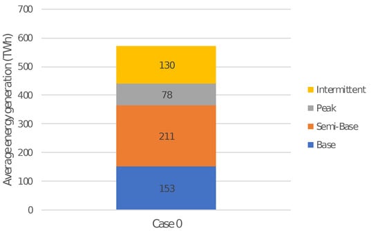
Figure 2.
Average generation breakdown for Case study 0.
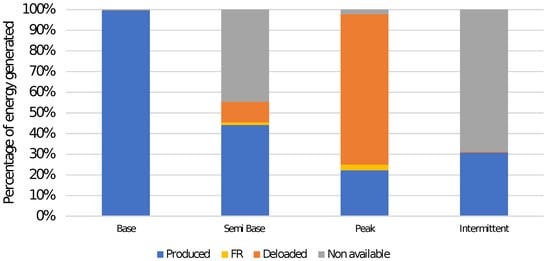
Figure 3.
Energy breakdown per technology type for Case study 0.
Note that, in this scenario, the CO2 emissions are significantly reduced to 21 Mt by comparison to 105 Mt in 2017 [47]. This value is still five times higher than the 4 Mt target set by Reference [47] in the UK pathways analysis, which could also be explained by the absence of Carbon Capture and Storage (CCS) in the assumptions surrounding the scenario investigated here.
4.1.2. Frequency Response
Figure 4 presents the average hourly frequency response requirement and the inertia of the system for Case study 0. The response is lower than the largest infeed loss (1800 MW), showing that the RoCoF and nadir constraints are easily respected with generation mix investigated. Only the steady-state constraint is binding, with the system being stable and exhibiting sufficient inertia.
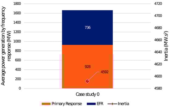
Figure 4.
Average hourly frequency response requirement and inertia for Case study 0.
In this case study, the PR is mainly provided by the semi-base units (CCGT and biomass) and by the interconnections: 549 MW from CCGT and 340 MW from interconnections. The rest is provided by biomass and PHS. Primary response and EFR have weekly and monthly seasonality (lower demand leads to lower inertia in the system and so higher response requirements), which, in Figure 5, shows the monthly average frequency response profile.
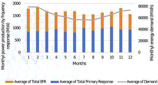
Figure 5.
Monthly frequency response profile for Case study 0.
Summer and winter daily profiles are presented Figure 6 for Case study 0. The demand curve directly depends on the consumption of residential heat (higher in winter), transport and industrial activities. For example, in December a peak in consumption is observed during the afternoon related to higher heating demand. The frequency response requirements are higher during summer, which is coherent given: lower consumption during summer which means less synchronous generators connected to the grid, since VRES output is high in these months, and, therefore, less inertia. The total requirements on the response (PR and EFR) are quite similar as a function of time, thanks to the variability of EFR. The EFR is injected into the network faster than the PR; hence, its beneficial impact is greater for the stability of the network, thus being the reason why the optimisation model prioritises EFR.
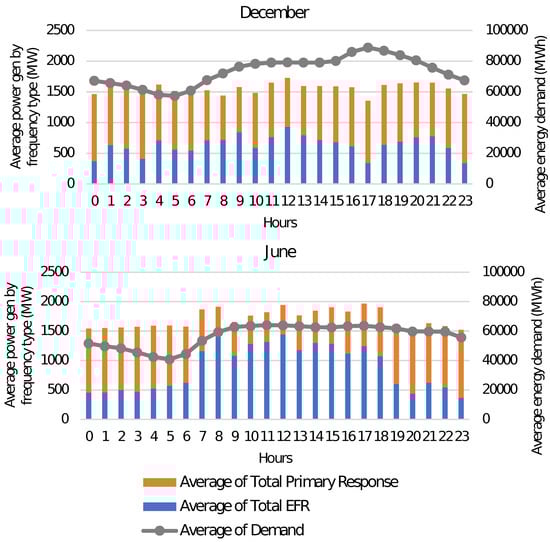
Figure 6.
Summer and winter daily frequency response profiles for Case study 0.
4.2. Case Study 1: Nuclear Flexibility
4.2.1. Energy and Carbon Dioxide Emissions
In this case, the objective is to assess the value of nuclear flexibility relative to Case 0 with consideration to higher nuclear flexibility under high VRES scenarios outlined in Case study 2 of this section. Figure 7 presents the generation breakdown for the case studies. There is almost no difference for the two cases even if nuclear flexibility is changed. The system is barely making use of the additional nuclear flexibility, as shown in Figure 8.
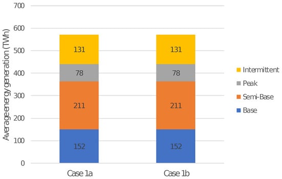
Figure 7.
Average generation breakdown for Case study 1.
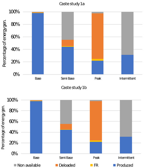
Figure 8.
Energy breakdown per technology type for Case study 1.
The similarities with the Case study 0 imply that this case study is not sufficient to reach the CO2 emissions reduction target (i.e., a different generation mix is required). The total CO2 emissions for Case 1a and Case 1b are also around 21 Mt each.
4.2.2. Frequency Response
With Figure 9, it is seen that changing the minimum stable factor of nuclear units from 55% to 20% does not have an impact on the frequency response requirements and total inertia, confirming that nuclear flexibility is not required for the system with this particular generation mix.
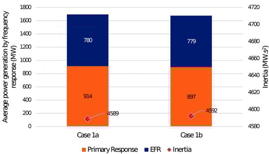
Figure 9.
Average hourly frequency response requirement and inertia for Case study 1.
4.3. Case Study 2: Semi-Base GAS Replaced by Nuclear
4.3.1. Energy and Carbon Dioxide Emissions
For Case 2a, all CCGT units are replaced by nuclear units, while, for Case 2b and 2c, all units are replaced by VRES. It is then more relevant to separate the analysis of Case 2a from the two other scenarios. Indeed, this comparison will allow for the assessment of the value of nuclear flexibility in a scenario without CCGT for semi-base production.
Figure 10 presents the generation breakdown for the three cases. Due to the low availability of wind at certain times of year, there are some hours pertaining to loss of load, which explains why the total energy generation is lower for cases 2b (32 TWh less) and 2c (with a difference of 33 TWh). More details will be provided in this section.
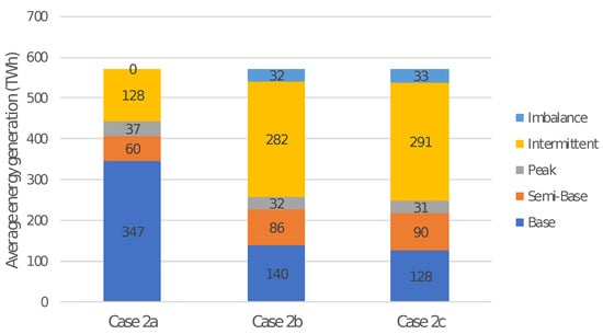
Figure 10.
Average generation breakdown for Case study 2.
As Figure 11 shows below, all cases without CCGT lead to higher de-load and, therefore, higher flexibility demand/usage for nuclear units than observed previously. When semi-base gas is replaced by nuclear, higher flexibility is observed for nuclear units, which are producing 69% of their potential on average (equivalent to 346 TWh) and 25% (equivalent to 126 TWh) is de-loaded. With respect to the online units, all the semi-base units are online and used at full capacity while a few peaking units are producing; however, the optimiser decides to shut down more peaking units and curtail more energy from VRES (10 TWh) relative to the base Case 0. The optimisation process decides to keep more than 95% of the nuclear units online even if this leads to more de-loading occurring in the nuclear units. Indeed, the model sees the value of inertia and opts for a system with greater inertia than that of the base case.
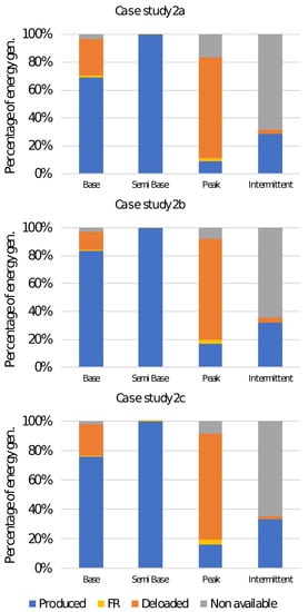
Figure 11.
Energy breakdown per technology type for Case study 2.
When gas is replaced by offshore wind (i.e., cases 2b and 2c), a greater demand for flexibility (due to a higher de-loading) is also observed for the nuclear fleet than in Case study 0 or Case study 1. It is important to note that with an MSF of 55%, the nuclear fleet is de-loading for 13% of its total capacity potential and by reducing the MSF from 55% to 21%, the de-loading is now about 20% of its total capacity. The difference in energy de-loaded by nuclear is equal to the VRES curtailed energy difference, which is around 14 TWh (see cases 2b and 2c in Figure 11).
An important point has been observed with the replacement of semi-base gas capacity by offshore wind capacity: the generation mix is not able to meet demand at all points in time. The lower availability of wind at certain times, leads to a high number of hours with significant loss of load. This situation is not acceptable in the UK power system and implies an insecure power system. More precisely, the system is imbalanced for 3286 h for a capacity of 17 GW on average and a total energy under supply of 32 TWh, which represents 6% of the annual demand. To tackle this imbalance issue, an increase of nuclear installed capacity would be beneficial for the system but would also change the system overall inertia and possibly the binding constraint. Moreover, removing semi-base gas units leads to a very large reduction of CO2 emissions, which is necessary to meet future emission goals. Only peaking units are emitting greenhouse gas emissions in these scenarios. For the Case 2a, with semi-base gas units replaced by nuclear, the total CO2 emissions are about 25 kt and when the units are replaced with VRES, the capacity factor of peak units is clearly increasing, so the CO2 emissions for a total of 422 kt in Case 2b and 426 kt in Case 2c. All those values respect the target outlined in the UK pathways report [47].
4.3.2. Frequency Response
As presented previously, in a scenario where all semi-base gas units are replaced by nuclear plants (Case study 2a), the system has sufficient inertia. Figure 12 shows that despite the huge increase in inertia associated with the high deployment level of nuclear (nuclear installed capacity increased by more than 50%), the frequency response requirements are similar. Indeed, having more nuclear units (with a higher inertia constant than gas units) is only increasing the overall inertia of a system that already exhibited sufficient inertia. That is why it is the steady-state constraint that is again binding the system in this case.
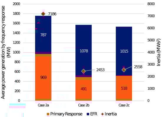
Figure 12.
Average hourly frequency response requirement and inertia for case study 2.
However, with a system where semi-base gas is replaced by VRES, the total inertia is significantly reduced on average by more than 40%. The average requirement of the total frequency response is slightly lower: 1569 MW for Case 2b and 1533 MW for Case 2c versus 1664 MW for the base case. However, the breakdown between PR and EFR is very different. Indeed, by comparing Figure 4 and Figure 12, the average PR requirements is decreased from 928 MW in Case 0 to 491 MW and 518 MW, respectively, for case 2b and 2c. On the contrary, the average EFR requirements are increased from 736 MW to 1078 MW and 1015 MW in case 2b and 2c, respectively. The model, therefore, decides to provide the power system with a faster frequency response using EFR. It appears that the nadir constraint is also a binding one by comparison to the Case 0. The optimisation model sees that it is more economically beneficial to quickly provide this frequency response using EFR rather than having a higher need of primary response. By comparing a 55% and 20% MSF, the average system inertia is slightly lower at 55%. Indeed, the number of nuclear units shutdown is higher in Case 2b than 2c as it will be presented in Section 4.4.
When the de-load is limited, the optimisation model sees the value of EFR rather than PR by increasing its requirement. It is indeed a key result of the sensitivity study: the increase of EFR capacity will decrease the need for primary reserve in the future and thereby increase the nuclear capacity factors. It is more valuable to tackle a post-fault frequency deviation quickly within 1 s rather than wait for a primary response in 10 s.
Note that with the given assumptions, on average, 1 GW of EFR provided by battery or interconnections and 0.5 GW of PR is enough to guarantee system security against post-fault frequency deviation. However, it is important to note the imbalance problem is still not solved with the given generation mix.
4.4. Impact of Flexibility Cases on Nuclear Operation
Table 3 presents an analysis of the number of shutdowns for the nuclear fleet. The results in Table 3 show that the optimisation model chooses to keep as many plants online as possible. This is because the value of the inertia provided by the nuclear units is generally recognised (even in the case where we replace all gas plants by nuclear, which makes nuclear plants operate part-loaded).
Table 3.
Annual nuclear shutdowns analysis.
The number of hours where at least one nuclear plant is offline is decreased when the MSF of nuclear is reduced. When semi-base gas plants are replaced by nuclear plants, one nuclear plant is not in use for at least 64% of the time. When it is replaced by offshore wind farms, one nuclear plant is not in use for 31% of the time if the MSF is at 55%. If the MSF is at 20%, the value for one nuclear plant not being used falls to 26% of the time. The optimisation model chose to have a higher flexibility on nuclear units and is willing to keep them online even if they are partly deloaded. The value of their inertia is recognised by the system, and the demand is then mainly met according to the merit order.
5. Discussion
Figure 13 shows a comparison of energy generation between the cases compared with the reference scenario (Case 0). In the reference scenario (Case 0), the system is not highly constrained by inertia reduction, and, due to the combined effect of: high demand; high nuclear installed capacity; and the high capacity of interconnectors, this results in a low/moderate need for flexibility.
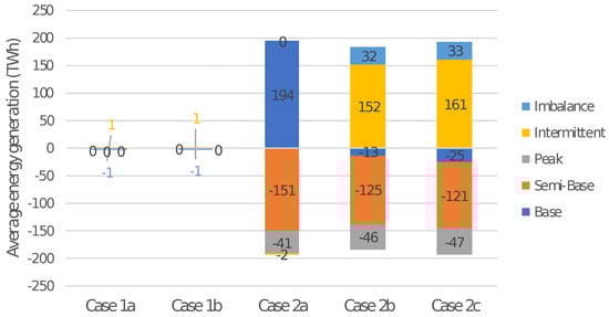
Figure 13.
Comparison of energy generation breakdown between cases relative to the base case (Case 0).
Figure 14 also shows the CO2 emissions between the scenarios, compared with the 2050 target outlined in Ref. [33]. As noted earlier, it is important to remember that in this investigation it has been assumed that CCS is not employed, therefore the displacement of gas plants with nuclear power plants or VRES (as per Case study 2) results in significant reductions in GHG emissions.
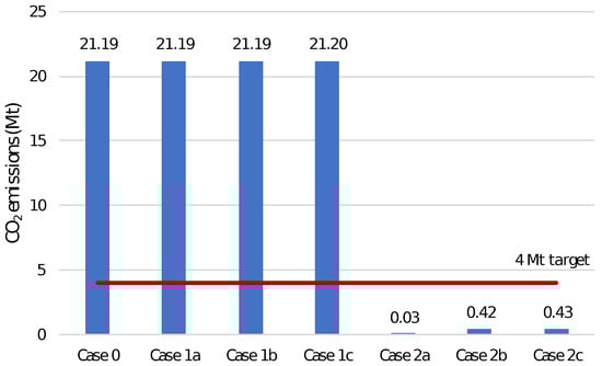
Figure 14.
Carbon dioxide emissions for each case study, compared with the 2050 target outlined in Ref. [33].
In Case study 1, which assesses the effect of increased flexibility in nuclear power plant operation relative to Case 0, this case study showed that this additional flexibility brings little additional value to the system. Having 55% or 20% nuclear MSF does not impact the system operation in this case. The steady-state constraint is the binding one. This condition does not depend on the dynamics of EFR or PR but in their quantities, which explains why the results are similar to Case 0.
In Case study 2, whereby gas plants were replaced by nuclear plants or offshore wind farms, the CO2 emissions reduce drastically: from 21 Mt in Case 0 and Cases 1 to 25 kt in case 2a and 422/426 kt in Cases 2b/2c (see Figure 14). When semi-base gas units are replaced by nuclear plants, the system once again meets the post-fault constraints and has sufficient inertia. A higher de-loading is observed in this case mainly due to the large amount of nuclear capacity that is not needed to meet the demand. When VRES is used to replace gas, the system inertia is significantly reduced (by more than 40%). The nadir constraint becomes then a binding one and the optimisation model sees the value of providing quickly EFR rather than PR. In addition to keeping the nuclear plants online and taking advantage of their inertia, the model is sensitive to the nuclear MSF. The higher the MSF is, the less flexible nuclear power plants are, which leads to more shutdowns. In this situation EFR, with its fast response, takes on the role of nuclear inertia, therefore reducing the primary reserve to a large extent. The potential increase of EFR in the future will lead to a decrease of PR and thereby reduce the requirement of flexibility from nuclear plants. Note that, in this generation mix, with CCGT being replaced by VRES, then, during low wind events the system is easily imbalanced (with around 6% of the annual demand is not met), and more generation capacity must be added. To tackle this imbalance issue, an increase in installed nuclear capacity would be beneficial for the system but would also change the overall inertia and possibly the binding constraint. Therefore, it is suggested that, in future work, an energy mix which finds a near optimal technology deployment based on high VRES and sufficient nuclear capacity, to find a scenario that simultaneously achieves low CO2 emissions, as well as acceptable post-fault system-level behaviour.
6. Conclusions
This study has been conducted to assess the value of increased flexible operation in Great Britain’s (GB’s) power system in the year 2050, while also assessing the extent of CO2 emission reductions. The general assumptions on the energy mix are taken from the European project EU SysFlex that has a coherent vision of the pan-European power systems and energy mixes. The total energy demand follows UK Pathways assumptions, which assumes a very high uptake of electric vehicles in the UK.
Considering the given set of assumptions, the main outcome of this study is that with a large proportion of nuclear and thermal assets (predominantly gas) the system inertia and the generation mix are sufficient to guarantee system security against post-fault frequency deviations. This is the case even in the presence of large EV deployment (12.6 million vehicles) with limited demand side management (smart charging only but without V2G capability). Sensitivities have been run to assess in Case 1 the value of flexibly operating nuclear power plants and Case 2 the feasibility of replacing all semi-base gas power plants by nuclear or off-shore wind technologies. The assessments focused on guaranteeing system security in the event of a loss of a generation unit.
Three distinct energy mixes are considered. The first scenario is a nominal case with significant components of nuclear (27% of average generation), thermal assets (37% of average generation and is dominated by gas) and VRES (23% of average generation), which was sufficient to guarantee system security but had high greenhouse gas emissions. The second scenario is a case with high nuclear (60% of average generation), moderate VRES penetration (20% of average generation) and low gas resulted in low emissions (25 kt) and a stable system. The final scenario relates to a case with high VRES (50% of average generation), low gas and moderate nuclear (20% of average generation), which resulted in low emissions (422 kt) but was imbalanced for 3286 h and led to around 6% of annual demand not being met.
In the sensitivity assessments, the value of keeping nuclear units online is recognised by the optimisation model, with a preference to keep nuclear units operating part-load and making use of their inherent inertia rather than shutting down nuclear units to deal with imbalances in load. The optimisation model illustrates how replacing Primary Response with Enhanced Frequency Response is very effective at mitigating the decrease in nuclear generation and allowing nuclear plants to operate at higher capacity factors. Finally, it is important to note: (1) these results are highly dependent on the evolution of different technologies and the level of electrification in different sectors; and (2) another uncertainty remains on the role of certain technologies that could provide ancillary services to support grid operation, including synchronous compensators for example.
Author Contributions
Conceptualization, A.B., A.P. and V.T.; methodology, A.B. and V.T.; software, A.B. and V.T.; validation, M.H.; formal analysis, A.P., B.M. and M.H.; investigation, A.B. and M.H.; resources, A.P.; data curation, M.H.; writing—original draft preparation, M.H.; writing—review and editing, A.P., B.M. and V.T.; visualization, M.H.; supervision, A.P.; project administration, A.P. and M.H.; funding acquisition, A.P. All authors have read and agreed to the published version of the manuscript.
Funding
This research was funded by the UK government’s Department for Business, Energy and Industrial Strategy, as part of the Energy Innovation Programme (Nuclear Facilities and Developing a Strategic Toolkit) grant number 13070002346.
Data Availability Statement
The data presented in this study are available on request from the corresponding author. The data are not publicly available due to some data sets being proprietary.
Acknowledgments
The authors would like to gratefully acknowledge input received from Thomas Bennett (NNL).
Conflicts of Interest
The authors declare no conflict of interest. The funders had no role in the design of the study; in the collection, analyses, or interpretation of data; in the writing of the manuscript, or in the decision to publish the results.
Abbreviations
The following abbreviations are used in this manuscript:
| CCGT | Combined Cycle Gas Turbine |
| CCS | Carbon Capture and Storage |
| CO2 | Carbon dioxide |
| EFR | Enhanced Frequency Response |
| EV | Electric Vehicle |
| FR | Frequency Response |
| GB | Great Britain |
| IR | Inertial Response |
| LP | Linear Programming |
| MILP | Mixed Integer Linear Programming |
| MSF | Minimum Stable Factor |
| OCGT | Open Cycle Gas Turbine |
| PHS | Pumped Hydro Storage |
| PR | Primary Response |
| PV | Photo Voltaic |
| RoCoF | Rate of Change of Frequency |
| UC | Unit Commitment |
| V2G | Vehicle to Grid |
| VRES | Variable Renewable Energy Sources |
References
- Johnson, S.C.; Rhodes, J.D.; Webber, M.E. Understanding the impact of non-synchronous wind and solar generation on grid stability and identifying mitigation pathways. Appl. Energy 2020, 262, 114492. [Google Scholar] [CrossRef]
- Chau, T.K.; Yu, S.S.; Fernando, T.L.; Iu, H.H.C.; Small, M. A novel control strategy of DFIG wind turbines in complex power systems for enhancement of primary frequency response and LFOD. IEEE Trans. Power Syst. 2017, 33, 1811–1823. [Google Scholar] [CrossRef]
- Greenwood, D.; Lim, K.Y.; Patsios, C.; Lyons, P.; Lim, Y.S.; Taylor, P. Frequency response services designed for energy storage. Appl. Energy 2017, 203, 115–127. [Google Scholar] [CrossRef]
- Boston, A.; Thomas, H.; Managing flexibility whilst decarbonising the GB electricity system. Energy Res. Partnersh. 2015. Available online: https://erpuk.org/wp-content/uploads/2015/12/1.-ERP-Boston.pdf (accessed on 1 December 2020).
- Peakman, A.; Merk, B.; Hesketh, K. The Potential of Pressurised Water Reactors to Provide Flexible Response in Future Electricity Grids. Energies 2020, 13, 941. [Google Scholar] [CrossRef]
- Kundur, P.; Balu, N.J.; Lauby, M.G. Power System Stability and Control; McGraw-Hill: New York, NY, USA, 1994; Volume 7. [Google Scholar]
- Trovato, V.; Bialecki, A.; Dallagi, A. Unit commitment with inertia-dependent and multispeed allocation of frequency response services. IEEE Trans. Power Syst. 2018, 34, 1537–1548. [Google Scholar] [CrossRef]
- Tan, Y.; Muttaqi, K.M.; Ciufo, P.; Meegahapola, L. Enhanced frequency response strategy for a PMSG-based wind energy conversion system using ultracapacitor in remote area power supply systems. IEEE Trans. Ind. Appl. 2017, 53, 549–558. [Google Scholar] [CrossRef]
- Díaz-González, F.; Hau, M.; Sumper, A.; Gomis-Bellmunt, O. Participation of wind power plants in system frequency control: Review of grid code requirements and control methods. Renew. Sustain. Energy Rev. 2014, 34, 551–564. [Google Scholar] [CrossRef]
- Li, P.; Hu, W.; Hu, R.; Huang, Q.; Yao, J.; Chen, Z. Strategy for wind power plant contribution to frequency control under variable wind speed. Renew. Energy 2019, 130, 1226–1236. [Google Scholar] [CrossRef]
- De Rijcke, S.; Tielens, P.; Rawn, B.; Van Hertem, D.; Driesen, J. Trading energy yield for frequency regulation: Optimal control of kinetic energy in wind farms. IEEE Trans. Power Syst. 2014, 30, 2469–2478. [Google Scholar] [CrossRef]
- NG. Frequency Response Technical Sub-Group Report; Technical Report; 2011. Available online: https://www.nationalgrideso.com/document/25546/download (accessed on 4 January 2021).
- Kheshti, M.; Ding, L.; Bao, W.; Yin, M.; Wu, Q.; Terzija, V. Toward intelligent inertial frequency participation of wind farms for the grid frequency control. IEEE Trans. Ind. Inform. 2019, 16, 6772–6786. [Google Scholar] [CrossRef]
- Tsormpatzoudis, V.; Forsyth, A.J.; Todd, R. Rapid Evaluation of Battery System Rating For Frequency Response Operation. In Proceedings of the 2019 IEEE Milan PowerTech, Milan, Italy, 23–27 June 2019; pp. 1–6. [Google Scholar]
- Trovato, V.; Sanz, I.M.; Chaudhuri, B.; Strbac, G. Advanced control of thermostatic loads for rapid frequency response in Great Britain. IEEE Trans. Power Syst. 2016, 32, 2106–2117. [Google Scholar] [CrossRef]
- HM Government. 2050 Pathways Analysis; Technical Report; Department of Energy and Climate Change: 2010. Available online: https://assets.publishing.service.gov.uk/government/uploads/system/uploads/attachment_data/file/42562/216-2050-pathways-analysis-report.pdf (accessed on 1 December 2020).
- Pina, A.; Silva, C.A.; Ferrão, P. High-resolution modeling framework for planning electricity systems with high penetration of renewables. Appl. Energy 2013, 112, 215–223. [Google Scholar] [CrossRef]
- Price, J.; Zeyringer, M.; Konadu, D.; Mourão, Z.S.; Moore, A.; Sharp, E. Low carbon electricity systems for Great Britain in 2050: An energy-land-water perspective. Appl. Energy 2018, 228, 928–941. [Google Scholar] [CrossRef]
- Zeyringer, M.; Price, J.; Fais, B.; Li, P.H.; Sharp, E. Designing low-carbon power systems for Great Britain in 2050 that are robust to the spatiotemporal and inter-annual variability of weather. Nat. Energy 2018, 3, 395–403. [Google Scholar] [CrossRef]
- Pfenninger, S.; Keirstead, J. Renewables, nuclear, or fossil fuels? Scenarios for Great Britain’s power system considering costs, emissions and energy security. Appl. Energy 2015, 152, 83–93. [Google Scholar] [CrossRef]
- Ekins, P.; Keppo, I.; Skea, J.; Strachan, N.; Usher, W.; Anandarajah, G. The UK Energy System in 2050: Comparing Low-Carbon, Resilient Scenarios. 2013. Available online: http://www.ukerc.ac.uk/support/tiki-download_file.php?fileId=2976 (accessed on 1 December 2020).
- NG. Future Energy Scenarios 2018. National Grid 2018. Available online: https://www.nationalgrideso.com/sites/eso/files/documents/fes-2018-faqs-for-website-v30.pdf (accessed on 4 January 2021).
- Chávez, H.; Baldick, R.; Sharma, S. Governor rate-constrained OPF for primary frequency control adequacy. IEEE Trans. Power Syst. 2014, 3, 1473–1480. [Google Scholar] [CrossRef]
- Ahmadi, H.; Ghasemi, H. Security-constrained unit commitment with linearized system frequency limit constraints. IEEE Trans. Power Syst. 2014, 29, 1536–1545. [Google Scholar] [CrossRef]
- Teng, F.; Trovato, V.; Strbac, G. Stochastic scheduling with inertia-dependent fast frequency response requirements. IEEE Trans. Power Syst. 2015, 31, 1557–1566. [Google Scholar] [CrossRef]
- Cardozo, C.; Van Ackooij, W.; Capely, L. Cutting plane approaches for frequency constrained economic dispatch problems. Electr. Power Syst. Res. 2018, 156, 54–63. [Google Scholar] [CrossRef]
- Trovato, V.; Teng, F.; Strbac, G. Role and benefits of flexible thermostatically controlled loads in future low-carbon systems. IEEE Trans. Smart Grid 2017, 9, 5067–5079. [Google Scholar] [CrossRef]
- Badesa, L.; Teng, F.; Strbac, G. Simultaneous scheduling of multiple frequency services in stochastic unit commitment. IEEE Trans. Power Syst. 2019, 34, 3858–3868. [Google Scholar] [CrossRef]
- Chu, Z.; Markovic, U.; Hug, G.; Teng, F. Towards optimal system scheduling with synthetic inertia provision from wind turbines. IEEE Trans. Power Syst. 2020, 35, 4056–4066. [Google Scholar] [CrossRef]
- Paturet, M.; Markovic, U.; Delikaraoglou, S.; Vrettos, E.; Aristidou, P.; Hug, G. Stochastic unit commitment in low-inertia grids. IEEE Trans. Power Syst. 2020, 35, 3448–3458. [Google Scholar] [CrossRef]
- Rahmani, M.; Hosseinian, S.H.; Abedi, M. Stochastic two-stage reliability-based Security Constrained Unit Commitment in smart grid environment. Sustain. Energy Grids Netw. 2020, 22, 100348. [Google Scholar] [CrossRef]
- EU-SysFlex. EU-SysFlex Scenarions and Network Sensitivities; Technical Report; EU-SysFlex: 2018. Available online: http://eu-sysflex.com/wp-content/uploads/2018/12/D2.2_EU-SysFlex_Scenarios_and_Network_Sensitivities_v1.pdf (accessed on 1 December 2020).
- BEIS. The Clean Growth Strategy: Leading the Way to a Low Carbon Future. 2018. Available online: https://assets.publishing.service.gov.uk/government/uploads/system/uploads/attachment_data/file/700496/clean-growth-strategy-correction-april-2018.pdf (accessed on 1 December 2020).
- ESC. Preparing UK Electricity Networks for Electric Vehicles Report. 2018. Available online: https://es.catapult.org.uk/reports/preparing-uk-electricity-networks-for-electric-vehicles/ (accessed on 1 December 2020).
- Faunce, T.A.; Prest, J.; Su, D.; Hearne, S.J.; Iacopi, F. On-grid batteries for large-scale energy storage: Challenges and opportunities for policy and technology. MRS Energy Sustain. 2018, 5, E11. [Google Scholar] [CrossRef]
- Li, N.; Hedman, K.W. Evaluation of the adjustable-speed pumped hydro storage in systems with renewable resources. In Proceedings of the 2016 IEEE/PES Transmission and Distribution Conference and Exposition (T&D), Dallas, TX, USA, 3–5 May 2016; pp. 1–5. [Google Scholar]
- Wilson, P.D. The Nuclear Fuel Cycle: From Ore to Wastes; Oxford University Press: Oxford, UK, 1996. [Google Scholar]
- Lee, W.E.; Ojovan, M.I.; Jantzen, C.M. Radioactive Waste Management and Contaminated Site Clean-up: Processes, Technologies and International Experience; Elsevier: Amsterdam, The Netherlands, 2013. [Google Scholar]
- Peakman, A.; Gregg, R. The Fuel Cycle Implications of Nuclear Process Heat. Energies 2020, 13, 6073. [Google Scholar] [CrossRef]
- NG. Grid Code—Connection Condition. 2018. Available online: https://www.nationalgrid.com/sites/default/files/documents/8589935284-Connection%20Conditions.pdf (accessed on 4 January 2021).
- Spallarossa, C.; Merlin, M.; Green, T. Augmented inertial response of multi-level converters using internal energy storage. In Proceedings of the 2016 IEEE International Energy Conference (ENERGYCON), Leuven, Belgium, 4–8 April 2016; pp. 1–6. [Google Scholar]
- Gundogdu, B.; Nejad, S.; Gladwin, D.T.; Stone, D.A. A battery energy management strategy for UK enhanced frequency response. In Proceedings of the 2017 IEEE 26th International Symposium on Industrial Electronics (ISIE), Edinburgh, UK, 19–21 June 2017; pp. 26–31. [Google Scholar]
- Spillett, D. Frequency changes during large disturbances and their impact on the total system. Natl. Grid Warwick U. K. Tech. Rep. 2013. Available online: https://www.nationalgrideso.com/document/10821/download (accessed on 4 January 2021).
- Zhang, L.; Capuder, T.; Mancarella, P. Unified unit commitment formulation and fast multi-service LP model for flexibility evaluation in sustainable power systems. IEEE Trans. Sustain. Energy 2015, 7, 658–671. [Google Scholar] [CrossRef]
- Chen, H.; Liu, M.; Cheng, Y.; Lin, S. Modeling of Unit Commitment with AC Power Flow Constraints Through Semi-Continuous Variables. IEEE Access 2019, 7, 52015–52023. [Google Scholar] [CrossRef]
- Trovato, V.; Mazza, A.; Chicco, G. Flexible operation of low-inertia power systems connected via high voltage direct current interconnectors. Electr. Power Syst. Res. 2020, 192, 106911. [Google Scholar] [CrossRef]
- BEIS. Report Greenhouse Gas Emissions, Provisional Figures Statistical Release: National Statistics; 2017. Available online: https://assets.publishing.service.gov.uk/government/uploads/system/uploads/attachment_data/file/695930/2017_Provisional_Emissions_statistics_2.pdf (accessed on 4 January 2021).
Publisher’s Note: MDPI stays neutral with regard to jurisdictional claims in published maps and institutional affiliations. |
© 2021 by the authors. Licensee MDPI, Basel, Switzerland. This article is an open access article distributed under the terms and conditions of the Creative Commons Attribution (CC BY) license (http://creativecommons.org/licenses/by/4.0/).