Model-Based Analysis of Flow Separation Control in a Curved Diffuser by a Vibration Wall

Abstract

Vibration wall control is an important active flow control technique studied by many researchers. Although current researches have shown that the control performance is greatly affected by the frequency and amplitude of the vibration wall, the mechanism hiding behind the phenomena is still not clear, due to the complex interaction between the vibration wall and flow separation. To reveal the control mechanism of vibration walls, we propose a simplified model to help us understand the interaction between the forced excitation (from the vibration wall) and self-excitation (from flow instability). The simplified model can explain vibration wall flow control behaviors obtained by numerical simulation, which show that the control performance will be optimized at a certain reduced vibration frequency or amplitude. Also, it is shown by the analysis of maximal Lyapunov exponents that the vibration wall is able to change the flow field from a disordered one into an ordered one. Consistent with these phenomena and bringing more physical insight, the simplified model implies that the tuned vibration frequency and amplitude will lock in the unsteady flow separation, promote momentum transfer from the main stream to the separation zone, and make the flow field more orderly and less chaotic, resulting in a reduction of flow loss.

1. Introduction

Flow separation is generally accepted to be the breakaway or detachment of fluid from a solid surface [1]. It often leads to liftor total pressure efficiency decreases of wings or diffusers. Thus, researchers from all over the world are seeking the way to avoid or suppress flow separation. Furthermore, it is widely accepted that unsteady flow control techniques need less energy input than steady ones to achieve the same control performance [2]. Typical existing active control methods include acoustic excitation [3], synthetic jet [4], pulsed jet [5], plasma actuation [6], and vibration wall [7]. Among them, vibration wall is becoming popular because it has a simple structure and does not change the surface shape when not working (better than most passive flow control methods which may cause additional losses under an off-design point). Regarding the vibration wall, Wu [7] studied the effect of wall vibration on flow separation and raised the concept of “streaming effect” which is used to evaluate the control performance. Sinha [8] introduced the active flexible wall (AFW) and showed a that proper vibration frequency can optimize the velocity profile of the boundary layer and delay flow separation. Yang [9] studies the effect of wall vibration frequency on a low-pressure turbine cascade. It is found that a certain frequency range will lead to a minimum cascade loss and then low-energy fluid is confined near the suction surface by energy exchange between the free flow and near-wall flow. Moreover, Kang [10] used wall vibration to control flow separation on an airfoil and also found a certain frequency range of lift enhancement accompanied by frequency synchronization.

Although the previous studies have shown the relationship between the parameters of vibration walls and control performance, the mechanism that how these parameters function is still not clear. In some other unsteady flow control methods, detailed experimental and numerical results imply and reveal some mechanisms hidden behind the unique phenomena, which vibration wall control may share. For example, in pulsed jet flow control, when the frequency of the pulsed jet is equal to the dominant frequency of the shedding vortex, the control performance reaches its peak [2,11]. This kind of frequency-dependent phenomenon also exists in Yang and Kang’s work [9,10] as mentioned before. As it is known, tuned external excitation can stimulate large-scale coherent structures in separated flows via flow instability [12]. Also, some works indicate that effective excitation tends to change a chaotic flow field into a relatively ordered one [11]. This implies the interaction between external periodic excitation and unsteady flow separation may fall in the category of chaos control, which may also apply to vibration wall control.

With the known clues discussed before, we are thinking of a way to analyze the mechanism of vibration wall control in a clearer way. It is accepted that complex phenomenon doesn’t always mean complex mechanisms, and the misunderstanding often occurs because of taking a part for the whole. Simplified models are very helpful for us to understand the simple mechanism hidden behind the complex phenomena. For example, in computational fluid dynamics, some simple equations (toy models) are studied in priority and compatible schemes can be developed to solve complex formula then. Based on the same train of thought, in this paper, we employ a simplified model to help us understand the mechanism and phenomena in vibration wall control. Because flow instability is the basis of unsteady flow control, the flow instability theory is of great importance as references for vibration wall control. The flow instability theory includes two typical models, the O-S (Orr–Sommerfeld) equation and the S-L (Stuart–Landau) equation. The O-S equation [13] is based on the linear perturbation theory and used to describe flow stability in parallel flows. Although the linear perturbation theory is relatively mature and agrees with many experimental results, it only applies to the initial phase of flow instability, after which the nonlinear effect plays the leading role. Then, as a weak nonlinear flow instability theory, the S-L equation [14] can be used to deal with flow stability problems with weak nonlinearity. However, all these simplified models for linear or weak nonlinear applications, are not suitable for describing unsteady flow control with strong nonlinearity, especially with chaos. Therefore, in this paper, we introduce a simplified model to describe the interaction between the forced excitation (from vibration wall) and self-excitation (from flow instability), and analyze the phenomena and mechanism of vibration wall flow control based on this model.

2. A Nonlinear Simplified Model for Flow Separation Control by a Vibration Wall

In this section, we establish a nonlinear simplified model to describe the effect of a vibration wall on unsteady flow separation. Considering the 2D incompressible N-S Equation:

$$\frac{d\overrightarrow{V}}{dt}=-\frac{1}{\rho }\nabla p+\nu {\nabla }^2\overrightarrow{V}$$

(1)

To reduce the order of this formula, only y-direction (basically perpendicular to the main flow direction) movement is considered. Therefore, Equation (1) is restated as:

$$\frac{{\partial }^{2}y(\xi ,\eta ,t)}{\partial t^2}=-\frac{1}{\rho }\frac{\partial }{\partial y}p(x,y,t)+\nu (\frac{{\partial }^2}{\partial x^2}+\frac{{\partial }^2}{\partial y^2})V_y(x,y,t)$$

(2)

where $\xi$, $\eta$ are Lagrange variables used to distinguish the fluid particles. For a particular fluid particle denoted by ${\xi }_0$ and ${\eta }_0$:

$$\begin{array}{l}\frac{d^{2}y({\xi }_0,{\eta }_0,t)}{d{t}^2}=\left[-\frac{1}{\rho }\frac{\partial }{\partial y}p(x,y,t)+\nu (\frac{{\partial }^2}{\partial x^2}+\frac{{\partial }^2}{\partial y^2})V_y(x,y,t)\right]\left|{}_{x=x({\xi }_0,{\eta }_0,t),y=y({\xi }_0,{\eta }_0,t)}\right.\\ \approx \left[-\frac{1}{\rho }\overline{\frac{\partial }{\partial y}p(x,y,t)}+\nu \overline{(\frac{{\partial }^2}{\partial x^2}+\frac{{\partial }^2}{\partial y^2})V_y(x,y,t)}+f(t)\right]\left|{}_{x=x({\xi }_0,{\eta }_0,t),y=y({\xi }_0,{\eta }_0,t)}\right.\end{array}$$

(3)

where $\overline{a}$ means the time-averaged function $a$. In Equation (3), $-\frac{1}{\rho }\overline{\frac{\partial }{\partial y}p(x,y,t)}$ is a time-averaged pressure gradient term, $\nu \overline{(\frac{{\partial }^2}{\partial x^2}+\frac{{\partial }^2}{\partial y^2})V_y(x,y,t)}$ is a time-averaged dissipation term, and $f(t)$ is a time-dependent term defined as:

$$f(t)=-\frac{1}{\rho }\left[\frac{\partial }{\partial y}p(x,y,t)-\overline{\frac{\partial }{\partial y}p(x,y,t)}\right]+\nu \left[(\frac{{\partial }^2}{\partial x^2}+\frac{{\partial }^2}{\partial y^2})V_y(x,y,t)-\overline{(\frac{{\partial }^2}{\partial x^2}+\frac{{\partial }^2}{\partial y^2})V_y(x,y,t)}\right]$$

(4)

and it is easy to deduce that $\overline{f(t)}=0$. So, in the following passage, we aim at modeling these three terms (the time-averaged pressure gradient term, the time-averaged dissipation term and the time-dependent term), separately.

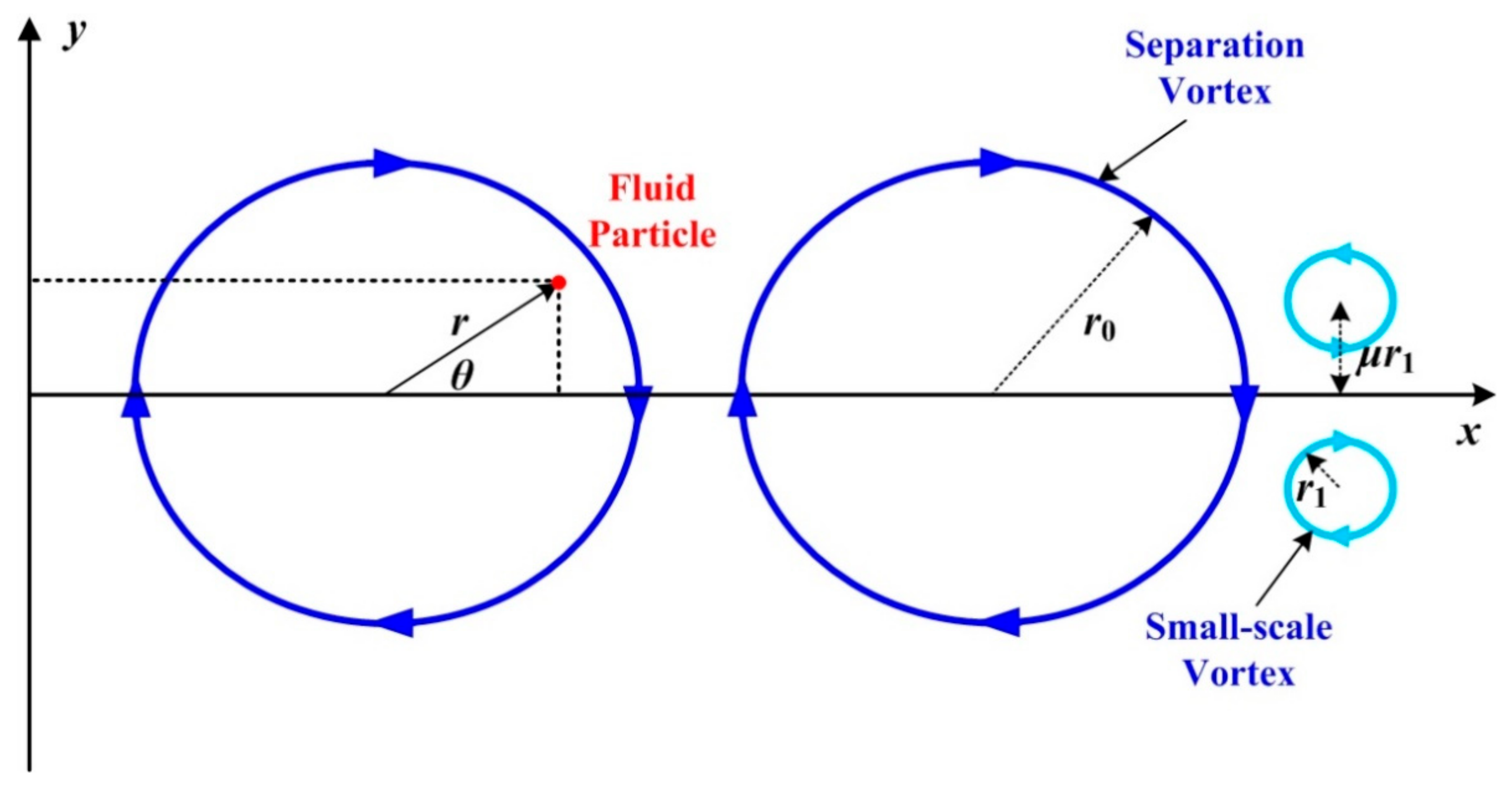
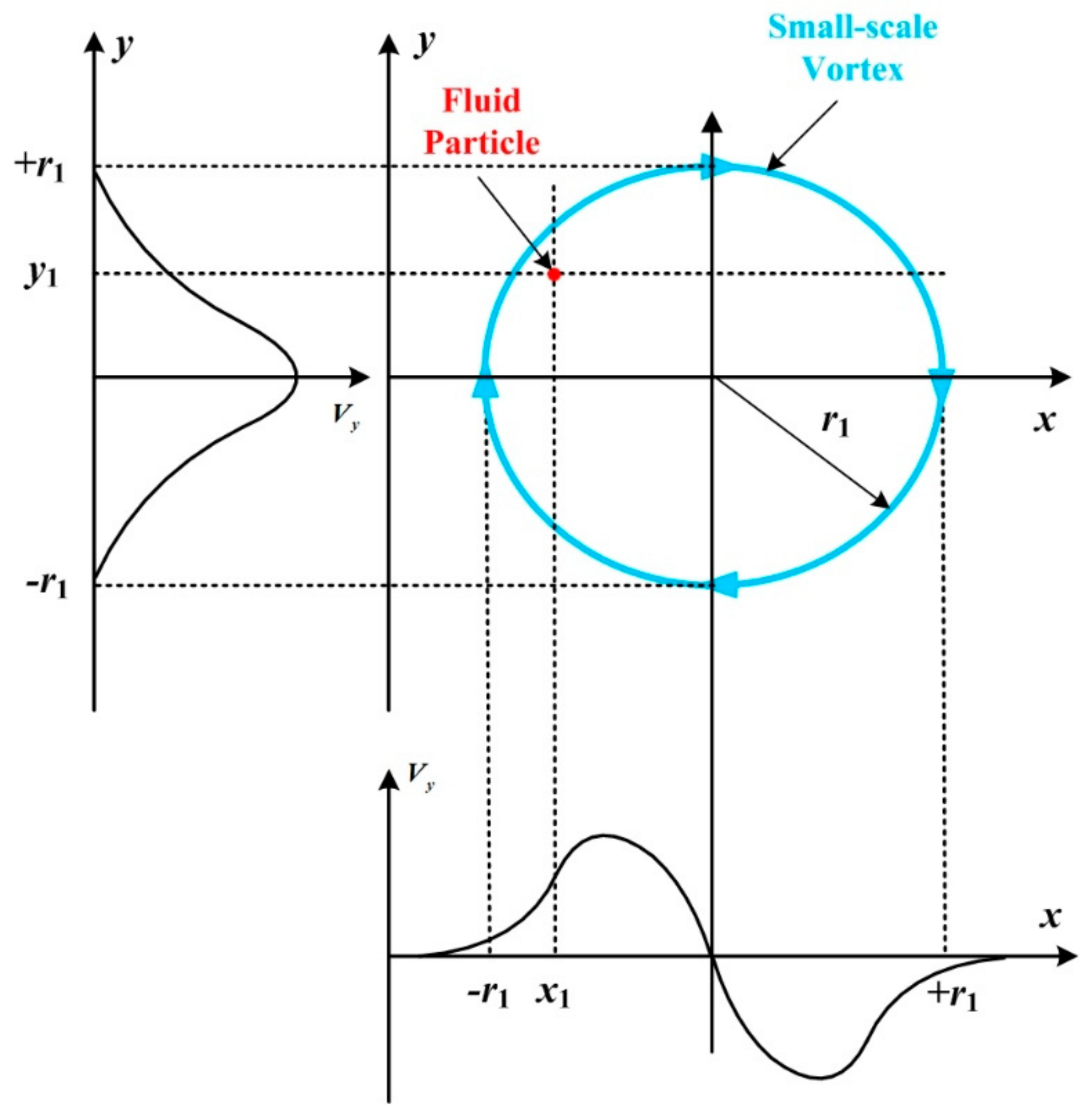
2.1. Time-Averaged Pressure Gradient Based on the Concentrated Vortex Model

In this section, we build a simplified model for the time-averaged pressure gradient term $-\frac{1}{\rho }\overline{\frac{\partial }{\partial y}p(x,y,t)}$ in Equation (3) based on a concentrated vortex model. When the separation vortex reaches its saturation stage (when its scale and strength do not change a lot), it can be modeled as a vortex row consisting of identical concentrated vortices, as shown in Figure 1. In addition, we make the x-axis pass through the vortex cores of separation vortices and assume all small-scale vortices are symmetric with respect to the x-axis. It is known the pressure gradient in a concentrated vortex is:

$$\frac{1}{\rho }\frac{\partial p}{\partial r}=\frac{V_{\theta }{}^2}{r}$$

(5)

where $V_{\theta }{}^{}$ is the circumferential velocity. Here, we introduce Oseen vortex model [15], which is a kind of symmetry isolated vortex and an accurate solution of the incompressible N-S equation. The Oseen vortex is a circular vortex and it is more physical than other vortex models such as point vortex, rigid body vortex and Rankine vortex. Its circumferential velocity distribution can be described as:

$$V_{\theta }=\frac{{\mathrm{\Gamma }}_0}{2\pi r}(1-e^{-r^2/(4\nu t)})$$

(6)

where, ${\mathrm{\Gamma }}_0$ is vortex strength. If we define the vortex core radius as: $r_0=2\sqrt{\nu t}$. Then, on one hand, when $r/r_0\ll 1$, $V_{\theta }\approx {\mathrm{\Gamma }}_{0}r/(8\pi \nu t)$, so the velocity distribution in the vortex core zone is similar to that of a rigid body vortex. On the other hand, when $r/r_0\gg 1$, $V_{\theta }\approx {\mathrm{\Gamma }}_0/(2\pi r)$, the velocity distribution outside the vortex core zone is similar to that of a point vortex.

We consider a situation that a fluid particle is dominated by a separation vortex (near the core of an Oseen vortex). The y-direction pressure gradient is:

$$-\frac{1}{\rho }\frac{\partial p}{\partial y}=-\frac{1}{\rho }\frac{\partial p}{\partial r}\sin \theta =-\frac{{\mathrm{\Gamma }}_0^2}{4{\mathsf{\pi }}^2{r}^3}{(1-{\mathrm{e}}^{-r^2/r_0^2})}^2\sin \theta$$

(7)

If $\theta \approx \mathsf{\pi }/2$ and $y\ll r_0$, then $r\approx y$ and $\sin \theta \approx 1$. According to the Taylor expansion approximation that $e^x\approx 1+x+x^2/2$, it can be deduced that:

$$-\frac{1}{\rho }\frac{\partial p}{\partial y}\approx \frac{{\mathrm{\Gamma }}_0^2}{4{\mathsf{\pi }}^2{r}_0^4}(-y+\frac{y^3}{r_0^2})$$

(8)

Moreover, we consider a situation that a fluid particle is affected by two symmetrical small-scale vortices (two Oseen vortices with the radius $r_1$) at a distance of $2\mu r_1$ (as shown in Figure 1). If the fluid particle is near the symmetric line, the y-direction pressure gradient is considered approximately as the superposition of two isolated Oseen vortices, stated as:

$$\begin{array}{l}-\frac{1}{\rho }\frac{\partial p}{\partial y}\approx -\frac{{\mathrm{\Gamma }}_0^2}{4{\mathsf{\pi }}^2{r}_1^3}[\frac{{(1-{\mathrm{e}}^{-{(y/r_1-\mu )}^2})}^2}{{(y/r_1-\mu )}^3}+\frac{{(1-{\mathrm{e}}^{-{(y/r_1+\mu )}^2})}^2}{{(y/r_1+\mu )}^3}]\\ \approx \frac{{\mathrm{\Gamma }}_0^2}{4{\mathsf{\pi }}^2{r}_1^4}(k_{1}y+k_3\frac{y^3}{r_1^2})\end{array}$$

(9)

where $k_1$ and $k_3$ are coefficients depending on $\mu$. Then, Equation (8) can be regarded as a particular case of Equation (9) when $\mu =0$ and $r_1=r_0$. So, when $\mu$ changes, so are $k_1$ and $k_3$ (Some cases are listed in

Table 1. $k_1$ & $k_3$ versus $\mu$.

$\mathit{\mu }$	${\mathit{k}}_1$	${\mathit{k}}_3$
0	−1	+1
0.5	−0.82	−0.02
1	+0.54	−1.01
2	+0.33	+0.1

).

When we track a fluid particle, $k_1$ and $k_3$ are not fixed (both their values and signs are time-dependent), an approximate expression of pressure gradient is shown as:

$$-\frac{1}{\rho }\frac{\partial }{\partial y}p(x,y,t)\approx \frac{{\mathrm{\Gamma }}_0^2(t)}{4{\mathsf{\pi }}^2{r}_0^4(t)}(k_1(t)y+\frac{k_3(t)}{r_0^2(t)}{y}^3)$$

(10)

Furthermore, the time-averaged pressure gradient has the expression:

$$\begin{array}{l}-\frac{1}{\rho }\overline{\frac{\partial }{\partial y}p(x,y,t)}\left|{}_{x=x({\xi }_0,{\eta }_0,t),y=y({\xi }_0,{\eta }_0,t)}\right.\\ \approx \frac{1}{4{\mathsf{\pi }}^2}\overline{k_1(t){\mathrm{\Gamma }}_0^2(t)r_0^{-4}(t)}y({\xi }_0,{\eta }_0,t)+\frac{1}{4{\mathsf{\pi }}^2}\overline{k_3(t){\mathrm{\Gamma }}_0^2(t)r_0^{-6}(t)}{y}^3({\xi }_0,{\eta }_0,t)\\ =-ay-c{y}^3\end{array}$$

(11)

So, in Equation (3), if we only take the pressure gradient into account, then:

$$\frac{{\mathrm{d}}^{2}y}{\mathrm{d}{t}^2}=-\frac{1}{\rho }\overline{\frac{\partial }{\partial y}p(x,y,t)}\approx -ay-c{y}^3$$

(12)

This is a typical conservative Duffing equation [16]. When the signs of $a$ and $c$ change, so is the type of the Duffing equation and its nonlinear characteristics (See

Table 2. Types of the Duffing equation (data from Ref. [16]).

$\mathbf{sgn}(\mathit{a})$	$\mathbf{sgn}(\mathit{c})$	Types of the Duffing Equation
+	−	softening nonlinearity
+	+	hardening nonlinearity
−	+	Negative linear positive cubic stiffness nonlinearity
−	−	Negative linear negative cubic stiffness nonlinearity

).

So, according to Equations (11) and (12), the strength, scale and formation of separation vortices and small-scale vortices affect the time-averaged pressure gradient and the type of the Duffing equation. Furthermore, different types of the Duffing equation present totally different characteristics. For example, the Duffing equation with negative linear positive cubic stiffness nonlinearity has chaotic solutions. This type is focused on in this paper because chaos is a crucial feature in unsteady flow separation.

2.2. Time-Averaged Dissipation Term

In this section, we model the time-averaged dissipation term $\nu \overline{(\frac{{\partial }^2}{\partial x^2}+\frac{{\partial }^2}{\partial y^2})V_y(x,y,t)}$ in Equation (3). We know that small-scale vortices rather than large-scale vortices contribute to the dissipation of mechanical energy mostly in an unsteady flow field. So, we first inspect the dissipation in a small-scale vortex. Using the central difference scheme, we know that:

$$\frac{{\partial }^2}{\partial x^2}{V}_y(x,y,t)=\underset{r_1\to 0}{\lim }\frac{V_y(x+2r_1,y,t)+V_y(x-2r_1,y,t)-2V_y(x,y,t)}{4r_1^2}$$

(13)

where $r_1$ is the vortex core radius of a small-scale vortex. As shown in Figure 2, for a small-scale vortex, its y-direction velocity ($V_y=0$ for the mainstream) decays rapidly outside its vortex core. So, $V_y(x+2r_1,y,t)\approx 0$ and $V_y(x-2r_1,y,t)\approx 0$. Also, for a small-scale vortex, $r_1$ is very small and thus:

$$\frac{{\partial }^2}{\partial x^2}{V}_y(x,y,t)\approx \frac{-V_y(x,y,t)}{2r_1^2}$$

(14)

Using the same technique for $\frac{{\partial }^2}{\partial y^2}{V}_y(x,y,t)$, we can deduce that:

$$(\frac{{\partial }^2}{\partial x^2}+\frac{{\partial }^2}{\partial y^2})V_y(x,y,t)\approx \frac{-V_y(x,y,t)}{r_1^2}$$

(15)

So:

$$\begin{array}{l}\nu (\frac{{\partial }^2}{\partial x^2}+\frac{{\partial }^2}{\partial y^2})V_y(x,y,t)\left|{}_{x=x({\xi }_0,{\eta }_0,t),y=y({\xi }_0,{\eta }_0,t)}\right.\approx -\nu \frac{V_y(x,y,t)}{r_1^2(t)}\left|{}_{x=x({\xi }_0,{\eta }_0,t),y=y({\xi }_0,{\eta }_0,t)}\right.\\ =-\nu \frac{V_y({\xi }_0,{\eta }_0,t)}{r_1^2(t)}=-\nu \frac{1}{r_1^2(t)}\frac{dy}{dt}\end{array}$$

(16)

The right part of this equation is a time-dependent damping term with a time-dependent damping coefficient $-\nu r_1^{-2}(t)$, where $r_1^{}(t)$ describes the radius of small-scale vortices a fluid particle encounters. Because the radius of the large-scale separation vortex is $r_0^{}$ ($r_0^{}>r_1^{}(t)$), the time-averaged dissipation term scaled by $r_0^{}$ can be restated as:

$$\nu \overline{(\frac{{\partial }^2}{\partial x^2}+\frac{{\partial }^2}{\partial y^2})V_y(x,y,t)}\left|{}_{x=x({\xi }_0,{\eta }_0,t),y=y({\xi }_0,{\eta }_0,t)}\right.=-\frac{\nu +{\nu }_T}{r_0^2}\frac{dy}{dt}=-e\frac{dy}{dt}$$

(17)

where, ${\nu }_T$ is the added eddy viscosity due to small-scale vortices during the scaling and time-averaged procedure, and the damping term is then a time-independent constant (the damping coefficient is $e$), which is much easier for subsequent treatment. Now, we have completed the modeling of the time-averaged dissipation term in Equation (3).

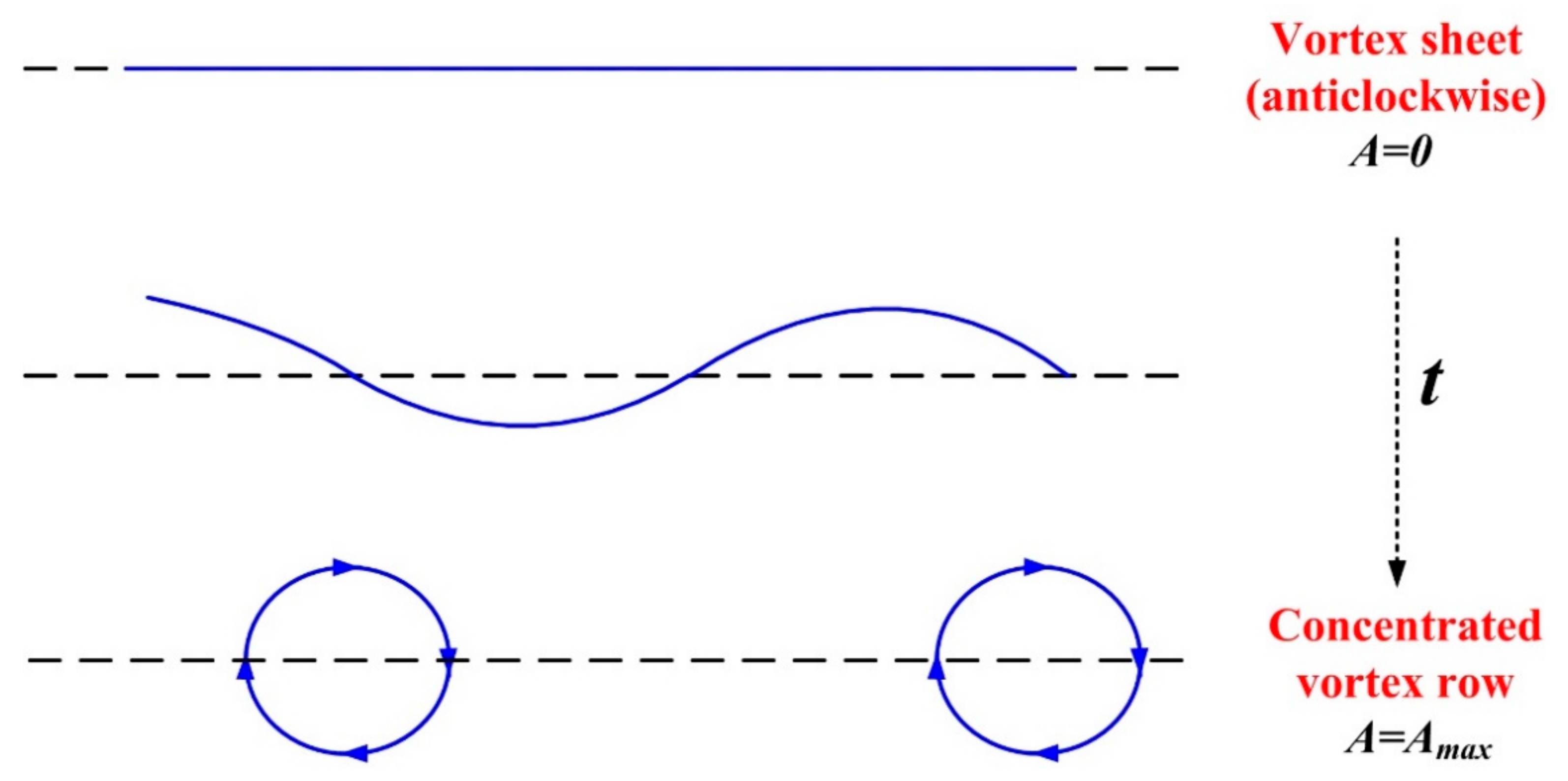
2.3. Time-Dependent Term Based on the Self-Excitation and External Excitation Model

In this section, we aim to model the time-dependent term $f(t)$. The modeling based on its complex definition (Equation (4)) is very difficult, however, another way for modeling is based on its physical meaning. We know the unsteadiness in unsteady flow separation control come from two sources. One is the self-excitation due to internal flow instability which is responsible for the large-scale vortical structures of flow separation, and another is the external periodic excitation produced by unsteady flow control.

Figure 3 shows the evolutionary process of a vortex sheet rolling into a concentrated vortex row due to K-H instability, which is interpreted by Batchelor [15]. If we follow a fluid particle, it will experience vortex induced motion, and its time-dependent acceleration can be approximately described as:

$$f(t)=A(t)\sin ({\omega }_{0}t)$$

(18)

where ${\omega }_0$ is the angular frequency which is related to the natural frequency in flow separation; $A(t)$ is the amplitude of acceleration. According to Figure 3, $A(t)$ evolves larger over time and saturates due to nonlinearity when a concentrated vortex row has formed. This process can be described well by the S–L theory [17], shown as:

$$\frac{dA(t)}{dt}=\sigma A(t)-l{A}^3(t)$$

(19)

where, $l$ is the Landau constant. Then, combined with Equation (19), Equation (18) is an approximate solution of a van der Pol equation shown as:

$$\frac{d^{2}f}{d{t}^2}=-{\omega }_0^{2}f+2(\sigma -4l{f}^2)\frac{df}{dt}$$

(20)

The van der Pol equation can describe self-excited behavior such as the flow instability in flow separation. Furthermore, we model the external excitation from unsteady flow control as a forced term $A_e\sin ({\omega }_{e}t)$ and insert it into Equation (20), which is shown as:

$$\frac{d^{2}f}{d{t}^2}=-{\omega }_0^{2}f+2(\sigma -4l{f}^2)\frac{df}{dt}+A_e\sin ({\omega }_{e}t)$$

(21)

where, $A_e$ and ${\omega }_e$ are the intensity and angular frequency of the external periodic excitation. Now, we have completed the modeling of the time-dependent term in Equation (9) based on the physical meaning of self-excitation and external excitation in unsteady flow control.

2.4. Complete Form of the Simplified Model and Its Evaluation Index

Combining Equations (3), (12), (17) and (21), we obtain the complete form of the simplified model:

$$\left\{\begin{array}{l}\frac{d^{2}y}{d{t}^2}=-ay-c{y}^3-e\frac{dy}{dt}+f\\ \frac{d^{2}f}{d{t}^2}=-{\omega }_0^{2}f+2(\sigma -4l{f}^2)\frac{df}{dt}+A_e\sin ({\omega }_{e}t)\end{array}\right.$$

(22)

We pick a set of parameters to reflect unsteady flow separation, and observe the effect of external excitation on the characteristics of Equation (22). A premise is put forward that the selected parameters will create chaotic motion described by Equation (22), because chaos occurs in actual flow separation. Then, we find that: $a=-1$, $c=4$, $e=0.154$, ${\omega }_0^{}=1.1$, $\sigma =0.05$, $l=10$.

Moreover, an index is also needed for the evaluation of flow control performance in this model. As discussed in the introduction, the momentum transfer via large-scale vortical structures is essential for unsteady flow control performance. So, we define the entrainment degree ${\sigma }_e$ as:

$${\sigma }_e=\underset{T\to \infty }{\lim }\frac{{\displaystyle {\mathsf{\int }}_0^T\left|dy/dt\right|d}t}{T}$$

(23)

This index reflects the time-averaged distance a fluid particle experienced. High value of ${\sigma }_e$ means the fluid particle will bring more momentum from the high-momentum mainstream to the low-momentum separation zone. And in the following passage, this index is calculated by solving Equation (22) using MATLAB software, in order to evaluate the flow control performance by adjusting $A_e$ and ${\omega }_e$.

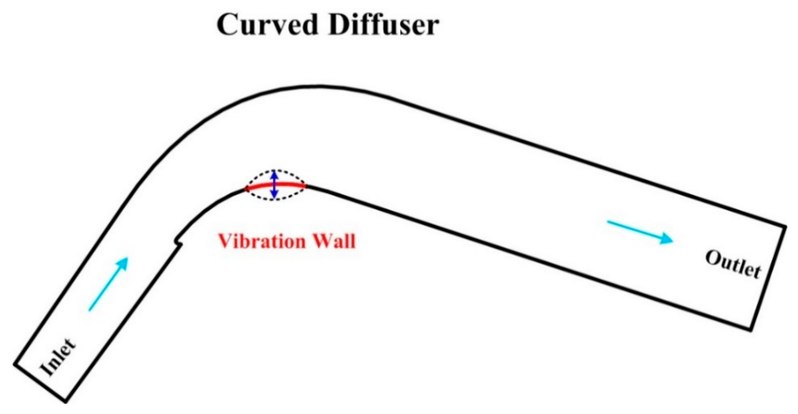
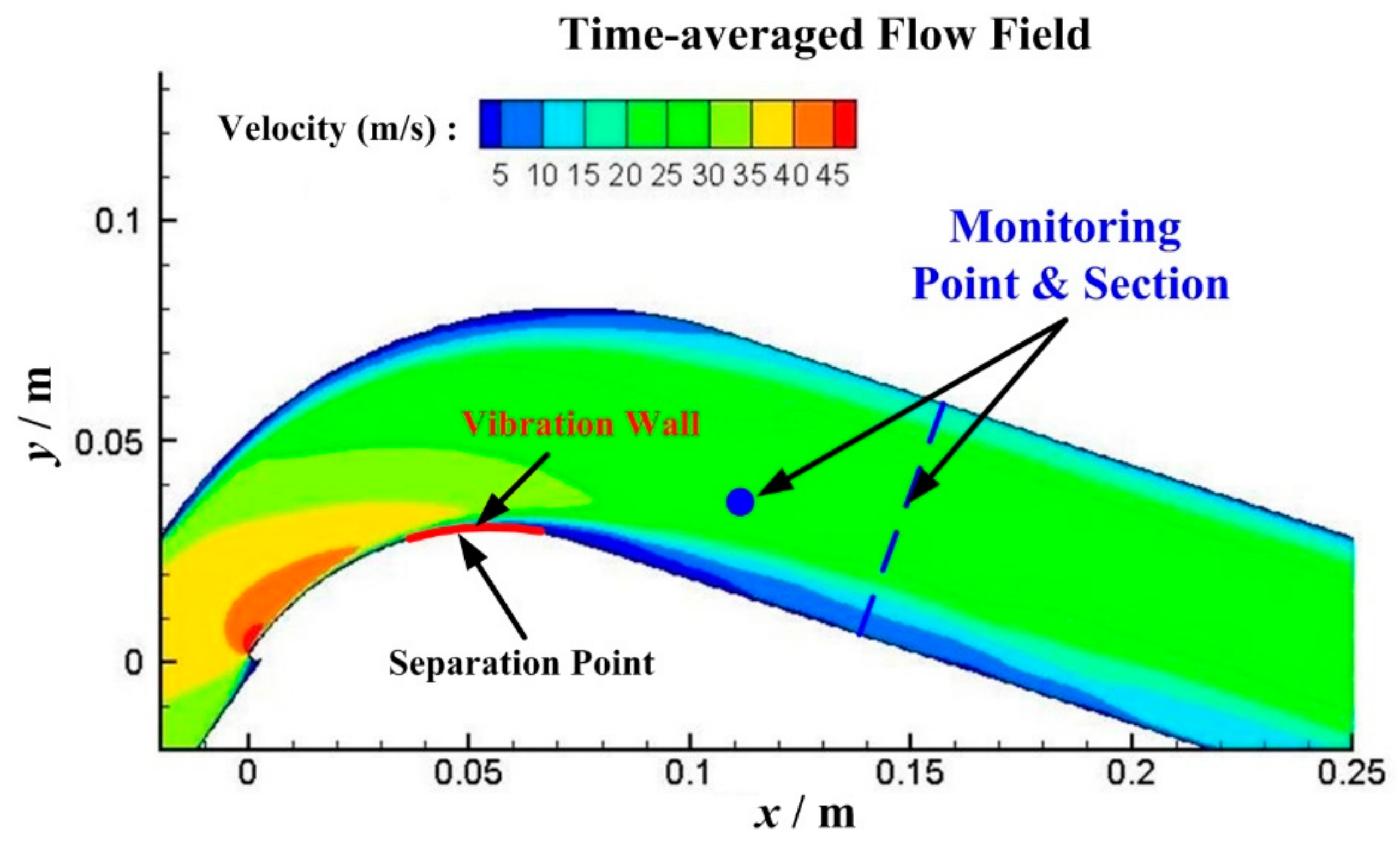
3. CFD Method of Flow Separation Control by a Vibration Wall in a Curved Diffuser

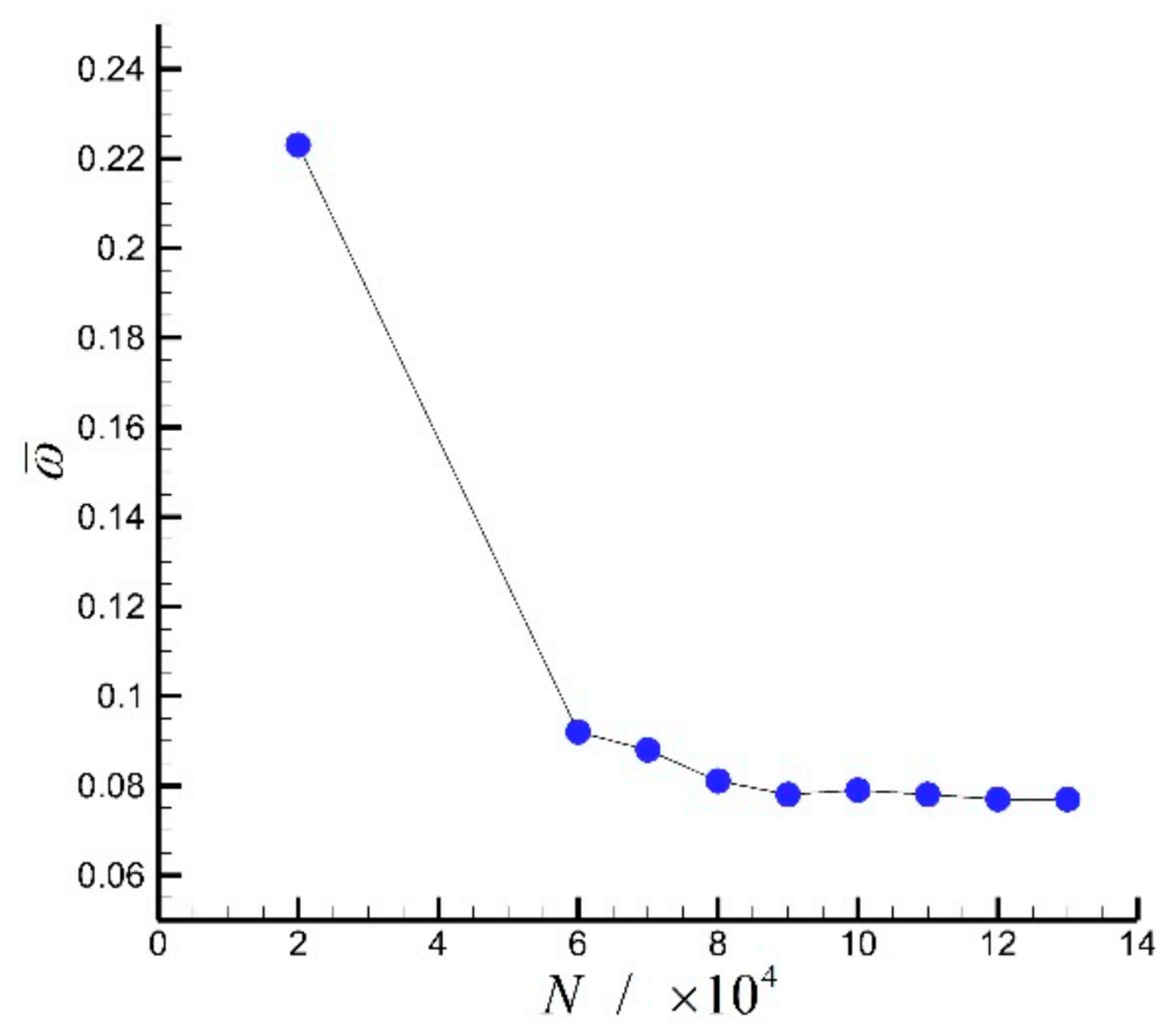
3.1. Introduction of the Numerical Method

Vibration wall control is used for a curved diffuser (as shown in Figure 4) with typical flow separation in this paper. The diffuser includes an inlet, a curved part and an outlet. The inlet width, outlet width and chord length of the curved part are 34.3 mm, 55 mm and 80 mm, respectively. Large eddy simulation (LES) with Smagorinsky–Lilly sub-grid model is chosen by us for the numerical simulation. The inlet Mach number, determined by the inlet total pressure and exit static pressure, is set as 0.1 in all cases, to avoid potential compressible effect which functions when the Mach number exceeds 0.3. Dual-time stepping is used to solve the unsteady process and the physical time step is set as 10⁻⁵ s. After the grid-independent study [18] (as shown in Figure 5), the grid number used is about 8 × 10⁴ considering of both computational accuracy and economy. More details of the numerical method and some of the numerical results can be found in Ref. [19].

The vibration wall is realized in the simulation by the dynamic mesh technique with a spring-based smoothing model. The function of the vibration wall is described as a stationary wave realized by a user defined function (UDF), shown as:

$$y(x,t)=y_0(x)+A_e\sin (2\mathsf{\pi }{f}_{e}t)\sin (\mathsf{\pi }\frac{x-x_0}{L}) x_0<x<x_0+L$$

(24)

where $y_0(x)$ is used to describe the lower surface of the diffuser geometry and $x_0$ is the starting position of the vibration wall; while $A_e$, $f_e$ and $L$ are the amplitude, frequency and length of the vibration wall. $A_e$ and $f_e$ are adjustable because excitation frequency and intensity have shown great impact on control performance in previous works of unsteady flow control by others, while other parameters are fixed ($L=30 \mathrm{mm}$) in this study.

3.2. Nondimensional Parameters of the Vibration Wall

Before exploring the characteristics of flow control by a vibration wall, we firstly define some nondimensional parameters for describing the vibration wall control. The nondimensional vibration frequency is defined as:

$$F^{+}=f_e/f_0$$

(25)

where $f_e$ is the vibration frequency and $f_0$ is the dominant vortex frequency in the uncontrolled flow field. $f_0$ is 360 Hz in this case via fast Fourier transform (FFT) analysis.

Another parameter to describe the vibration wall is the nondimensional vibration amplitude, which is defined as:

$$A^{+}=A_e/L_0$$

(26)

where $A_e$ is the vibration amplitude and $L_0$ is the estimated vortex radius (about 0.01 m in this case) in the uncontrolled flow field.

3.3. Evaluation Indexes

To evaluate the control performance, we define a nondimensional index called the relative saving of the total pressure loss. The total pressure loss coefficient $\omega$ is widely used and defined as:

$$\omega =\frac{P_1^{*}-P_2^{*}}{0.5\rho V_1^2}$$

(27)

where $P_1^{*}$ is the inlet total pressure, $P_{{}_2}^{*}$ is the outlet total pressure, $\rho$ is the density, and $V_1$ is the inlet velocity. Then, the relative saving of the total pressure loss $\tilde{\omega }$ is defined as:

$$\tilde{\omega }=\frac{{\omega }_{\mathrm{n}}-{\omega }_{\mathrm{c}}}{{\omega }_{\mathrm{n}}}$$

(28)

where ${\omega }_{\mathrm{n}}$ and ${\omega }_{\mathrm{c}}$ are the total pressure loss coefficients of the curved diffuser with no control and with vibration wall control, respectively. This index reflects the control performance in terms of mechanical energy saving.

Moreover, degree of order is of importance in nonlinear dynamics and effective external excitation seems to have the ability to change the degree of order of a flow field [20]. A classic index to evaluate the degree of order is the maximal Lyapunov exponent. In a discrete or continuous dynamic system, two phase points will diverge or converge in the iterative or evolutionary process, and Lyapunov exponent is an indicator to quantitatively describe this process. There are n Lyapunov exponents in a n-dimensional dynamic system. When one positive Lyapunov exponent exists, the system tends to be chaotic, while when all of the Lyapunov exponents are negative, the system tends to be orderly. So, the maximal Lyapunov exponent is an effective index to evaluate the degree of order of a dynamic system. The $i$th Lyapunov exponent ${\lambda }_i$ is defined as:

$${\lambda }_i=\underset{t\to \infty }{\lim }\underset{\epsilon (0)\to 0}{\lim }\frac{1}{t}\ln \left|\frac{{\epsilon }_i(t)}{\epsilon (0)}\right|$$

(29)

where $\epsilon (0)$ is the radius of an n-dimensional infinitesimal sphere, which evolves into an n-dimensional ellipsoid over time, of which ${\epsilon }_i(t)$ is the $i$th dimension semimajor axis [21]. When ${\lambda }_i$ is sorted by value (from largest to smallest), ${\lambda }_1$ is the largest and referred as the maximal Lyapunov exponent. The maximal Lyapunov exponent is calculated based on the time series of monitoring points from the simulation. To be exact, the C-C algorithm and Wolf method are used for the reconstruction of the phase space and then the calculation of ${\lambda }_1$ (See Ref. [21] for more details).

4. Comparison of Model-Based and CFD Results

4.1. Vibration Frequency Analysis

As shown in Figure 6, when the vibration wall is off, a time-averaged flow separation zone occurs on the suction side of the curved diffuser. The vibration wall is designed near the separation point, because the separation vortex is easier to change at its growing stage. Then, we study the effect of vibration frequency on the control performance. In the CFD simulation, the nondimensional vibration amplitude $A^{+}$ maintains 0.1 and the nondimensional vibration frequency $F^{+}$ (defined in Equation (25)) is variable. Meanwhile, in the model, the external excitation intensity $A_e$ maintains 0.05 and the nondimensional excitation frequency ${\omega }_e{}^{+}$ is variable and defined as:

$${\omega }_e{}^{+}={\omega }_e/{\omega }_0$$

(30)

The control performance of the vibration wall under different nondimensional excitation frequencies is shown in Figure 7, containing both the CFD and model results. It is obvious that when the nondimensional excitation or vibration frequency is around 1, the control performance reaches its maximum (the relative saving of the total pressure loss is about 18%). This frequency-dependent phenomenon is also reported in other’s works [2]. To be explicit, in the CFD results, high relative saving of the total pressure loss means much of the energy loss due to flow separation is restored by the vibration wall, while in the model-based results, high entrainment degree means much momentum from the mainstream is transferred to the separation zone due to external excitation. It should be noted that the natural frequency of separation vortex is the most unstable frequency of the flow field. So, the control performance optimization when the vibration wall frequency equals the dominant frequency of separation vortex ($F^{+}=1$) must be related to flow instability. Combining the CFD and model results, we can infer that the separation vortex is promoted and serves as a medium for momentum transfer when the vibration wall frequency is tuned.

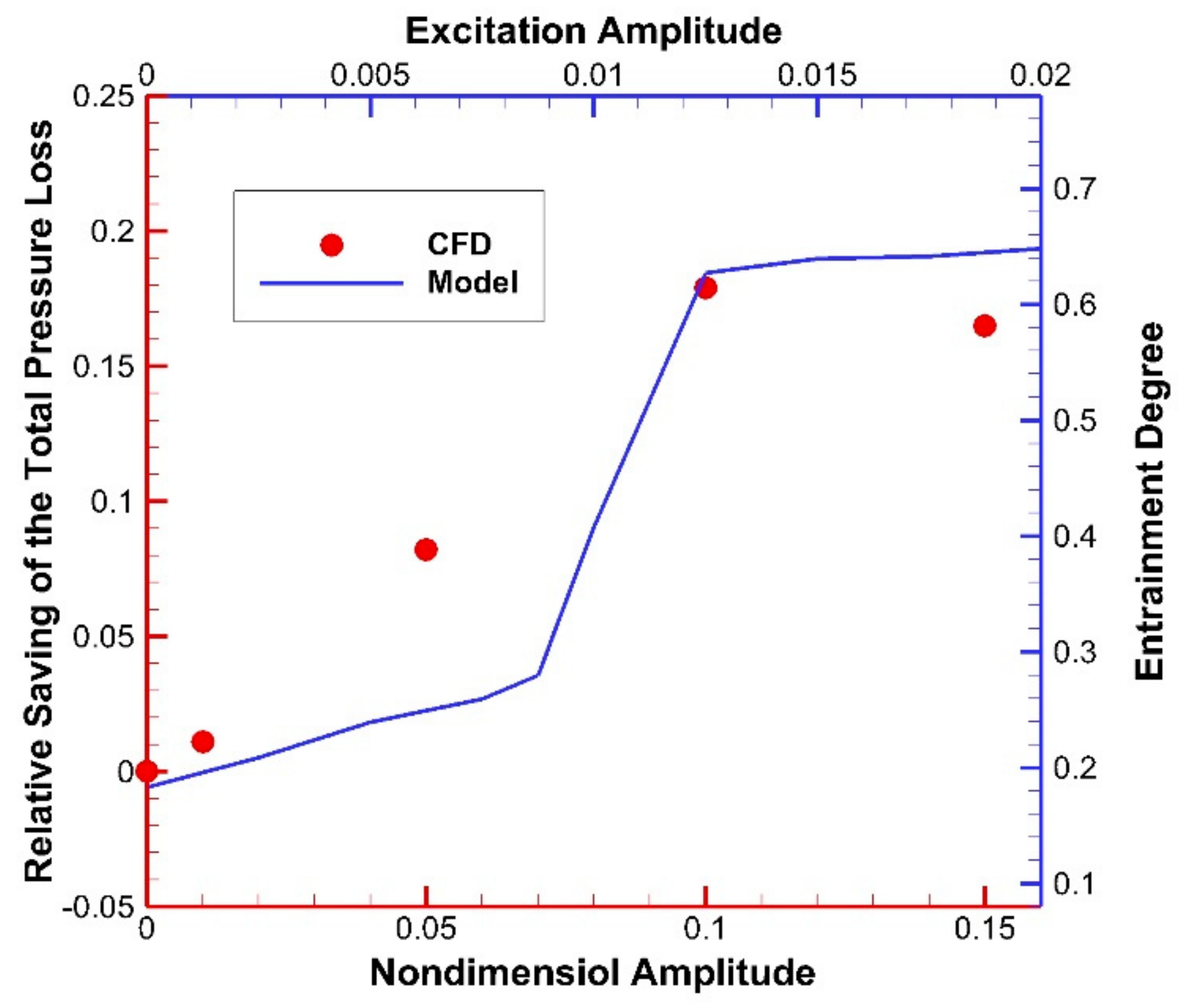
4.2. Vibration Amplitude Analysis

In this section, we study the effect of the vibration amplitude on the control performance. Figure 8 shows both the CFD and Model results by changing the nondimensional vibration amplitude $A^{+}$ and the external excitation intensity $A_e$ ($F^{+}$ and ${\omega }_e{}^{+}$ maintain 1). As illustrated in Figure 8, the CFD results show that as the nondimensional vibration amplitude increases, the relative saving of the total pressure firstly increases and then decreases, implying an optimal nondimensional amplitude about 0.1. Meanwhile, in the model-based results, as the excitation amplitude increases, the entrainment degree also increases firstly but then does not change a lot when $A_e>0.0125$. So, according to the model, the momentum transferred by the separation vortex increases with the vibration amplitude firstly, but it is restricted then. As the model indicates, when the vibration amplitude exceeds a threshold, no more momentum will be transferred through the unsteady separation vortex. However, as the CFD results show, an excessive vibration amplitude will result in more energy losses, which may be caused by unnecessary y-direction disturbance on the mainstream.

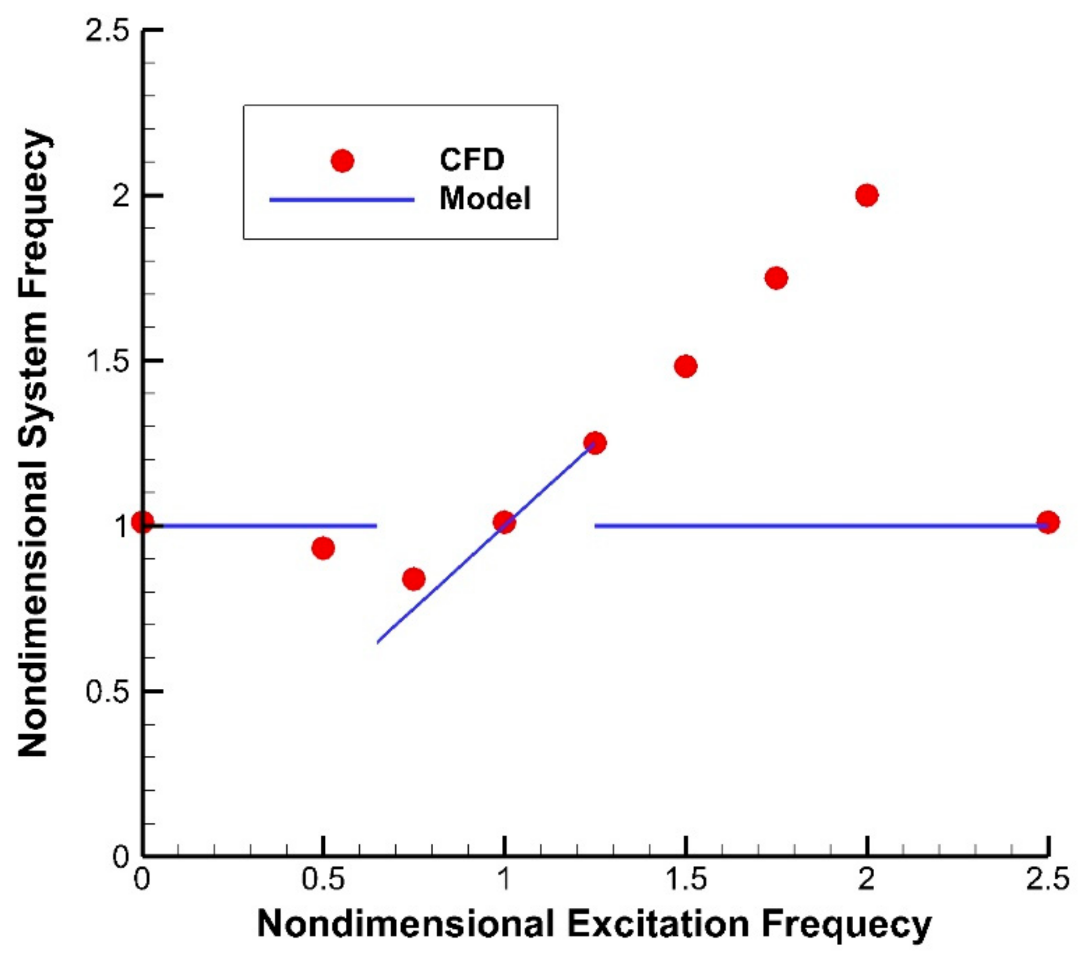
4.3. Lock-In Analysis

One reason that external excitation such as that from a vibration wall functions is that it can lock in the fluid system. This means the forced external periodic excitation can interact with the intrinsic self-excited motion under certain conditions. Figure 9 shows the relationship between the dominant system frequency and the nondimensional excitation frequency. For the CFD results, the dominant system frequency is obtained by FFT of the static pressure at the monitoring point (as shown in Figure 6) and the nondimensional external excitation is $F^{+}$. Moreover, for the model results, the dominant system frequency is obtained by FFT of the dynamic system, and the nondimensional external excitation is ${\omega }_e{}^{+}$. As shown in Figure 9, we can clearly see a frequency lock region. And this region is approximately $0.65<{\omega }_e<1.25$ in the model-based results, while approximately $0.75<F^{+}<2$ in the CFD results. So, the lock-in region in the CFD results is wider than the model predicts when on the right side of $F^{+}=1$. According to the vibration frequency analysis, the control performance optimizes when $F^{+}=1$. Thus, we think lock-in may be a precondition for effective vibration wall flow control.

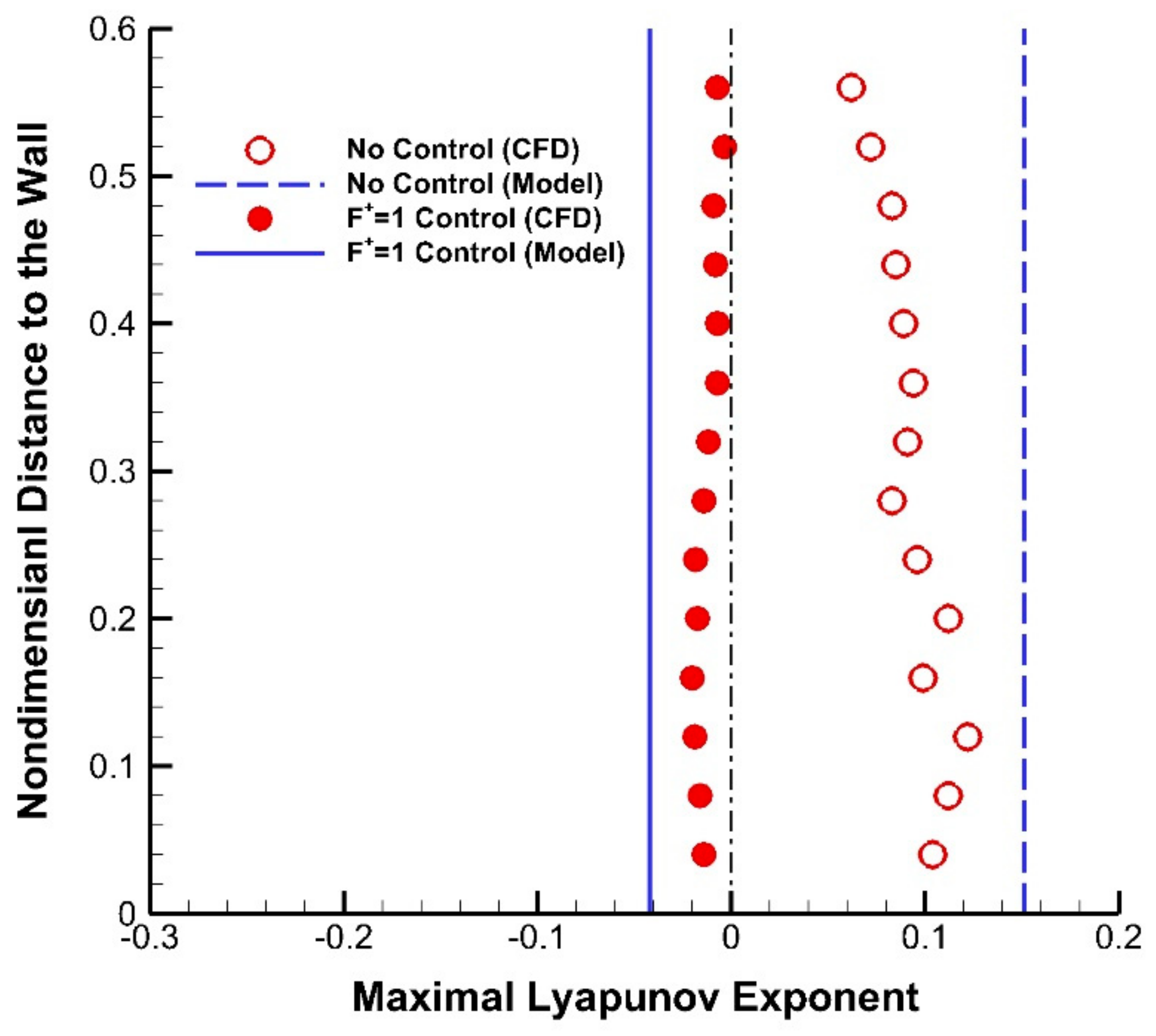
4.4. Degree of Order Analysis

In order to evaluate the degree of order of the flow field, the maximal Lyapunov exponents obtained by time series analysis of the pressure on the monitoring section of the curved diffuser without control and with $F^{+}=1$ control (as shown in Figure 6) are illustrated in Figure 10. Also, the maximal Lyapunov exponents calculated by the model are added to Figure 10 for comparison. So, the CFD results generally agree with the model-based predictions, that the maximal Lyapunov exponents of the uncontrolled flow field are positive (indicating chaotic), while the maximal Lyapunov exponents of the flow field under effective control are negative (indicating ordered). Thus, the results show that vibration wall with proper parameters can make the flow field evolve from a chaotic one to a more orderly one. This can also be seen from the instantaneous flow fields in Figure 11, as the uncontrolled flow field contains more disordered small-scale vortices, while the flow field with effective vibration wall control is only dominated by ordered large-scale vortices.

5. Discussion

In this paper, a nonlinear simplified model was established based on the 2D incompressible N-S equation, Oseen vortex model, and K-H instability. The behaviors of the model agree with what we found in vibration wall flow control. Thus, cued by both the model and the CFD results, the mechanism of vibration wall flow control can be discussed here.

In the degree of order analysis, according to both the model and CFD results, it implies that a vibration wall with tuned parameters is able to change the flow field from a disordered one into an ordered one. Moreover, from the vibration frequency analysis, we know tuned parameters of a vibration wall can also maximized momentum transfer. So, we think the mechanism of vibration wall flow control is that it helps to reduce time-averaged flow separation via momentum transfer, and it also helps unsteady separated vortices to travel more efficiently (in a more orderly way). In short, vibration wall control with fine parameters can maximize momentum transfer and make the flow field in a less chaotic and low-loss state.

Another issue regarding vibration wall control concerns how to realize tuned parameters. According to the lock-in analysis, it seems that the lock-in may be a precondition for effective vibration wall flow control. In another word, the periodic excitation a vibration wall produces must dominate in an unsteady separated flow field before it functions. And this is also proven by the vibration amplitude analysis that the intensity of vibration must be strong enough to result in effective flow control. Also, in the vibration frequency analysis, it is found that the optimum vibration frequency is around the frequency of separated vortices. This implies the economic way (the energy cost grows larger with the increase of vibration amplitude) to actuate the vibration wall must utilize flow instability, because the dominant separated vortices themselves are stimulated by the most unstable mode in the flow stability theory.

According to this discussion, the simplified model helps us understand the behaviors of vibration wall flow control, and guide the design and application of it. Although the model cannot describe the behaviors of vibration wall flow control very accurately for now, we hope to develop this model in the future and improve its accuracy. When this model is mature enough, it will support the construction of a rapid design platform for preliminarily designing vibration walls in flow control and save plenty of time of parameter optimization through simulations or experiments.

6. Conclusions

The effect of vital control parameters for vibration wall in a curved diffuser is studied by numerical simulation (CFD) and analyzed based on a nonlinear simplified model. The outcomes of the model agree with the CFD results qualitatively, helping us to understand the phenomena and mechanisms in vibration wall control. The main conclusions are as follows:

1. In order to explain the phenomena and mechanisms in vibration wall control, a simplified nonlinear model is established based on the 2D incompressible N-S equation, Oseen vortex model and K-H instability. The complete form of the model is shown as: $\left\{\begin{array}{l}\frac{d^{2}y}{d{t}^2}=-ay-c{y}^3-e\frac{dy}{dt}+f\\ \frac{d^{2}f}{d{t}^2}=-{\omega }_0^{2}f+2(\sigma -4l{f}^2)\frac{df}{dt}+A_e\sin ({\omega }_{e}t)\end{array}\right.$. In this model, the frequency and amplitude of the vibration wall are modeled as ${\omega }_e$ and $A_e$, respectively. Then, the control performance is evaluated by entrainment degree $\sigma$.

2. Both the CFD and model-based analysis shows that when the vibration frequency is around the system frequency, the control performance optimizes, and the vibration frequency tends to lock-in the system frequency. This infers that the lock-in may be a precondition for effective vibration wall flow control and effective vibration frequency will use the separation vortex as a medium to strengthen the momentum transfer from the mainstream to the separation zone.

3. Both the CFD and model-based analyses indicate an optimum vibration amplitude. As the excitation amplitude increases, the momentum transfer from the mainstream to the separation zone will also increases and results in better control performance. But momentum transfer through the separation vortex has its limitation. An excessive vibration amplitude will bring more energy losses and relatively poor control performance.

4. By analyzing the maximal Lyapunov exponents, both the CFD and model-based analyses imply that the vibration wall with tuned parameters is able to change the flow field from a disordered one into an ordered one. Combining this with maximized momentum transfer, effective vibration wall control will support the flow field in a less chaotic and low-loss state.

References

1. Telionis, D.P. Review—Unsteady boundary layers, separated and attached. J. Fluids Eng. 1979, 101, 29–43. [Google Scholar] [CrossRef]
2. Greenblatt, D.; Wygnanski, I.J. The control of flow separation by periodic excitation. Prog. Aerosp. Sci. 2000, 36, 487–545. [Google Scholar] [CrossRef]
3. Nishioka, M.; Asai, M.; Yoshida, S. Control of Flow Separaion by Acoustic Excitation. AIAA J. 1987, 28, 1909–1915. [Google Scholar] [CrossRef]
4. Glezer, A.; Amitay, M. Synthetic jets. Annu. Rev. Fluid Mech. 2002, 34, 503–529. [Google Scholar] [CrossRef]
5. Wang, Y.; Zhou, P.; Yang, J. Parameters effect of pulsed-blowing over control surface. Aerosp. Sci. Technol. 2016, 58, 103–115. [Google Scholar] [CrossRef]
6. Ebrahimi, A.; Hajipour, M. Flow separation control over an airfoil using dual excitation of DBD plasma actuators. Aerosp. Sci. Technol. 2018, 79, 658–668. [Google Scholar] [CrossRef]
7. Wu, X.H.; Wu, J.Z.; Wu, J.M. Streaming effect of wall oscillation to boundary layer separation. In Proceedings of the 29th Aerospace Sciences Meeting, Reno, NV, USA, 7–10 January 1991. [Google Scholar]
8. Sinha, S.; Hyvärinen, J. Flexible-Wall Turbulence Control for Drag Reduction Streamlined and Bluff Bodies. In Proceedings of the 4th Flow Control Conference, Seattle, WA, USA, 23–26 June 2008. [Google Scholar]
9. Yang, R.; Zhong, D.; Ge, N. Numerical investigation on flow control effects of dynamic hump for turbine cascade at different Reynolds number and hump oscillating frequency. Aerosp. Sci. Technol. 2019, 92, 280–288. [Google Scholar] [CrossRef]
10. Kang, W.; Xu, M.; Yao, W.; Zhang, J. Lock-in mechanism of flow over a low-Reynolds-number airfoil with morphing surface. Aerosp. Sci. Technol. 2020, 97, 105647. [Google Scholar] [CrossRef]
11. Zheng, X.Q.; Zhou, X.B.; Zhou, S. Investigation on a type of flow control to weaken unsteady separated flows by unsteady excitation in axial flow compressors. J. Turbomach. 2005, 127, 489–496. [Google Scholar] [CrossRef]
12. Collis, S.S.; Joslin, R.D.; Seifert, A.; Theofilis, V. Issues in active flow control: Theory, control, simulation, and experiment. Prog. Aerosp. Sci. 2004, 40, 237–289. [Google Scholar] [CrossRef]
13. Orszag, S.A. Accurate solution of the Orr-Sommerfeld stability equation. J. Fluid Mech. 1971, 50, 689–703. [Google Scholar] [CrossRef] [Green Version]
14. Drazin, P.G.; Reid, W.H. Hydrodynamic Stability, 2nd ed.; Cambridge University Press: Cambridge, UK, 2004. [Google Scholar]
15. Batcheler, G.K. An Introduction to Fluid Dynamics; Cambridge University Press: Cambridge, UK, 1967. [Google Scholar]
16. Kovacic, I.; Brennan, M.J. The Duffing Equation: Nonlinear Oscillators and Their Behavior; John Wiley & Sons: Hoboken, NJ, USA, 2011. [Google Scholar]
17. Stuart, J.T. On the non-linear mechanics of hydrodynamic stability. J. Fluid Mech. 1958, 4, 1–21. [Google Scholar] [CrossRef]
18. Lu, W.; Huang, G.; Wang, J.; Yang, Y. Flow Separation Control in a Curved Diffuser with Rigid Traveling Wave Wall and Its Mechanism. Energies 2019, 12, 192. [Google Scholar] [CrossRef] [Green Version]
19. Wang, J.C.; Fu, X.; Huang, G.P.; Hong, S.L.; Zou, Y.C. Application of the Proper Orthogonal Decomposition Method in Analyzing Active Separation Control with Periodic Vibration Wall. Int. J. Turbo Jet Engines 2019, 36, 175–184. [Google Scholar] [CrossRef]
20. Lu, W.; Huang, G.; Zhu, J.; Fu, X.; Wang, J. A nonlinear dynamic model for unsteady separated flow control and its mechanism analysis. J. Fluid Mech. 2017, 826, 942–974. [Google Scholar]
21. Wolf, A.; Swift, J.B.; Swinney, H.L.; Vastano, J.A. Determining lyapunov exponents from a time series. Phys. D Nonlinear Phenom. 1985, 16, 285–317. [Google Scholar] [CrossRef] [Green Version]
Figure 1. A vortex row with a pair of symmetric small-scale vortices.
Energies 14 01781 g001
Figure 2. Diagram for modeling the dissipation term inside a small-scale vortex.
Energies 14 01781 g002
Figure 3. Evolutionary process from a vortex sheet to a concentrated vortex row due to K-H Instability.
Energies 14 01781 g003
Figure 4. Curved Diffuser and the vibration wall.
Energies 14 01781 g004
Figure 5. Grid-independent study (loss coefficient vs. grid number) [18].
Energies 14 01781 g005
Figure 6. Time-averaged flow field of the curved diffuser when the vibration wall is off.
Energies 14 01781 g006
Figure 7. Control performance of the vibration wall vs. nondimensional excitation frequency (CFD [19] and Model results).
Energies 14 01781 g007
Figure 8. Control performance of the vibration wall vs. excitation amplitude (CFD [19] and Model results).
Energies 14 01781 g008
Figure 9. Nondimensional system frequency vs. Nondimensional excitation frequency (CFD and Model results).
Energies 14 01781 g009
Figure 10. Maximal Lyapunov exponents without control and with F + = 1 control (CFD [19] and Model results).
Energies 14 01781 g010
Figure 11. Instantaneous vorticity contour of the flow fields in the curved diffuser: (a) no control; (b) with F + = 1 control.
Energies 14 01781 g011