Abstract
The integration and control of energy systems for power generation consists of multiple heterogeneous subsystems, such as chemical, electrochemical, and thermal, and contains challenges that arise from the multi-way interactions due to complex dynamic responses among the involved subsystems. The main motivation of this work is to design the control system for an autonomous automated and sustainable system that meets a certain power demand profile. A systematic methodology for the integration and control of a hybrid system that converts liquefied petroleum gas (LPG) to hydrogen, which is subsequently used to generate electrical power in a high-temperature fuel cell that charges a Li-Ion battery unit, is presented. An advanced nonlinear model predictive control (NMPC) framework is implemented to achieve this goal. The operational objective is the satisfaction of power demand while maintaining operation within a safe region and ensuring thermal and chemical balance. The proposed NMPC framework based on experimentally validated models is evaluated through simulation for realistic operation scenarios that involve static and dynamic variations of the power load.
1. Introduction
Carbon dioxide (CO2) emission reduction is a major goal on a global scale. Autonomous mobile power generation systems mainly rely on diesel generators that are both polluting and fossil fuel dependent [1]. On the other hand, power generation via hydrogen from renewable sources is a competitive alternative. Fuel cells are electrochemical devices that convert the chemical energy of a fuel directly into electricity and their technological nature has reached a level that makes them suitable for widespread industrial use. Their connectivity with renewable energy sources and energy carriers, such as hydrogen, renders them as the energy conversion devices of the future that can contribute to the sustainable development of the energy and transport sectors, especially for autonomous and mobile applications. Common examples of such applications are autonomous portable charging stations (for electric scooters, bikes, or electric boats and forklifts, etc.), and off-grid power generation small scale systems (campers and applications that could replace traditional diesel generators, such as food carts). Moreover, applications that require low-noise portable power generation find a very fitting solution in these systems. Autonomous power systems involve the integration of hydrogen production from an easy to store and transport source with a fuel cell (FC) for electricity power generation. A thermal balance between the chemical conversion to H2 and the fuel cell is important for efficient operation. High-temperature proton exchange membrane fuel cells (HT-PEMFC) that use phosphoric acid doped polybenzimidazole (PBI) membranes can operate at temperatures up to 200 °C [2]. The benefits of operation at these elevated temperatures are mainly the tolerance to carbon monoxide (CO) concentrations in the hydrogen feed stream, commonly present when operating with reformate streams that can be increased by many orders of magnitude compared to that of a low-temperature proton exchange membrane fuel cell (LT-PEMFC). Furthermore, water management is better handled, since the water is in a vapor state and since PBI membranes are conductive at very low relative humidity, no moisture control is needed. Moreover, the high working temperature eliminates the possibility of water condensation in pores or channels of the fuel cell. Due to the higher temperature difference compared to the surroundings, thermal management can be satisfactorily performed by a smaller cooling system [3].
Several research studies have been carried out regarding the development of fuel cell-based hybrid power systems that utilize reformed hydrogen. Such power systems are designated to work as charging stations, auxiliary power units (APU), or uninterruptible power supply units (UPS). In general, integrated fuel cell systems exhibit slow dynamics related to the feed stock reform to hydrogen, and fast dynamics associated with the fuel cell and battery. Uncertainties associated with catalyst deactivation and membrane malfunction commonly affect system performance.
Most of the recent research efforts regarding model-based predictive control have been focused on systems whose main power generating unit is a LT-PEMFC. Within this scope, a nonlinear dynamic model and a model predictive control (MPC) framework for an LT-PEMFC is presented in [4]. A linearized model is used in MPC in order to track the desired output fuel cell voltage trajectory. To improve the efficiency and durability of LT-PEMFC based power systems simultaneously, an nonlinear model predictive control (NMPC) strategy is proposed [5] in order to deliver the specified load, while ensuring maximum efficiency and avoiding local starvation and inappropriate water accumulation in the compartments. This strategy showed improved results in comparison with a fixed stoichiometry control strategy for the fuel cell. An NMPC strategy that ensures maximum efficiency of an LT-PEMFC power system by maximizing the electrochemically active surface area is proposed in [6]. To guarantee lifetime enhancement of the LT-PEMFC, the designed controller imposes operational constraints to avoid hydrogen and oxygen starvation at the anode and cathode compartments, respectively. The research team in [7] addresses the real-time application of NMPC for the efficiency improvement of an LT-PEMFC power system. They consider the fuel cell stack current, the anode hydrogen flow, and the cathode oxygen flow as decision variables for their controller. The control of the exhaust gas of an LT-PEMFC with NMPC is presented in [8]. The goal was to achieve the production of dehumidified and oxygen-depleted air in the exhaust so that the system can serve as an APU for the electrical power supply on an aircraft. Another study [9] involved the design of a multi-input-multi-output nonlinear state feedback controller in order to maintain adequate hydrogen supply and suitable anode hydrogen concentration under variable load demands. The design of an NMPC controller for an LT-PEMFC power system that also utilizes a small lithium-ion battery as a buffer power supply was presented in [10]. The proposed power management strategy managed the power demand for the fuel cell and the battery to improve the response to dynamic load changes and ensure the safe operation of the battery.
A limited number of control strategies have been proposed in the literature that deal with hybrid HT-PEMFC or LT-PEMFC systems that utilize hydrogen production via reforming. The research team in [11] developed energy management strategies for a combined heat and power plant using HT-PEMFCs and methane reforming. Three different strategies were proposed and implemented. Fuel supply variations alone were considered in the first strategy, fuel cell current density variations in the second, and both fuel supply and current density variations in the third strategy. They resulted in a power generation map showing the trade-off between thermal and electrical power generation, while operating at different load levels. The same research group [12] employed a multi-objective optimization using a genetic algorithm in order to optimize the design and operating variables of an HT-PEMFC. They considered the net electrical efficiency and capital cost as optimization objectives and selected the current density, steam to carbon ratio, burner outlet temperature, and the auxiliary to process fuel ratio as design parameters. In an extension of this work [13], a multi-objective optimization approach was employed to determine the optimal operating parameters for a range of 15,000 h of operation of an HT-PEMFC-based combined heat and power plant. Two different objective functions were utilized, one accounting for the net electrical efficiency and thermal generation and the other for the net electrical efficiency and electrical power generation. The results demonstrated a superior performance compared to previous works. In a similar study [14], the net electrical and thermal efficiencies were considered as objectives to provide multiple optimal operating conditions at various electrical and thermal generation levels using models developed in [15]. Finally, there have been studies dealing with the mathematical description and control analysis of a methanol autothermal reformer/LT-PEMFC autonomous system [16,17]. Analytical models of the components have been developed and used in the formulation of alternative flowsheets in order to evaluate their response to multiple simultaneous disturbances. Dynamic models for a similar autonomous power system that consists of a liquefied petroleum gas (LPG) steam reformer, an HT-PEMFC, and a Li-ion accumulator have been proposed.
In general, integrated HT-PEMFC with hydrogen production via reforming is a complex system with various and complex phenomena evolving during operation, which poses challenging control issues. Characteristics such as the large range of dynamic responses among the various multi-way subsystem interactions and potentially conflicting operating objectives, are to be confronted through the development of an advanced control framework. The incentive for efficient control of an integrated hydrogen production fuel cell system is the improvement of its overall performance, the increase in durability for process equipment, and safety for use in stationary and mobile applications. Additionally, it is important to ensure safe and economical operation by avoiding oxidant starvation, while minimizing hydrogen consumption. Such control issues cannot be addressed by conventional single-loop control structures, and therefore, advanced control techniques, such as NMPC can achieve the optimal satisfaction of multiple objectives. NMPC possesses the ability to handle state and input constraints, nonlinearities, the process dynamic behavior explicitly, and to balance the thermal and material resources in the entire system in a holistic way.
Most of the research studies implement or propose control strategies for hybrid systems that are based on LT-PEMFC and rely on single feedback loops that do not take into account the system interactions efficiently. In addition, the current work considers systems that combine fuel reforming and fuel cell systems in an integrated way. A model-based predictive control framework is, therefore, necessary to handle multiple time scales in system response and strong interactions that may be built among the associated subsystems. To this end, a nonlinear semi-empirical model that takes into consideration the operating constraints imposed by each subsystem is employed for the fuel cell and is experimentally validated on an existing unit operating in the Chemical Process Engineering and Energy Resources Institute (CPERI) at the Centre for Research and Technology Hellas (CERTH). An efficient control struct is determined along with a reasonable optimization framework that reflects on the system objectives.
The paper is organized as follows: Section 2 provides a detailed description of the flow diagram of the plant setup and Section 3 presents the mathematical models for each subsystem and their validation. Section 4 outlines the NMPC control framework along with the optimization methodology. Finally, Section 5 discusses the simulation results of the proposed NMPC framework and the achieved performance of the system.
2. System Description and Mathematical Modeling
This section presents an overview of the integrated unit under consideration. Figure 1 depicts a basic flow diagram of the hybrid system and its subsystems which are the LPG reformer, the HT-PEMFC, the Li-ion battery stack, and the load. The actual unit that operates in CPERI/CERTH is illustrated in Figure 2 alongside the supervisory control and data acquisition (SCADA) system that is installed for the operation needs.
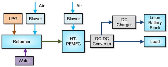
Figure 1.
Topology and main components of the hybrid system [18]. DC: direct current; DC-DC: direct current to direct current.
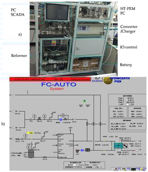
Figure 2.
Pictures showing the integrated system and its human machine interface: (a) test unit; (b) supervisory control and data acquisition system (SCADA).
The load requirements are mainly covered by the battery, which is charged by the HT-PEMFC integrated with the LPG reformer. However, the HT-PEMFC can directly provide the necessary power if the battery charge level is low. The necessary hydrogen for the fuel cell is produced by the fuel reformer but can alternatively originate from pressurized hydrogen tanks. For the scope of this study, the hydrogen is considered to originate only from the reformer. Specifications for the system components are depicted in Table 1.

Table 1.
System specifications.
Figure 3 shows a detailed overview of the subsystems of the LPG reformer and its connection to the HT-PEMFC. The main flow streams are represented by different lines in the diagram which are: single dot-dash for the flow of H2 or hydrogen-rich gas, double dot-dash for the flow of LPG, grey for the flow of water (liquid, steam, or both), and black for air or flue gas.
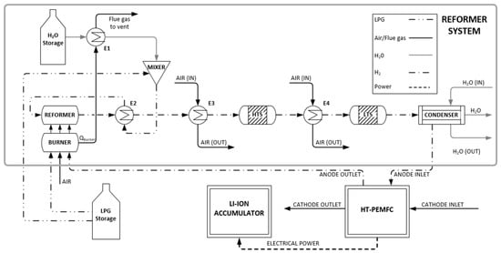
Figure 3.
Flow diagram of the integrated power generation system.
Initially, the LPG stream from the storage tank is split into two streams, one feeding the burner with the necessary fuel and one going to the reformer to be processed. The first stream enters the burner alongside air and the remaining hydrogen from the anode outlet. This mixture combusts to provide the heat required to start the endothermic reactions in the reformer. The flue gas leaves the combustion chamber at high temperatures and provides the thermal energy which is utilized in the superheater to separate superheated steam for the reforming reactions. The steam stream is then mixed with the LPG stream from the tank. This mixture is heated by a heat exchanger that utilizes the high temperature of the reformer outlet stream. After the reforming reactor, the resulting product is a hydrogen-rich reformate gas that also includes CO, CO2 and a fraction of the feed that did not react. Although the HT-PEMFC has a high CO tolerance, the CO concentration as the gas leaves the reformer is still too high to be fed directly to the fuel cell. As a result, the reformer outlet stream is introduced to the water–gas shift reactors to reduce the CO concentration at the desired level, through its conversion to H2. The temperature of the stream entering the first high-temperature shift (HTS) reactor is brought down primarily by the feed-effluent heat exchanger E2 and then by the air-cooled E3. The HTS downstream heat exchanger E4 regulates the temperature of the feed stream to the low-temperature shift (LTS) reactor which further reduces the CO concentration to an acceptable level. Prior to the fuel cell’s anode inlet, there is a water management system that reduces the water content in the reformate gas. The condenser uses water to cool down the gas stream and remove water from it. The hydrogen-rich reformate gas enters the anode inlet at the desired temperature and CO concentration. The hydrogen stream enters the cathode where it releases its electrons for the generation of electric power. Hydrogen ions are transferred through the proton-exchange membrane and they react with oxygen in the anode to produce H2O. A DC-DC converter regulates the voltage of the electric current of the fuel cell. The Li-ion battery and the load are connected to the DC bus.
2.1. Model for the LPG Reformer
In the present study, to provide the required hydrogen for the electrochemical reaction in the fuel cell, a heat integrated wall reactor LPG reformer was incorporated. The characteristics and dynamics of the above reformer originate from operational data of an experimental unit at CPERI/CERTH that result from conducted experiments. The proposed model aims to simulate the response of the reformer to a change in the hydrogen demand. The reformer’s equation is approximated by a fourth-order linear system as below:
where is the system’s output variable that represents the reformer output flow of hydrogen entering the anode channel of the fuel cell, is the system’s command variable and represents the demanded flow of hydrogen in the fuel cell, is the gain and are parameters in the differential equation of the reformer. Figure 4 illustrates the experimental output response of the reformer system to a step change from 0 to 1 l/min in comparison with the hydrogen flow calculated by the reformer’s equation.
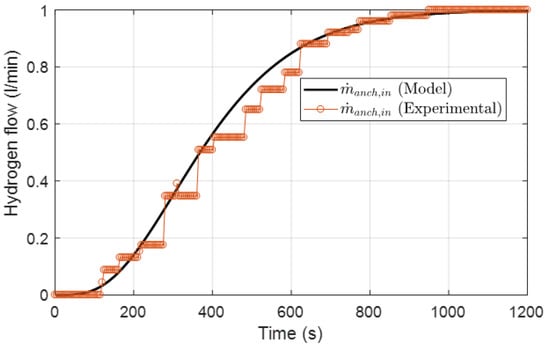
Figure 4.
Response of the reformer output to a step change as a 4th order overdamped system compared against experimental data.
2.2. Model for the HT-PEMFC
A semi-empirical nonlinear mathematical model was developed that considers its main variables to be the partial pressures of all gases, the fuel cell current, and the operating temperature. This model is an extension of the detailed mathematical model presented in [20]. The main difference is that the original model was for an LT-PEMFC, whereas this work deals with the operation of an HT-PEMFC. To adapt the original model to the HT-PEMFC model, two important modifications were implemented. First, water management is not considered in this model’s mass balances. Because of the fuel cell’s high temperature, water does not exist in a liquid form but a vapor form. The second modification refers to the electrochemical parameters of the I–V curve that were adapted to fit the desired trajectory of the curve. An experimental study was performed to validate the behavior of the model when applied to an HT-PEMFC.
The model accounts for mass balance dynamics in the gas flow channels (anode, cathode), the gas diffusion layers (GDL), and the membrane as follows:
where , are the species masses (oxygen, nitrogen, water vapor) in the cathode channel, , are the input mass flows of the species in the channel, while are the output mass flows of the species in the channel, are the oxygen and vapor molar masses, is the membrane active area, is the fuel cell’s current and is the Faraday number.
The rate of evaporation inside the cathode channel is expressed by:
where is the saturation pressure of water defined at the operation temperature of the fuel, is the vapor pressure inside the cathode channel, is the cathode channel volume, is the evaporation rate, is the gas constant and is the operational temperature of the fuel cell.
The partial pressure of water vapor in each side of the gas diffusion layers (anode, cathode) satisfies the respective mass balance Equation:
where is the vapor molar flux that diffuses from the anode channel to the GDL, is the vapor molar flux that diffuses from the cathode channel to the GDL, is the overall vapor molar flow across the membrane, and is the diffusion channel thickness. The overall mass flow rate of the vapor that passes through the membrane is calculated by:
The performance of a fuel cell is shown by a graph of its output voltage versus the drawn current density. This graph, which is also referred to as the polarization curve, contains some of the most important characteristics of a fuel cell. To determine this relationship, the cell voltage is defined as the difference between the ideal Nernst voltage and several voltage losses. These losses increase as the current drawn from the fuel cell increases. At low current densities, the activation losses appear due to the slowness of the reactions taking place on the surface of the electrodes. As the current density increases, ohmic losses appear across the proton exchange membrane caused by the resistance of the membrane to the hydrogen ions transporting through it. Finally, at high current densities the concentration losses are significantly affected due to the consumption of the reactants at greater rates than they can be supplied, while the product accumulates at a greater rate than it can be removed. The equation that takes into consideration the above losses is:
The values of the empirical parameters are shown in Table 2.
Table 2.
Electrochemical Parameters.
2.3. Model for the Li-Ion Battery
In this work, the kinetic battery model (KiBaM) is used [21] which was originally developed for lead-acid batteries but can also be used for lithium-ion batteries with sufficient accuracy.
In this model, the battery charge is distributed over two wells: the available-charge well , and the bound-charge well, , as seen in Figure 5. The available-charge well supplies electrons directly to the load, whereas the bound-charge well supplies electrons only to the available-charge well. The rate at which charge flows between the wells depends on the difference in height of the two wells, and on a parameter . The parameter gives the fraction of the total charge in the battery that is part of the available-charge well. The equations that describe the model are given as follows:

Figure 5.
Kinetic battery model.
The algebraic equations that determine the operating voltage, the available power, and the state of charge (SOC) are described below:
Charge case
where is the internal voltage, is the internal resistance, and are the operating current and voltage, respectively, and is the charging power. The value of the internal voltage is given by Equation (22):
where is the maximum allowed internal charging voltage and is the minimum allowed internal charging voltage.
Discharge case
where is the internal voltage, is the operating voltage and is the discharging power. The value of the internal voltage is given by Equation (25):
where is the minimum allowed internal discharging voltage and is the maximum allowed internal discharging voltage.
Finally, the state of charge of the accumulator is defined as the available fraction of power at each time instance:
2.3.1. Experimental Validation of the HT-PEMFC Model
In this section, to validate the accuracy of the derived model, a comparison against experimental is performed. Both steady-state validation and dynamic validation of the model were conducted. The polarization curve of the fuel cell derives from two indicative sets of experiments at 105 Pa pressure and 180 °C temperature. All experiments were conducted at the test unit in CPERI/CERTH.
Figure 6 illustrates a comparison between the model predictions of the cell stack against experimental data from the unit. The dashed lines depict the 95% confidence intervals of the conducted experiments. A good agreement is achieved throughout the range of the current density values since the model predictions are within the confidence region. Figure 7 and Figure 8 depict the dynamic response of voltage and power, respectively. In both figures, the step changes in the current are imposed on the fuel cell model and the result is the model’s voltage or power. The comparison of the experimental data and the model’s predictions shows good agreement for both variables (voltage, power). Looking at both the static and dynamic validation, the conclusion is a clear indication that the model has the required accuracy to describe the behavior of the system.
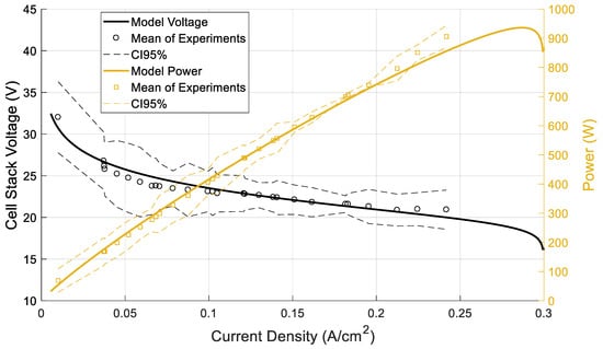
Figure 6.
Steady-state response of HT-PEMFC model.
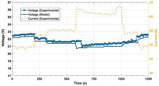
Figure 7.
Dynamic voltage response of the HT-PEMFC model to current step changes.

Figure 8.
Dynamic power response of the HT-PEMFC model to current step changes.
2.3.2. Experimental Validation of Li-Ion Battery Model
In this section, to validate the accuracy of the model, a comparison between experimental data and the model predictions is conducted. Two indicative sets of experiments are presented to demonstrate the accuracy of the model, one regarding a charging cycle with a constant current at 10 A and one regarding a discharging cycle with a constant current at 40 A.
Figure 9 and Figure 10 illustrate a comparison between the model prediction for the voltage of the Li-ion battery and experimental data regarding charging and discharging, respectively. A full cycle (0–100% and 100–0% SOC) is shown in both figures. The dashed lines depict the 95% confidence intervals of the conducted experiments. A good agreement is achieved throughout the linear part of the experimental data since the model predictions are within the confidence region. The beginning and the end of this linear part mark the capacity limits under nominal operation, ranging from 20% minimum capacity (24 Ah) to 80% maximum capacity (96 Ah). The error which is observed outside the minimum and maximum capacity range does not affect the model’s accuracy since it is beyond the operating limits of the system. Throughout the rest of the capacity range, a negligible error exists between the model prediction and the real operation of the battery. The root-mean-square error (RMSE) was 0.344 V in the charging cycle and 0.213 V in the discharging cycle. The above metric was calculated using 7200 samples over a period of 10 h with a 5 s interval and 1800 samples over a period of 2.5 h with a 5 s interval for the charging and discharging case, respectively. This measure is a clear indication that the model has the required accuracy to describe the behavior of the system.
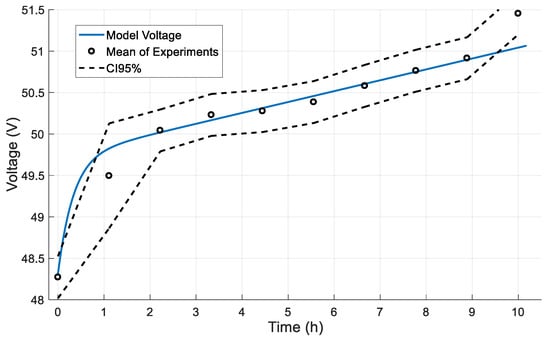
Figure 9.
Dynamic response in a full charge cycle.
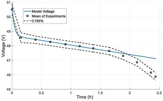
Figure 10.
Dynamic response in a full discharge cycle.
The beginning and the end of this linear part mark the capacity limits under nominal operation, ranging from 20% minimum capacity (24 Ah) to 80% maximum capacity (96 Ah). In the exponential areas (outside of the min–max capacity range) an increasing error is observed due to the linear behavior of the model. This error does not affect the model’s accuracy since it is present only outside of the operational limits of the battery.
3. Control System Design
In this section, the model-based control framework of the integrated system is presented. This includes a presentation of the control objectives, as well as a mathematical representation of the NMPC framework and the optimization procedure.
3.1. Control Objectives and Input–Output Structure
The control objectives for the system are to generate the required power while maintaining the operation in a safe region. The variable power demand is achieved by manipulating the current which is applied to the fuel cell by the converter connected to the system. The safe operation is maintained by controlling the reactants at a certain excess ratio level to avoid starvation by manipulating the air and hydrogen flows . The safe operating region is defined by the oxygen and hydrogen excess ratios , expressed as the ratios of the input flow of each gas to the consumed quantities per unit time due to the reaction [22,23,24].
where, are the oxygen and hydrogen input flows at the channels, whereas are the respective reacted quantities. The input flow of hydrogen to the anode channel of the fuel cell originates from the reformer. When the NMPC controller assigns a new target value for , this manipulated variable cannot acquire this value instantly because of the reformer’s time delay. Therefore, the reformer imposes its delay to the hydrogen entering the anode resulting in the dynamic behavior of . Additionally, the controller aims to maintain the battery cells’ SOC at a certain level, which is achieved by manipulating the battery current . These objectives are accomplished by the control configuration which is depicted in Figure 11.
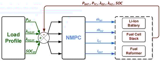
Figure 11.
Control configuration and information/signal flow between the nonlinear model predictive control (NMPC) and the integrated unit including the error calculation.
As and SOC are unmeasured variables, they are estimated by the nonlinear models for the fuel cell and the battery. Based on the control configuration shown in Figure 11, a constant set-point regarding the excess ratios of hydrogen, oxygen, and the battery state of charge is used.
3.2. Nonlinear Model Predictive Control Framework
Nonlinear model predictive control is part of a family of optimization-based control methods which calculate the optimal values of the future control moves using model prediction over a future time horizon [25]. The control actions minimize a cost function related to control objectives of the system subject to a nonlinear dynamic model. The optimization yields an optimal control sequence over a control horizon and only the first control action for the current time interval is applied to the system. At the next time interval, the horizon is shifted by one sampling interval and the optimization problem is resolved using the information of the new measurements acquired from the system [25]. The mathematical representation of the NMPC algorithm is [26,27]:
subject to:
The minimization of functional J (Equation (29)) is subject to constraints on the manipulated and controlled variables (Equation (35)). The variable denotes the desired reference trajectory, represents the differential equations and represents the algebraic equations of the output variables. In this application, is the desired power profile where we assume that this system is used as a portable small-scale power generation station. The difference between the measured variable and the corresponding predicted value at time instance is assumed to be constant for the entire length of the prediction horizon , denotes the control horizon reached through time intervals. Tuning parameters of the algorithm are the weight factors in the objective function and the length of the prediction and control horizon that reflect on the relative importance of the control objectives.
In the last decade, considerable progress has been achieved towards the solution of challenging dilemmas [28] that has enabled the wider application of the NMPC framework. The computational progress of the optimization algorithms allows for both decreases in computational delays and minimization of the approximation errors. Recently, NMPC controllers have been based on nonlinear programming (NLP) sensitivity with reduced computational costs and can lead to significantly improved performance [29]. Overall, the application of dynamic optimization in conjunction with fast optimization solvers allows the use of first-principles models for NMPC [30]. In general, a differential-algebraic equation constrained optimization problem is considered, which includes the continuous-time counterpart of the NMPC problem. Since the implemented NMPC algorithm involves inequality constraints, direct optimization methods are used for the optimization problem which is transformed into an NLP problem.
3.3. Prediction Horizon
One of the main characteristics of NMPC is that it can anticipate future events and can adjust the control actions accordingly in a feed-forward fashion in order to obtain a prediction horizon length that can provide effective control and reasonable computational effort. In Table 3, a metric is shown in an analysis of different prediction horizon intervals. It represents the root-mean-square error (RMSE), which is presented for the power profile set point and the two excess ratios set points (hydrogen and air). The RMSE for the power profile is calculated between the power profile set point and the summation of power from the fuel cell and battery .
Table 3.
Prediction horizon analysis.
An important aspect of the NMPC control algorithm—as implemented in this study—is the resulting behavior of the subsystems. In this case, this is mainly the fuel cell and the battery. Rapid fluctuations in the power demand are preferably met by the battery component due to its faster response to prevent the fuel cell from degrading. The fuel cell exhibits much slower dynamics and the maintenance of a specific operating level is crucial for the health of the component. Improved efficiency is also the reason why the battery should be deployed to satisfy high peaks in the load demand.
Figure 12 shows a comparison between four different prediction horizon lengths (one, two, three, and five intervals) and their resulting power distribution among the fuel cell and battery. Each interval represents 1 min of real-time operation. For the specific application where the reformer integrated into the system exhibits a time delay of approximately 2 min to reach a steady-state, and considering that the reformer is the major dynamic component of the system, we decided that a 1 min time interval offers a sufficient accuracy and decent computational burden in order to capture this dynamic. In all four cases, the battery delivers power when it is instantly needed. However, the fuel cell shows an oscillatory behavior in Figure 12a. The smoothest curve regarding fuel cell power is the one that corresponds to a prediction horizon of two intervals. Although Figure 12c,d shows good results, these are accompanied by an increase in computational time. Since computational time is heavily hardware-dependent, it can be neglected if a high-end computer is used, that is why it is not considered as a metric in this study.
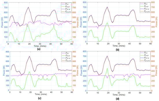
Figure 12.
Comparison of different prediction horizon values: (a) 1 interval; (b) 2 intervals; (c) 3 intervals; (d) 5 intervals.
Generally, larger prediction horizons result in worse behavior because then the model’s predictions are increasingly susceptible to future disturbances. On the other hand, the smaller the horizon is the higher the oscillations that the model prediction will introduce. A highly oscillatory behavior is not desired for a fuel cell, which means that a tradeoff between prediction accuracy and smoothness of the curve is necessary. After exploring both aspects (metric and behavior) for the selection of an appropriate value the conclusion is that the smallest possible prediction horizon with acceptable accuracy is desired. Therefore, the prediction horizon for this study is set to two intervals.
4. Operation Scenarios and Results
This section presents selected operation scenarios and their results obtained from the application of the NMPC controller using the nonlinear models developed in Section 2. The behavior of the integrated system is exemplified here by two case studies. In the first one, the fuel cell and battery operate as two individual power sources, satisfying the power demand, and no charging of the battery is considered. In the second case study, the demand is satisfied the same way as in the first case and the battery is also charged by the fuel cell.
The objective function of each case is formulated in such a way that the power set-point is reached, and the operating restrictions are satisfied. Both cases have some common points referring to the implementation of the NMPC. The scenarios into consideration show the operation and response of each subsystem for a period of 1 h. The control horizon is 1 interval for both cases. The amount of time chosen for is enough time for the battery and the fuel cell to reach a steady state. Additionally, the constraints were chosen so that throughout the operation, the integrated system is always within the limits of safe operation.
4.1. Power Demand Satisfaction by the Battery and the Fuel Cell
In this case study, the fuel cell and the battery satisfy the power demand as two individual power sources. Battery charging is not considered.
4.1.1. Objective Function
The purpose of the objective function is, on one hand, the power demand satisfaction and on the other hand the operation of the fuel cell at specific hydrogen and oxygen excess ratios that were set as set-points.
subject to:
The variable represents the power provided by the battery to the load demand. adds up with to result in the total dedicated power to reach the setpoint . Variables and are the manipulated variables that govern the power output of the battery and the fuel cell accordingly. Furthermore, in order to balance the excess ratios of hydrogen and air and maintain them within the specified limits, the other two manipulated variables and are employed to control the mass flows of the two species. The operation of the battery is supervised by its state of charge that has an upper limit to avoid overcharging and a lower limit to avoid depletion. The first quadratic term of the objective function represents the tracking of the power profile with the error estimation between the process and the model incorporated as well. The other two terms represent the effort to maintain the fuel cell operation at the desired levels to avoid hydrogen and oxygen starvation at the anode and cathode, respectively.
4.1.2. Simulation Scenario and Discussion of Results
To evaluate the operation of the integrated unit and the response of the NMPC framework, the behavior of each subsystem, the manipulated variables, and the controlled variables are presented, along with the analysis of main variables representing the operational state, such as the battery voltage. The following figures show the results of the simulation for the optimal control of the fuel cell with the reformer and the battery.
In Figure 13, the fuel cell provides an almost constant power as a result of its slower dynamics (because of the slow dynamic of the reformer). On the other hand, the battery, with its faster response time, supplies the demanded power during rapid changes. The provided power by the battery and the fuel cell shows that the reference power trajectory is followed regardless of the changes. Therefore, the system accomplishes its main target.
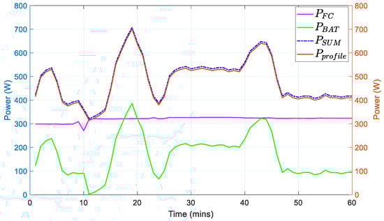
Figure 13.
Fuel cell and battery power in reference to the power profile.
The behavior of the manipulated variables in Figure 14 is shown. The battery current follows the trajectory of the power profile whereas the fuel cell current and the air flow from the compressor maintains almost a constant value. The hydrogen flow coming from the reformer increases gradually by 1 l/min starting at the 10 min mark due to the time delay forced by the reformer. Figure 15 verifies that the operation of the fuel cell remains within the predefined operation constraints for the hydrogen and oxygen ratios throughout the scenario.
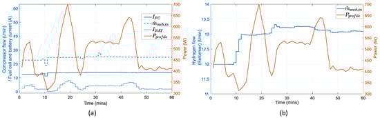
Figure 14.
Manipulated variables in reference to the power profile: (a) input air flow entering the anode channel, fuel cell current, and battery current; (b) output hydrogen flow of the reformer entering the anode channel.
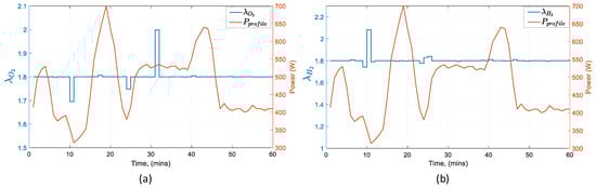
Figure 15.
Fuel cell operating set-points in reference to the power profile: (a) oxygen excess ratio, (b) hydrogen excess ratio.
To evaluate the behavior of the battery, two important variables are shown, the voltage and the state of charge. Figure 16 (left) shows that when the battery supplies more power, the voltage drop is increased. The slope of the state of charge is proportional to the rate of discharge Figure 16 (right), which is steeper when the power increases.
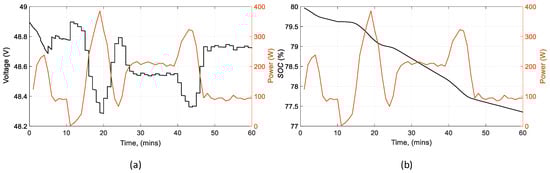
Figure 16.
Battery parameters in reference to its power: (a) battery voltage (b) battery state of charge.
4.2. Fuel Cell Satisfies Power Demand and Charges the Battery
In this case study, the two devices operate to satisfy the power demand and also maintain the battery state of charge at a certain desired level by charging it. To achieve this, the fuel cell must provide the demanded power by the load and the power needed to charge the battery. An important feature of this formulation is that the battery can only operate in one mode, charging or discharging. This leads to the addition of two Boolean variables that transform the problem from NLP to mixed-integer nonlinear programming (MINLP).
4.2.1. Objective Function
The charging power of the battery comes from the fuel cell. Therefore, the term is added to so that the charging power increases the fuel cell’s set point. The charging power was chosen arbitrarily at 100 W. The term represents the same thing as in the previous case study; that is, the power the battery provides to the load. The last term of the objective function establishes a goal for the system; that is, to reach the desired state of charge set point . The additional constraint containing the two Boolean variables ensures that their value is either zero or one and that they can never have the same value. This translates to the ability of the battery to either be charged or discharged and never execute both.
subject to:
4.2.2. Simulation Scenario and Discussion of Results
A different power profile is implemented with constant power demand areas and fewer fluctuations. The prediction and control horizon were set at one interval each, which was the smallest possible value with acceptable accuracy.
Figure 17 illustrates the integrated system’s response. At the beginning of the simulation, the fuel cell starts operating at a level way lower than what is required from the load profile. The battery takes on to cover this difference until the slow response of the reformer allows enough hydrogen to flow to the fuel cell in order to produce the required power. Charging is achieved between 15 to 33 min into the process (negative battery power values). This area of the power profile allows charging to occur because the fuel cell’s power is already at a high level and can cover the power demand and also supply the rest of its power to the battery. When the demand increases again, the fuel cell can no longer sustain the charging of the battery and dedicates its whole capacity to satisfy the power demand.
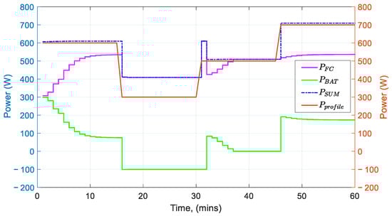
Figure 17.
Fuel cell and battery power in reference to the power profile.
In Figure 18, the manipulated variables and, in particular, the fuel cell current and the air flow from the compressor, follow a trajectory similar to that of the . The battery current follows the battery’s power curve, except for the part where it is charging. During that part, the current is dictated by the battery voltage and is calculated to account for a charging power of . The hydrogen flow depicts the response of the reformer. The reformer determines how fast the fuel cell delivers the required power.
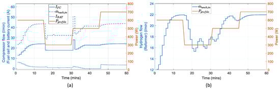
Figure 18.
Manipulated variables in reference to the power profile: (a) input air flow entering the anode channel, fuel cell current, and battery current; (b) output hydrogen flow of the reformer entering the anode channel.
Figure 19 determines whether the fuel cell operates in the safe region or not. The excess ratio of air is almost constant and equal to the set-point throughout the simulation. The excess ratio of hydrogen changes rapidly when the power demand changes at the next time interval. This occurs due to the reformer’s inability to transfer less hydrogen instantly to the fuel cell when the demand is lower and therefore, the ratio increases. The exact opposite occurs when the demand is higher. In Figure 20, the battery state of charge decreases during discharging with different rates according to the battery current. When the battery is charging, between 15 to 33 min, SOC increases, again, with different rates depending on the current of the battery.
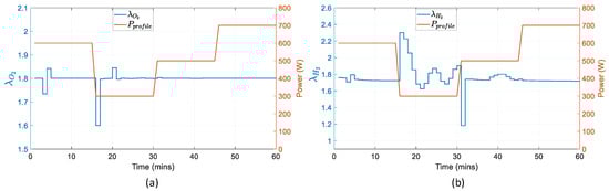
Figure 19.
Fuel cell operating set-points in reference to the power profile: (a) oxygen excess ratio; (b) hydrogen excess ratio.
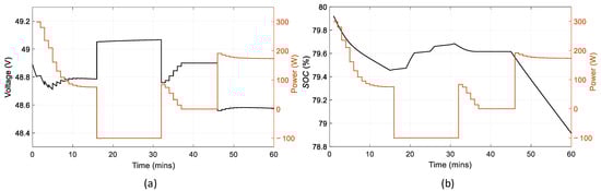
Figure 20.
Battery parameters in reference to its power: (a) battery voltage; (b) battery state of charge.
5. Conclusions
In this work, an advanced multivariable NMPC control framework was developed for an integrated LPG reforming-HT-PEM fuel cell and Li-ion accumulator system. The nonlinear continuous dynamic models used for this work were tested and experimentally validated to best fit the existing power unit. A set of case studies, in which the performance and reliability of the controller were simulated, were proposed and implemented. In each case, the safe operation of the fuel cell and the accumulator was ensured through a constrained optimization methodology. Furthermore, the case studies indicate that the illustrated system can adjust to set-point changes of the load demand. Overall, the proposed approach guarantees that the HT-PEMFC performs within its operating limits and illustrates an excellent potential for on-line applications in order to manage the produced energy in an optimum manner.
Author Contributions
Conceptualization, A.K., C.Z., S.P., S.V. and P.S.; data curation, A.K. and C.Z.; formal analysis, A.K., C.Z., S.P., S.V. and P.S.; investigation, A.K., C.Z., S.P., S.V. and P.S.; methodology, A.K., C.Z. and S.P.; resources, C.Z., S.P., S.V. and P.S.; software, A.K. and C.Z.; supervision, C.Z., S.P., S.V. and P.S.; validation, A.K., C.Z. and S.P.; visualization, C.Z., S.P., S.V. and P.S.; Writing—Original draft, A.K. and C.Z.; Writing—Review and editing, A.K., C.Z., S.P. and P.S. All authors have read and agreed to the published version of the manuscript.
Funding
This research received no external funding.
Institutional Review Board Statement
Not applicable.
Informed Consent Statement
Not applicable.
Data Availability Statement
Not applicable.
Conflicts of Interest
The authors declare no conflict of interest.
References
- Wang, J.; Wang, H.; Fan, Y. Techno-Economic Challenges of Fuel Cell Commercialization. Engineering 2018, 4, 352–360. [Google Scholar] [CrossRef]
- Scott, K.; Pilditch, S.; Mamlouk, M. Modelling and experimental validation of a high temperature polymer electrolyte fuel cell. J. Appl. Electrochem. 2007, 37, 1245–1259. [Google Scholar] [CrossRef]
- Ziogou, C.; Voutetakis, S.; Georgiadis, M.C.; Papadopoulou, S. Model predictive control (MPC) strategies for PEM fuel cell systems—A comparative experimental demonstration. Chem. Eng. Res. Des. 2018, 131, 656–670. [Google Scholar] [CrossRef]
- Barzegari, M.M.; Alizadeh, E.; Khorshidian, M.; Rahgoshay, S.M.; Saadat, S.H.M. Nonlinear Grey-Box Modeling and Model Predictive Control for Cascade-Type PEM Fuel Cell Stack. In Proceedings of the 2017 IEEE Vehicle Power and Propulsion Conference, VPPC 2017-Proceedings, Belfort, France, 11–14 December 2017; Institute of Electrical and Electronics Engineers Inc.: New York, NY, USA, 2018; pp. 1–5. [Google Scholar]
- Luna, J.; Jemei, S.; Yousfi-Steiner, N.; Husar, A.; Serra, M.; Hissel, D. Nonlinear predictive control for durability enhancement and efficiency improvement in a fuel cell power system. J. Power Sources 2016, 328, 250–261. [Google Scholar] [CrossRef]
- Luna, J.; Usai, E.; Husar, A.; Serra, M. Enhancing the efficiency and lifetime of a proton exchange membrane fuel cell using nonlinear model-predictive control with nonlinear observation. IEEE Trans. Ind. Electron. 2017, 64, 6649–6659. [Google Scholar] [CrossRef]
- Hähnel, C.; Aul, V.; Horn, J. Power Control for Efficient Operation of a PEM Fuel Cell System by Nonlinear Model Predictive Control. IFAC Pap. 2015, 48, 174–179. [Google Scholar] [CrossRef]
- Schultze, M.; Horn, J. Modeling, state estimation and nonlinear model predictive control of cathode exhaust gas mass flow for PEM fuel cells. Control Eng. Pract. 2016, 49, 76–86. [Google Scholar] [CrossRef]
- Hong, L.; Chen, J.; Liu, Z.; Huang, L.; Wu, Z. A nonlinear control strategy for fuel delivery in PEM fuel cells considering nitrogen permeation. Int. J. Hydrogen Energy 2017, 42, 1565–1576. [Google Scholar] [CrossRef]
- Ouyang, Q.; Chen, J.; Wang, F.; Su, H. Nonlinear MPC Controller Design for AIR Supply of PEM Fuel Cell Based Power Systems. Asian J. Control 2017, 19, 929–940. [Google Scholar] [CrossRef]
- Najafi, B.; Mamaghani, A.H.; Rinaldi, F.; Casalegno, A. Fuel partialization and power/heat shifting strategies applied to a 30 kWel high temperature PEM fuel cell based residential micro cogeneration plant. Int. J. Hydrogen Energy 2015, 40, 14224–14234. [Google Scholar] [CrossRef]
- Mamaghani, A.H.; Najafi, B.; Casalegno, A.; Rinaldi, F. Long-term economic analysis and optimization of an HT-PEM fuel cell based micro combined heat and power plant. Appl. Therm. Eng. 2016, 99, 1201–1211. [Google Scholar] [CrossRef]
- Mamaghani, A.H.; Najafi, B.; Casalegno, A.; Rinaldi, F. Predictive modelling and adaptive long-term performance optimization of an HT-PEM fuel cell based micro combined heat and power (CHP) plant. Appl. Energy 2017, 192, 519–529. [Google Scholar] [CrossRef]
- Mamaghani, A.H.; Najafi, B.; Casalegno, A.; Rinaldi, F. Optimization of an HT-PEM fuel cell based residential micro combined heat and power system: A multi-objective approach. J. Clean. Prod. 2018, 180, 126–138. [Google Scholar] [CrossRef]
- Najafi, B.; Mamaghani, A.H.; Baricci, A.; Rinaldi, F.; Casalegno, A. Mathematical modelling and parametric study on a 30 kWel high temperature PEM fuel cell based residential micro cogeneration plant. Int. J. Hydrogen Energy 2015, 40, 1569–1583. [Google Scholar] [CrossRef]
- Ipsakis, D.; Voutetakis, S.; Papadopoulou, S.; Seferlis, P. Optimal operability by design in a methanol reforming-PEM fuel cell autonomous power system. Int. J. Hydrogen Energy 2012, 37, 16697–16710. [Google Scholar] [CrossRef]
- Ipsakis, D.; Ouzounidou, M.; Papadopoulou, S.; Seferlis, P.; Voutetakis, S. Dynamic modeling and control analysis of a methanol autothermal reforming and PEM fuel cell power system. Appl. Energy 2017, 208, 703–718. [Google Scholar] [CrossRef]
- Ziogou, C.; Giaouris, D.; Papadopoulou, S.; Voutetakis, S. Integrated design and operation assessment of an embedded supervisory automation framework for a hybrid hydrogen-enabled power generation system. Comput. Aided Chem. Eng. 2016, 38, 1359–1364. [Google Scholar]
- Technology-Helbio. Available online: https://helbio.com/technology/ (accessed on 18 July 2019).
- Ziogou, C.; Voutetakis, S.; Papadopoulou, S.; Georgiadis, M.C. Modeling, Simulation and Validation of a PEM Fuel Cell System. Comput. Chem. Eng. 2011, 35, 1886–1900. [Google Scholar] [CrossRef]
- Manwell, J.F.; McGowan, J.G. Lead Acid Battery Storage Model for Hybrid Energy Systems. Sol. Energy 1993, 50, 399–405. [Google Scholar] [CrossRef]
- Arce, A.; del Real, A.J.; Bordons, C.; Ramirez, D.R. Real-Time Implementation of a Constrained MPC for Efficient Airflow Control in a PEM Fuel Cell. IEEE Trans. Ind. Electron. 2010, 57, 1892–1905. [Google Scholar] [CrossRef]
- Vahidi, A.; Stefanopoulou, A.; Peng, H. Current Management in a Hybrid Fuel Cell Power System: A Model-Predictive Control Approach. IEEE Trans. Control Syst. Technol. 2006, 14, 1047–1057. [Google Scholar] [CrossRef]
- Chen, H.; Allgöwer, F. A Quasi-Infinite Horizon Nonlinear Model Predictive Control Scheme with Guaranteed Stability. Automatica 1998, 10, 1205–1217. [Google Scholar] [CrossRef]
- Qin, S.; Badgwell, T. A survey of industrial model predictive control technology. Control Eng. Pract. 2003, 11, 733–764. [Google Scholar] [CrossRef]
- Allgöwer, F.; Findeisen, R.; Nagy, Z.K. Nonlinear Model Predictive Control: From Theory to Application. J. Chin. Inst. Chem. Eng. 2004, 35, 299–315. [Google Scholar]
- Mayne, D.Q.; Rawlings, J.B.; Rao, C.V.; Scokaert, P.O.M. Constrained model predictive control: Stability and optimality. Automatica 2000, 36, 789–814. [Google Scholar] [CrossRef]
- Diehl, M.; Bock, H.; Schloder, J.; Findeisen, R.; Nagy, Z.; Allgöwer, F. Real-time optimization and nonlinear model predictive control of processes governed by differential-algebraic equations. J. Process Control 2002, 12, 577–585. [Google Scholar] [CrossRef]
- Zavala, V.M.; Biegler, L.T. The Advanced Step NMPC Controller: Optimality, Stability and Robustness. Automatica 2009, 45, 86–93. [Google Scholar] [CrossRef]
- Diehl, M.; Ferreau, H.J.; Haverbeke, N. Efficient numerical methods for Nonlinear MPC and Moving Horizon Estimation. In Nonlinear Model Predictive Control; Springer: Berlin/Heidelberg, Germany, 2009; pp. 391–417. [Google Scholar]
Publisher’s Note: MDPI stays neutral with regard to jurisdictional claims in published maps and institutional affiliations. |
© 2021 by the authors. Licensee MDPI, Basel, Switzerland. This article is an open access article distributed under the terms and conditions of the Creative Commons Attribution (CC BY) license (http://creativecommons.org/licenses/by/4.0/).