Probabilistic Modeling and Equilibrium Optimizer Solving for Energy Management of Renewable Micro-Grids Incorporating Storage Devices

Abstract

Recently, micro-grids (MGs) have had a great impact on power system issues due to their clear environmental and economic advantages. This paper proposes an equilibrium optimizer (EO) technique for solving the energy management problem of MGs incorporating energy storage devices concerning the emissions from renewable energy sources (RES) of MGs. Because of the imprecision and uncertainties related to the RESs, market prices, and forecast load demand, the optimization problem is described in a probabilistic manner using a 2m + 1 point estimation approach. Then, the EO approach is utilized for solving the probabilistic energy management (EM) problem. The EM problem is described according to the market policy on the basis of minimizing the total operating cost and emission from RESs through optimal settings of the power generated from distributed generators (DGs) and grids connected under the condition of satisfying the operational constraints of the system. The proposed EO is evaluated based on a grid-connected MG that includes energy storage devices. Moreover, to prove the effectiveness of the EO, it is compared with other recently meta-heuristic techniques. The simulation results show acceptable robustness of the EO for solving the EM problem as compared to other techniques.

1. Introduction

The exponential increase in universal power demand has had a major impact on the rapid depletion of fossil fuels, which has resulted in increasing gas emissions from conventional generators. To solve this problem, the world has tended to encourage obtaining energy from renewable energy resources (RESs) such as wind turbines (WT), photovoltaics (PV), biomass, fuel cell (FC), micro-turbines (MT), hydropower, tides, and energy storage (ES) devices [1,2]. It is worth noting that micro-grids (MGs) systems have an important vital role in solving different energy-related problems such as reducing the minimization of the operating costs, transmission losses, environmental pollution, and peak load as well as improving voltage regulation and participating in frequency regulation. The MGs systems consist of different technologies of non-dispatchable and dispatchable renewable energy sources (RES), ES devices, and dispatchable loads. Further, MGs enable the active sharing of customers by giving them real-time control and access to the information [3,4,5].

Considering all mentioned benefits, more and more extra small MGs have been deployed over all the world such as facilities, military bases, hospitals, and industries in recent ten years [6]. With the high penetration of energy from RESs in the existing power systems, it also has the important impact of reducing energy losses, pollutant emissions, and enhancing power system performance. However, the improper utilization of RESs leads to problems in the operation of the system [7,8].

Generally, MGs may operate in islanding mode or interconnected to the main grid, in which the energy can be bought from or sold to the grid or be isolated from the grid as a controlled entity [1,9]. The energy management (EM) problem has a complex and nonlinear nature problem. However, managing MG sources for minimizing the total operating cost depends on a precise model with the consideration of multiple objectives and achieving different operational constraints such as power limit of the various DGs sources, power balance equations, and spinning reserve. Due to pollutant emissions from the generating units, the minimization of emissions can be furthermore included in the EM problem as an objective function. Obtaining efficient EM is the main task in the optimization process. Therefore, an intelligent technique is required to obtain the optimal operation of the MGs for achieving the concerned objectives.

There are two general methods of representing the EM problem, namely, the deterministic and probabilistic methods. These methods are objectively applied for solving the EM problems [7,10]. In the deterministic methods, the demand load, output power of RES, and market prices are fixed at their expected value without considering the factors of change and uncertainty. However, the uncertainties may be associated with those input variables.

The traditional EM problem is described as a deterministic EM based on the concept that the network parameters and input variables are precisely known. In other words, it is assumed that the network parameters, the output power produced from DG units, and load demands are known deterministic. Therefore, the deterministic EM techniques are extremely dependent on the accuracy of input variables. However, numerous random disturbances have occurred in the distribution network operations such as the change in power network configuration, the market price, the variation of load, and the stochastic nature of the produced power of the DG units as the PV and WT units. Accordingly, these randomly occurring factors are the main source of the uncertainty. Therefore, it is necessary to integrate these uncertainties inherent in describing the load, output from RES, and market prices in a probabilistic manner during EM modeling to overcome the inaccuracy in the results of the EM.

Recently, many researchers have been interested in solving both deterministic and probabilistic EM problems by proposing efficient techniques for obtaining the optimal solution. The multi-objective particle swarm optimization (MOPSO) algorithm was proposed in [11] to find the optimal scheduling of generation units within MG’s through analyzing the exchange power between MGs and the main grid, also considering the demand-side management (DSM). Based on a novel parallel hybrid genetic algorithm (GA) with particle swarm optimization (PSO), the developed efficient algorithm was proposed in [12] for solving both sizing and EM optimization problems. The authors suggested in [13] a two-stage robust optimization model incorporating the resiliency of the microgrid through supporting islanding events without curtailment of load, along with ensuring the robustness versus the uncertainties of RESs. Output powers of PV panels, fuel cell, and the ES device are integrated based on a multi-winding magnetic coupled link for supplying a residential load as implemented in [14] to solve EM concerning grid-connected and islanding operation modes of MG.

Due to the uncertainty of RESs and demand load, the authors in [15] proposed an economic model of MG connected to the main grid with the consideration of ES lifetime for achieving the reliability and safety of the proposed system. Considering the uncertainties of solar irradiance, wind speed, and demand load, the nondominated sorting genetic algorithm (NSGAII) was utilized for optimal operation of the MG for an islanding mode [16] and for a grid-connected mode [17]. For minimizing the total generating cost of the EM problem based on the energy scheduling of MG, the authors in [18] utilized a multi-layer ant colony optimization (MACRO) approach. In [19], a multi-period artificial bee colony (MABC) optimization was proposed for solving the economic dispatch (ED) problem, considering the ES devices and responsive load bids. In [20], an imperialist competitive algorithm (ICA) was applied on the MG in interconnected mode to minimize the operating cost, considering output power and load uncertainties, where the obtained results were compared with Monte Carlo simulation techniques. The work presented in [21] showed the energy investments in MG including different technologies of RES at the distribution system, where the joint investment and operation were modeled as a two-period of the developed stochastic program.

The probabilistic technique based on the two-point-estimate method for solving the EM problem using GA was proposed in [22] for minimizing the operating cost of a system that includes ES devices and controllable loads. An efficient optimization algorithm of PSO for computing the optimal EM solution with different DG units and ES devices was developed in [23], where the EM problem was solved in a probabilistic manner. To solve the EM problem, a gravitational search algorithm (GSA) with the 2m point estimate technique was employed in [24], considering the uncertainties of MG sources. Additionally, the 2m + 1 point estimation technique with a self-adaptive charged system search (SACS) algorithm [25] and a modified firefly optimization algorithm (MFA) [26] have been employed for solving the probabilistic EM problem, considering the uncertainties of load demand, sources of MG, and load demand. The efficient salp swarm algorithm (ESSA) along with the 2m + 1 point estimation technique has been developed in [8] to solve the EM probabilistic problem by considering the pollutant emission from the RES.

Equilibrium Optimizer (EO) is a novel physics-based optimization algorithm recently published in 2020 [27]. However, EO can solve the various optimization problems successfully. As proposed in [28], the economic dispatch (ED) problem was solved by minimizing the total fuel cost, considering the active power constraint, effect of valve point, loss of transmission line, and the limits of ramp rate. In addition, the EO was employed in [29] for extracting the best values of undefined parameters for the developed mathematical model of the proton exchange membrane fuel cell (PEMFC).

In this paper, the EO is proposed for solving both deterministic and probabilistic EM problems by considering the pollutant emission of MG sources and including ES devices. Moreover, the 2m + 1 point estimation technique is used to represent the sources that have uncertainties in the MGs. Where, the random variation of input variables is expressed in terms of Weibull probability density function. After that, EO is applied for each case resulting from 2m + 1 technique. Finally, the Gram-Charlier expansion method is utilized for obtaining the probability distribution of random variables output results based on the EO algorithm. Here, the optimization of EM problem is formulated including two various objective functions for minimizing both the total operating cost of MG sources with ES devices and emission from RESs. However, the objective function is modeled as a single objective function by using a price penalty function and weighting factors instead of modeled as a multi-objective function. Then, the proposed EO is tested and compared with other recent algorithms using a standard model of grid-connected MG through different scenarios. The contributions of this paper are to:

• Formulate the optimization problem of EM incorporating ES devices with consideration of the emissions from RESs via converting the multi-objective function problem into a coefficient single objective function using a price penalty factor and weighting factors by handling the operational constraints.
• Model the uncertainties of RESs with ES devices, demand load, and market prices, then apply (2m + 1) point estimate method.
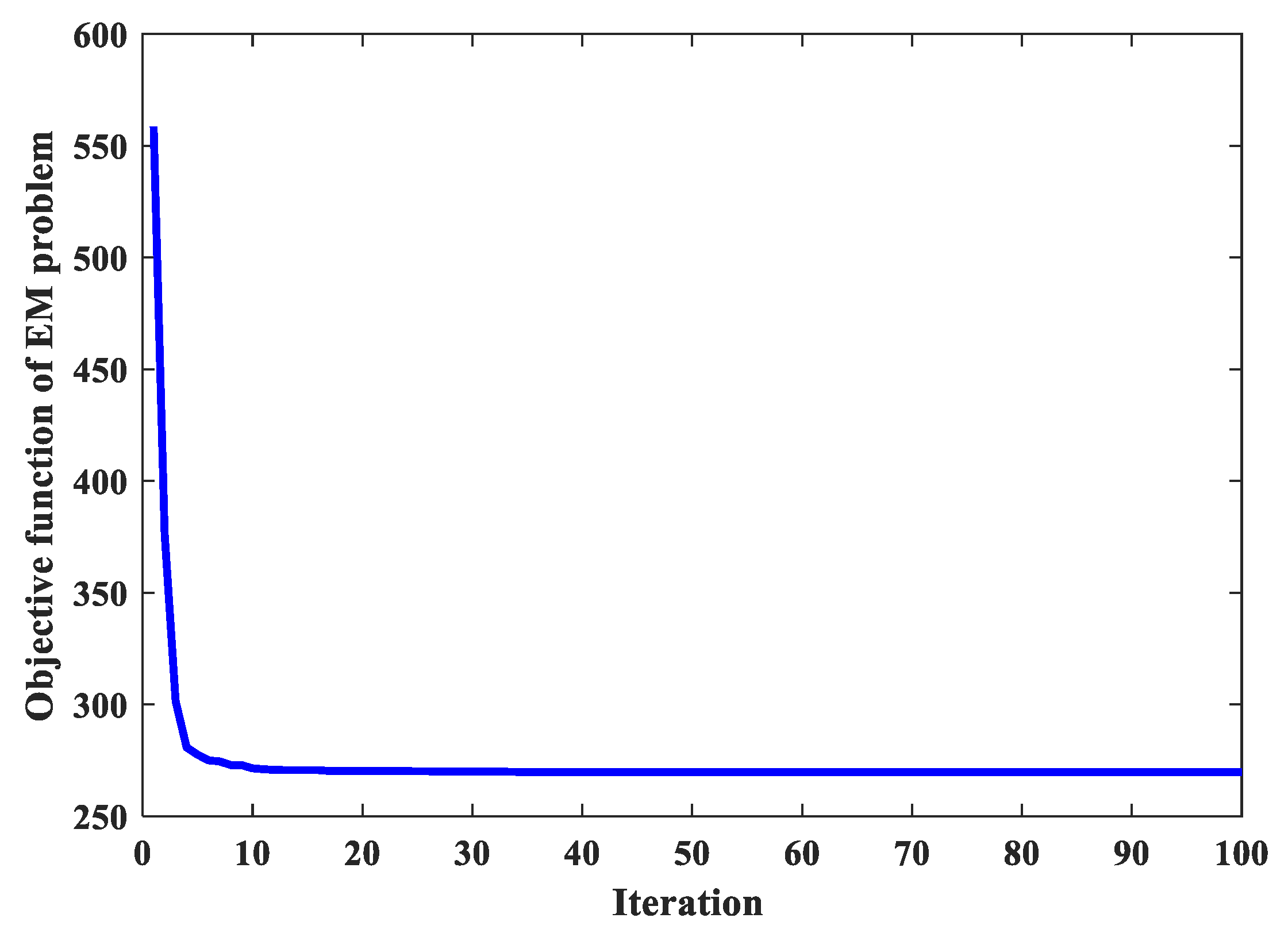
• Propose EO for solving the optimal problem of EM as an efficient technique and compare with other new techniques that are newly employed here for solving EM problem.
• Implement the proposed technique for solving the EM problem based on deterministic and probabilistic EM problems with emission.
• Investigate the effectiveness and applicability of the EO when compared with other recent optimization techniques through different scenarios.

2. The Mathematical Modeling of the EM Problem

A model of low-voltage (LV) MG connected to grid consists of different types of RESs, storage device, and loads as shown in Figure 1. The MG is connected to the utility (MV distribution network) by the MV/LV transformer. The MG central controller (MGCC) acts as an interface between the power system and the MG. The MGCC is existing downstream of utility. The functions of MGCC are designed to monitor the real and reactive power produced from DG units, maximize the MG’s value, and optimize the MG operations through sending control signal to MGs to evaluate the level of DG’s production. The local controllers (LCs) are located close to the DGs. The functions of LCs are assigned to control the MG’s components through adapting each type of DG units, controllable loads, and storage devices. Additionally, the LCs are used to control both the voltage and frequency in an islanding operating mode of MG. The optimization proceedings applied in the MGCC are based on the implemented market policy in MG operation. Most policies of operating MGs are the MGCC goal to serve the demand load of the MG through maximizing utilization of its local production. From the consumers’ point of view, the MGCC aims to minimize the total operational cost of the MG with considering DG bids, market price, and demand load through optimal adjustment of the generated power from DG units while satisfying the operational constraints [10].

2.1. The Operating Cost Function

The total operating cost of the MG system contains several DG units bids and the power exchange cost between the main grid and MG. The control variables of the optimization problem consist of the real power from the DG units including the storage units, whilst the dependent variable is the real power that is sold to or bought from the main grid. Thus, the mathematical formulation of the EM problem may be described as follows [7]:

$$\begin{gathered} {\min \mathrm{F}}_1\left(\mathrm{R}\right)={\displaystyle \sum }_{\mathrm{t}=1}^{\mathrm{T}}{\displaystyle \sum }_{\mathrm{i}=1}^{\mathrm{NG}}{\mathrm{u}}_{\mathrm{i},\mathrm{t}}{\mathrm{P}}_{\mathrm{Gi},\mathrm{t}}{\mathrm{B}}_{\mathrm{Gi},\mathrm{t}}{+\mathrm{S}}_{\mathrm{Gi},\mathrm{t}}^{\mathrm{U}}\times \max \left({0,\mathrm{u}}_{\mathrm{i},\mathrm{t}}-{\mathrm{u}}_{\mathrm{i},\mathrm{t}-1}\right){+\mathrm{S}}_{\mathrm{Gi},\mathrm{t}}^{\mathrm{D}}\times \max \left({0,\mathrm{u}}_{\mathrm{i},\mathrm{t}-1}-{\mathrm{u}}_{\mathrm{i},\mathrm{t}}\right) \\ +{\displaystyle \sum }_{\mathrm{t}=1}^{\mathrm{T}}{\displaystyle \sum }_{\mathrm{k}=1}^{\mathrm{NS}}\left[{\mathrm{u}}_{\mathrm{k},\mathrm{t}}{\mathrm{P}}_{\mathrm{Sk},\mathrm{t}}{\mathrm{B}}_{\mathrm{Sk},\mathrm{t}}{+\mathrm{S}}_{\mathrm{SK},\mathrm{t}}^{\mathrm{U}}\times \max \left({0,\mathrm{u}}_{\mathrm{k},\mathrm{t}}-{\mathrm{u}}_{\mathrm{k},\mathrm{t}-1}\right){+\mathrm{S}}_{\mathrm{SK},\mathrm{t}}^{\mathrm{D}}\times \max \left({0,\mathrm{u}}_{\mathrm{k},\mathrm{t}-1}-{\mathrm{u}}_{\mathrm{k},\mathrm{t}}\right)\right]+{\displaystyle \sum }_{\mathrm{t}=1}^{\mathrm{T}}{\mathrm{MP}}_{\mathrm{grid},\mathrm{t}}{\mathrm{P}}_{\mathrm{grid},\mathrm{t}} \end{gathered}$$

(1)

$$\mathrm{R}=\left[{\mathrm{R}}_1{,\mathrm{R}}_2{,\dots ,\mathrm{R}}_{\mathrm{t}}{,\dots ,\mathrm{R}}_{\mathrm{T}}\right]$$

(2)

where R indicates the optimal output power of different DG units, main grid, and their binary status. It is defined by:

$${\mathrm{R}}_{\mathrm{t}}=\left[{\mathrm{P}}_{\mathrm{G}1,\mathrm{t}}{,\mathrm{P}}_{\mathrm{G}2,\mathrm{t}}{,\dots ,\mathrm{P}}_{\mathrm{GNG},\mathrm{t}}{,\mathrm{P}}_{\mathrm{S}1,\mathrm{t}}{,\mathrm{P}}_{\mathrm{S}2,\mathrm{t}}{,\dots ,\mathrm{P}}_{\mathrm{SNS},\mathrm{t}}{,\mathrm{P}}_{\mathrm{grid},\mathrm{t}}{,\mathrm{u}}_{1,\mathrm{t}}{,\mathrm{u}}_{2,\mathrm{t}}{,\dots ,\mathrm{u}}_{\mathrm{NG}+\mathrm{NS},\mathrm{t}}\right]$$

(3)

From (1), it is seen that the objective function includes the total operating cost of the DG units along with their costs of startup/shutdown in the first term. The second term represents the operating cost of the ES devices with their costs of startup/shut-down. The third term is the exchange power cost between the main grid and MG.

2.2. The Pollutant Emission

The minimization of the pollutant emission includes the amount of emissions from the main grid, DG units, and ES devices in MG. There are different pollutant emissions; however, the considered important pollutants which are used to evaluate the total emission are ${\mathrm{CO}}_2, {\mathrm{SO}}_2$, and NO_x. Minimizing these emissions is considered as the second objective function that can be formulated as follows [30]:

$${\mathrm{minF}}_2\left(\mathrm{R}\right)={\displaystyle \sum }_{\mathrm{t}=1}^{\mathrm{T}}\left\{{\displaystyle \sum }_{\mathrm{i}=1}^{\mathrm{NG}}\left[{\mathrm{u}}_{\mathrm{i},\mathrm{t}}{\mathrm{P}}_{\mathrm{Gi},\mathrm{t}}{\mathrm{E}}_{\mathrm{Gi},\mathrm{t}}\right]+{\displaystyle \sum }_{\mathrm{k}=1}^{\mathrm{NS}}\left[{\mathrm{u}}_{\mathrm{k},\mathrm{t}}{\mathrm{P}}_{\mathrm{Sk},\mathrm{t}}{\mathrm{E}}_{\mathrm{Sk},\mathrm{t}}\right]{+\mathrm{E}}_{\mathrm{grid},\mathrm{t}}{\mathrm{P}}_{\mathrm{grid},\mathrm{t}}\right\}$$

(4)

Not only does the objective function include the amount of emission from the main grid, but it also considers the emissions produced from the DG units as well as the ES devices as stated in (4). The total amount of pollutants emissions are ${\mathrm{E}}_{\mathrm{grid},\mathrm{t}}$, ${\mathrm{E}}_{\mathrm{Gi},\mathrm{t}},$ and ${\mathrm{E}}_{\mathrm{Sk},\mathrm{t}}$, that can be described as follows [30]:

$${\mathrm{E}}_{\mathrm{grid},\mathrm{t}}{=\mathrm{CO}}_{2,\mathrm{t}}^{\mathrm{grid}}{+\mathrm{SO}}_{2,\mathrm{t}}^{\mathrm{grid}}+{\mathrm{NO}}_{\mathrm{x},\mathrm{t}}^{\mathrm{grid}}$$

(5)

$${\mathrm{E}}_{\mathrm{Gi},\mathrm{t}}{=\mathrm{CO}}_{2,\mathrm{t}}^{\mathrm{Gi}}+{\mathrm{SO}}_{2,\mathrm{t}}^{\mathrm{Gi}}+{\mathrm{NO}}_{\mathrm{x},\mathrm{t}}^{\mathrm{Gi}}$$

(6)

$${\mathrm{E}}_{\mathrm{Sk},\mathrm{t}}{=\mathrm{CO}}_{2,\mathrm{t}}^{\mathrm{Sk}}+{\mathrm{SO}}_{2,\mathrm{t}}^{\mathrm{Sk}}+{\mathrm{NO}}_{\mathrm{x},\mathrm{t}}^{\mathrm{Sk}}+$$

(7)

2.3. Constraints of Power Sources

2.3.1. The Constraint of Power Balance

The total generated power from DG units, ES devices, and the main grid must supply the total load demand of the MG at each period t. However, the active power losses are neglected in the MG. Accordingly, the constraints of the power balance equation can be expressed as follows [31]:

$${\mathrm{P}}_{\mathrm{grid},\mathrm{t}}+{\displaystyle \sum }_{\mathrm{i}=1}^{\mathrm{NG}}{\mathrm{P}}_{\mathrm{Gi},\mathrm{t}}+{\displaystyle \sum }_{\mathrm{k}=1}^{\mathrm{NS}}{\mathrm{P}}_{\mathrm{Sk},\mathrm{t}}-{\displaystyle \sum }_{\mathrm{j}=1}^{\mathrm{ND}}{\mathrm{P}}_{\mathrm{Dj},\mathrm{t}}=0$$

(8)

2.3.2. Constraints of Power Generation

The energy generated from each DG unit, ES devices, and the main grid should be limited in the range of its defined capacity.

$${\mathrm{P}}_{\mathrm{Gi},\mathrm{t}}^{\min }\le {\mathrm{P}}_{\mathrm{Gi},\mathrm{t}}\le {\mathrm{P}}_{\mathrm{Gi},\mathrm{t}}^{\max }$$

(9)

$${\mathrm{P}}_{\mathrm{Sk},\mathrm{t}}^{\min }\le {\mathrm{P}}_{\mathrm{Sk},\mathrm{t}}\le {\mathrm{P}}_{\mathrm{Sk},\mathrm{t}}^{\max }$$

(10)

$${\mathrm{P}}_{\mathrm{grid},\mathrm{t}}^{\min }\le {\mathrm{P}}_{\mathrm{grid},\mathrm{t}}\le {\mathrm{P}}_{\mathrm{grid},\mathrm{t}}^{\max }$$

(11)

2.3.3. Spinning Reserve

It is necessary to maintain the power system reliability due to the continuous fluctuations in RESs. However, for achieving the spinning reserve, the following expression should be employed [10].

$${\mathrm{P}}_{\mathrm{grid},\mathrm{t}}^{\max }+{\displaystyle \sum }_{\mathrm{i}=1}^{\mathrm{NG}}{\mathrm{u}}_{\mathrm{i},\mathrm{t}}{\mathrm{P}}_{\mathrm{Gi},\mathrm{t}}^{\max }+{\displaystyle \sum }_{\mathrm{k}=1}^{\mathrm{NS}}{\mathrm{u}}_{\mathrm{k},\mathrm{t}}{\mathrm{P}}_{\mathrm{Sk},\mathrm{t}}^{\max }\ge {\displaystyle \sum }_{\mathrm{j}=1}^{\mathrm{ND}}{\mathrm{P}}_{\mathrm{Dj},\mathrm{t}}+{\mathrm{R}}_{\mathrm{e},\mathrm{t}}$$

(12)

2.3.4. Constraints of Energy Storage Devices

Concerning ES devices, the amount of stored energy and the limits on the charge and discharge rate of these ES devices during each time t interval with the constraints are defined as [10]:

$${\mathrm{E}}_{\mathrm{es},\mathrm{t}}{=\mathrm{E}}_{\mathrm{es},\mathrm{t}-1}{+\mathsf{\eta }}_{\mathrm{chr}}{\mathrm{P}}_{\mathrm{chr}}\mathsf{\Delta }\mathrm{t}-\left({1/\mathsf{\eta }}_{\mathrm{dischr}}\right){\mathrm{P}}_{\mathrm{dischr}} \mathsf{\Delta }\mathrm{t}$$

(13)

$${\mathrm{E}}_{\mathrm{es}}^{\min }\le {\mathrm{E}}_{\mathrm{es},\mathrm{t}}\le {\mathrm{E}}_{\mathrm{es}}^{\max }$$

(14)

$${\mathrm{P}}_{\mathrm{chr},\mathrm{t}}\le {\mathrm{P}}_{\mathrm{chr}}^{\max }$$

(15)

$${\mathrm{P}}_{\mathrm{dischr},\mathrm{t}}\le {\mathrm{P}}_{\mathrm{dischr}}^{\max }$$

(16)

2.4. The Optimization Problem

The total demand load is supplied from the sources of MG by the local production, as available. Therefore, the output power from the main grid ${\mathrm{P}}_{\mathrm{grid},\mathrm{t}}$ is set as a dependent variable for enforcing the power balance equation constraint. However, the power from the main grid is determined from (8) as follows:

$${\mathrm{P}}_{\mathrm{grid},\mathrm{t}}={\displaystyle \sum }_{\mathrm{j}=1}^{\mathrm{ND}}{\mathrm{P}}_{\mathrm{Dj},\mathrm{t}}-{\displaystyle \sum }_{\mathrm{i}=1}^{\mathrm{NG}}{\mathrm{P}}_{\mathrm{Gi},\mathrm{t}}-{\displaystyle \sum }_{\mathrm{k}=1}^{\mathrm{NS}}{\mathrm{P}}_{\mathrm{Sk},\mathrm{t}}$$

(17)

The constraints can be handled by converting it into unconstrained one using the penalty function technique. However, the penalty factors with the constraints are involved into the objective function as quadratic penalty terms. Further, the goal of the penalty factors that are chosen as positive large values is to reduce the impractical solutions [32]. Therefore, ${\mathrm{P}}_{\mathrm{grid},\mathrm{t}}$ is added as a quadratic penalty term to the objective function in (1). Consequently, the new extended objective function by the penalty factor becomes:

$$\begin{gathered} {\mathrm{minF}}_1\left(\mathrm{R}\right)={\displaystyle \sum }_{\mathrm{t}=1}^{\mathrm{T}}{\displaystyle \sum }_{\mathrm{i}=1}^{\mathrm{NG}}\left[{\mathrm{u}}_{\mathrm{i},\mathrm{t}}{\mathrm{P}}_{\mathrm{Gi},\mathrm{t}}{\mathrm{B}}_{\mathrm{Gi},\mathrm{t}}{+\mathrm{S}}_{\mathrm{Gi},\mathrm{t}}^{\mathrm{U}}\text{×}\max \left({0,\mathrm{u}}_{\mathrm{i},\mathrm{t}}-{\mathrm{u}}_{\mathrm{i},\mathrm{t}-1}\right){+\mathrm{S}}_{\mathrm{Gi},\mathrm{t}}^{\mathrm{D}}\text{×}\max \left({0,\mathrm{u}}_{\mathrm{i},\mathrm{t}-1}-{\mathrm{u}}_{\mathrm{i},\mathrm{t}}\right)\right] \\ +{\displaystyle \sum }_{\mathrm{t}=1}^{\mathrm{T}}{\displaystyle \sum }_{\mathrm{k}=1}^{\mathrm{NS}}\left[{\mathrm{u}}_{\mathrm{k},\mathrm{t}}{\mathrm{P}}_{\mathrm{Sk},\mathrm{t}}{\mathrm{B}}_{\mathrm{Sk},\mathrm{t}}{+\mathrm{S}}_{\mathrm{SK},\mathrm{t}}^{\mathrm{U}}\text{×}\max \left({0,\mathrm{u}}_{\mathrm{k},\mathrm{t}}-{\mathrm{u}}_{\mathrm{k},\mathrm{t}-1}\right){+\mathrm{S}}_{\mathrm{SK},\mathrm{t}}^{\mathrm{D}}\text{×}\max \left({0,\mathrm{u}}_{\mathrm{k},\mathrm{t}-1}-{\mathrm{u}}_{\mathrm{k},\mathrm{t}}\right)\right] \\ +{\displaystyle \sum }_{\mathrm{t}=1}^{\mathrm{T}}{\mathrm{MP}}_{\mathrm{grid},\mathrm{t}}{\mathrm{P}}_{\mathrm{grid},\mathrm{t}}+\mathsf{\gamma }{\left({\mathrm{P}}_{\mathrm{grid},\mathrm{t}}-{\mathrm{P}}_{\mathrm{grid},\mathrm{t}}^{\lim }\right)}^2 \end{gathered}$$

(18)

In this paper, the above two objective functions: the minimization of both cost and pollution emission of MGs, are integrated. The multi-objective function is converted into a single objective function using the coefficients and price penalty terms. Moreover, the price penalty function for each generating unit is defined as the ratio between the operating cost and the pollution emission. There are various types of price penalty techniques as discussed in [33]. Here, the max/max price penalty factor is utilized. Consequently, the developed objective function can be described as follows:

$$\begin{gathered} {\mathrm{minF}}_{\mathrm{t}}\left(\mathrm{R}\right)={\displaystyle \sum }_{\mathrm{t}=1}^{\mathrm{T}}{\displaystyle \sum }_{\mathrm{i}=1}^{\mathrm{NG}}\left[{\mathrm{u}}_{\mathrm{i},\mathrm{t}}{\mathrm{P}}_{\mathrm{Gi},\mathrm{t}}{\mathrm{B}}_{\mathrm{Gi},\mathrm{t}}{+\mathrm{S}}_{\mathrm{Gi},\mathrm{t}}^{\mathrm{U}}\text{×}\max \left({0,\mathrm{u}}_{\mathrm{i},\mathrm{t}}-{\mathrm{u}}_{\mathrm{i},\mathrm{t}-1}\right)+{\mathrm{S}}_{\mathrm{Gi},\mathrm{t}}^{\mathrm{D}}\text{×}\max \left({0,\mathrm{u}}_{\mathrm{i},\mathrm{t}-1}-{\mathrm{u}}_{\mathrm{i},\mathrm{t}}\right)\right] \\ +{\displaystyle \sum }_{\mathrm{t}=1}^{\mathrm{T}}{\displaystyle \sum }_{\mathrm{k}=1}^{\mathrm{NS}}\left[{\mathrm{u}}_{\mathrm{k},\mathrm{t}}{\mathrm{P}}_{\mathrm{Sk},\mathrm{t}}{\mathrm{B}}_{\mathrm{Sk},\mathrm{t}}{+\mathrm{S}}_{\mathrm{SK},\mathrm{t}}^{\mathrm{U}}\text{×}\max \left({0,\mathrm{u}}_{\mathrm{k},\mathrm{t}}-{\mathrm{u}}_{\mathrm{k},\mathrm{t}-1}\right){+\mathrm{S}}_{\mathrm{SK},\mathrm{t}}^{\mathrm{D}}\text{×}\max \left({0,\mathrm{u}}_{\mathrm{k},\mathrm{t}-1}-{\mathrm{u}}_{\mathrm{k},\mathrm{t}}\right)\right]+{\displaystyle \sum }_{\mathrm{t}=1}^{\mathrm{T}}{\mathrm{MP}}_{\mathrm{grid},\mathrm{t}}{\mathrm{P}}_{\mathrm{grid},\mathrm{t}} \\ +{\displaystyle \sum }_{\mathrm{t}=1}^{\mathrm{T}}\mathsf{\Psi }\left[{\displaystyle \sum }_{\mathrm{i}=1}^{\mathrm{NG}}{\mathrm{u}}_{\mathrm{i},\mathrm{t}}{\mathrm{P}}_{\mathrm{Gi},\mathrm{t}}{\mathrm{E}}_{\mathrm{Gi},\mathrm{t}}+{\displaystyle \sum }_{\mathrm{k}=1}^{\mathrm{NS}}{\mathrm{u}}_{\mathrm{k},\mathrm{t}}{\mathrm{P}}_{\mathrm{Sk},\mathrm{t}}{\mathrm{E}}_{\mathrm{Sk},\mathrm{t}}{+\mathrm{E}}_{\mathrm{grid},\mathrm{t}}{\mathrm{P}}_{\mathrm{grid},\mathrm{t}}\right]+\mathsf{\gamma }{\left({\mathrm{P}}_{\mathrm{grid},\mathrm{t}}-{\mathrm{P}}_{\mathrm{grid},\mathrm{t}}^{\lim }\right)}^2 \end{gathered}$$

(19)

3. Probabilistic EM of the MG

The probabilistic formulation problem requires representation of the input random variables, statistically. Solving the EM problem based on the probabilistic approach has two key steps. In the first step, the input random variables are characterized statistically. The source of the uncertainty for the dependent variables in the system arise from the uncertainty of the independent input random variables. Furthermore, due to the random nature of input variables such as the variations of demand load, output power from DG units, and market prices, the obtained EM results such as the total operating cost of the system should be considered as a random variable. Evaluation of the statistical characteristics for the EM result is the second step in the probabilistic EM approach. However, in the case of one or more uncertain input variables, the EM problem turns into a probabilistic problem.

3.1. The Statistical Characterization of Input Random Variables

Evaluating the output power of WT mainly depends on two factors: the power curve of WT and the wind speed at a specific location, as described in [34] as follows:

$${\mathrm{P}}_{\mathrm{WT}}=\{\begin{array}{c}0\mathsf{\nu }\le {\mathsf{\nu }}_{\mathrm{ci}}{\hspace{1em}\mathsf{\nu }>\mathsf{\nu }}_{\mathrm{co}}\\ \frac{{\mathsf{\nu }}^2-{\mathsf{\nu }}_{\mathrm{ci}}^2}{{\mathsf{\nu }}_{\mathrm{nom}}^2-{\mathsf{\nu }}_{\mathrm{ci}}^2}{·\mathrm{P}}_{\mathrm{nom}}\hspace{1em}{\mathsf{\nu }}_{\mathrm{ci}}<\mathsf{\nu }\le {\mathsf{\nu }}_{\mathrm{nom}}\\ {\mathrm{P}}_{\mathrm{nom}}{\mathsf{\nu }}_{\mathrm{nom}}<\mathsf{\nu }\le {\mathsf{\nu }}_{\mathrm{co}}\end{array}$$

(20)

Likewise, the output power of the PV depends on both the solar irradiance and the ambient air temperature of the PV. The output power of PV can be computed as described in [35] as follows:

$${\mathrm{P}}_{\mathrm{PV}}=\frac{{\mathrm{P}}_{\mathrm{STC}}{\mathrm{I}}_{\mathrm{S}}}{1000}{[1+\mathsf{\beta }(\mathrm{T}}_{\mathrm{C}}-25\left)\right]$$

(21)

where, the temperature of PV module can be determined as follows:

$${\mathrm{T}}_{\mathrm{C}}{=\mathrm{T}}_{\mathrm{A}}+\frac{{\mathrm{I}}_{\mathrm{S}}}{800}{(\mathrm{T}}_{\mathrm{NOCT}}-20)$$

(22)

3.1.1. Modeling of Wind Speed

At a specific location, the probability density function (PDF) of the wind speed, as well as the output power of WT, can be described by a Weibull distribution as in [34] as follows:

$${\mathrm{f}}_{\mathsf{\nu }}\left(\mathsf{\nu }\right)=\frac{\mathrm{K}}{\mathrm{C}}·(\frac{\mathsf{\nu }}{\mathrm{C}}{)}^{\mathrm{K}-1}{·\mathrm{e}}^{-{(\raisebox{1ex}{$\mathsf{\nu }$}\!\left/ \!\raisebox{-1ex}{$\mathrm{C}$}\right.)}^{\mathrm{K}}}$$

(23)

For the Weibull distribution, the cumulative density function (CDF) is:

$${\mathrm{F}}_{\mathsf{\nu }}\left(\mathsf{\nu }\right)=1-{\mathrm{e}}^{-{(\raisebox{1ex}{$\mathsf{\nu }$}\!\left/ \!\raisebox{-1ex}{$\mathrm{C}$}\right.)}^{\mathrm{K}}}$$

(24)

For calculating the wind speed, the CDF as well as its inverse has been used as follows:

$$\mathsf{\nu }=\mathrm{C}·(-{\ln \left(\mathrm{r}\right))}^{\raisebox{1ex}{$1$}\!\left/ \!\raisebox{-1ex}{$\mathrm{K}$}\right.}$$

(25)

The parameters of the Weibull distribution can be calculated as follows:

$$\mathrm{K}=(\frac{\mathsf{\sigma }}{{\mathsf{\nu }}_{\mathrm{m}}}{)}^{-1.086}$$

(26)

$$\mathrm{C}=\frac{{\mathsf{\nu }}_{\mathrm{m}}}{\Gamma (1+\raisebox{1ex}{$1$}\!\left/ \!\raisebox{-1ex}{$\mathrm{K}$}\right.)}$$

(27)

where the gamma function $\Gamma \mathrm{x}$ is described as:

$$\Gamma \mathrm{x}={{\displaystyle \int }}_0^{\infty }{\mathrm{t}}^{\mathrm{x}-1}{\mathrm{e}}^{-\mathrm{t}} \mathrm{dt},\hspace{1em}\mathrm{x}>0$$

(28)

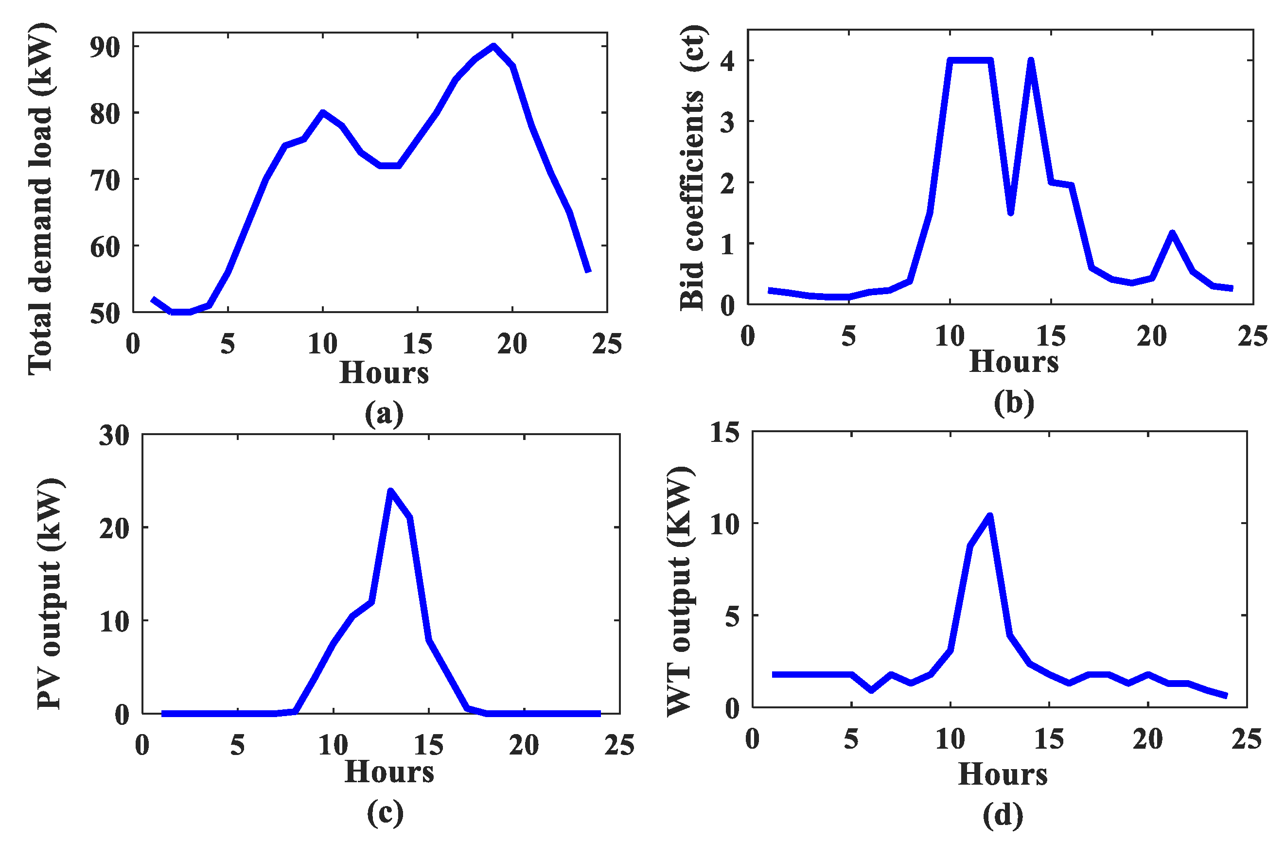
3.1.2. Modeling of Solar Irradiance, Market-Price, and Load Demand

In this paper, it was suggested that the solar irradiance, market price, and demand of load have a normal distribution function. Therefore, the corresponding PDF of any variable ${\mathrm{z}}_{\mathrm{i}}$ can be formulated as follows [10,35]:

$${\mathrm{f}}_{{\mathrm{z}}_{\mathrm{i}}}{(\mathrm{z}}_{\mathrm{i}})=\frac{1}{\mathsf{\sigma }\sqrt{2\mathsf{\pi }}}·{\mathrm{e}}^{-\left(\raisebox{1ex}{${{(\mathrm{z}}_{\mathrm{i}}-\mathsf{\mu })}^2$}\!\left/ \!\raisebox{-1ex}{${\mathsf{\sigma }}^2$}\right.\right)}$$

(29)

Additionally, the CDF for the normal distribution can be computed by:

$${\mathrm{F}}_{{\mathrm{z}}_{\mathrm{i}}}\left({\mathrm{z}}_{\mathrm{i}}\right)=\frac{1}{2}\left[1+\mathrm{erf}\left(\frac{{\mathrm{z}}_{\mathrm{i}}-\mathsf{\mu }}{\mathsf{\sigma }\sqrt{2}}\right)\right]$$

(30)

For determining the variable ${\mathrm{z}}_{\mathrm{i}},$ the CDF and its inverse has been used as follows:

$${\mathrm{z}}_{\mathrm{i}}=\mathsf{\mu }+\sqrt{2}·\sigma ·{\mathrm{erf}}^1(2\mathrm{r}-1)$$

(31)

where, the error function and its inverse are defined as follows:

$$\mathrm{erf}\left(\mathrm{z}\right)=\frac{2}{\sqrt{\pi }}{{\displaystyle \int }}_0^z{\mathrm{e}}^{-{\mathrm{t}}^2}\mathrm{dt}$$

(32)

$${\mathrm{erf}}^{-1}\left(\mathrm{Z}\right)=1-\mathrm{erf}\left(\mathrm{z}\right)$$

(33)

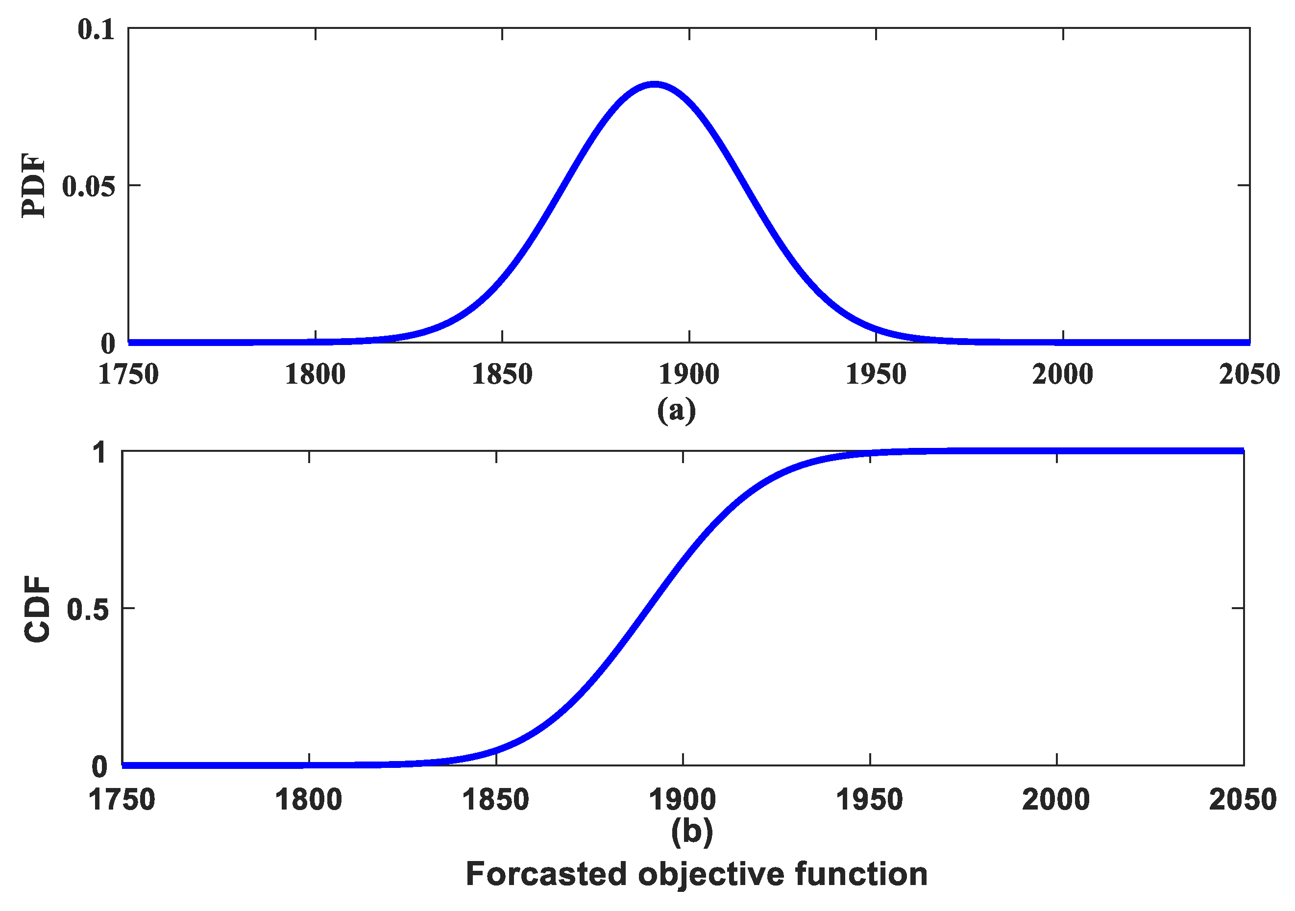
3.2. Statistical Evaluation of the Output

In order to formulate the probabilistic problem, it is necessary to characterize the input random variables in a statistical nature as well as the method for evaluating the output variables statistically. The probabilistic EM can be formulated mathematically as follows:

$$\mathrm{V}=\mathrm{f}\left(\mathrm{I}\right)$$

(34)

There are several statistical approaches for handling the output variables as introduced in some literature, in which they are classified into three categories: analytical methods, approximation approaches, and the Monte Carlo simulation (MCS). The MCS randomly generates many uncertain input variables, then uses these values to solve a deterministic problem. The simulation process is repeated many times (hundreds to thousands) to attain an acceptable accuracy for the statistical characteristics of the output results. The major problem of using MCS is the large number of simulations that are required to achieve convergence.

The point estimation approach is considered one of the approximation approaches that present a convergent description of the statistical output random variables. This method, like MCS, employs a deterministic approach for solving a probabilistic problem but over a much lower number of the simulations that is implemented in MCS. Moreover, this method guarantees a considerable reduction in the calculation’s efforts compared to the MCS.

The basic idea of the point estimation approach is to focus on the information collected from few forecasted values of the m input variables on K = 2 points for each interest input variable that are called central moments. Using these two central moments for each input, the output variables are calculated in the form of statistical moments 2m + 1 times for selected uncertain input variables [10]. Depending on the statistical moments, the PDF of output random variables of interest can be approximated based on the Gram–Charlier series approach [36].

The following steps of the 2m + 1 point estimation method can be summarized as follows:

Step 1: Define the number of selected uncertain inputs.

Step 2: Set the output variable vector of the jth moment $\mathrm{E}\left({\mathrm{V}}^{\mathrm{j}}\right)=0$.

Step 3: Set $\mathrm{r}=1 (\mathrm{r}=1, 2, \dots , \mathrm{m}).$

Step 4: Set the uncertain parameter ${\mathrm{z}}_{\mathrm{r}}$.

Step 5: Calculate the two standard locations of the variable ${\mathrm{z}}_{\mathrm{r}}$:

$${\mathsf{\zeta }}_{\mathrm{r},\mathrm{l}}=\frac{{\mathsf{\lambda }}_{\mathrm{r},3}}{2}+{\left(-1\right)}^{3-\mathrm{l}}\times \sqrt{{\mathsf{\lambda }}_{\mathrm{r},4}-\frac{{3\mathsf{\lambda }}_{\mathrm{r},3}^2}{4}}\mathrm{l}=1, 2$$

(35)

Step 6: Define the two locations of ${\mathrm{z}}_{\mathrm{r}}$:

$${\mathrm{z}}_{\mathrm{r},\mathrm{l}}{=\mathsf{\mu }}_{{\mathrm{z}}_{\mathrm{r}}}{+\mathsf{\zeta }}_{\mathrm{r},\mathrm{l}}{\times \mathsf{\sigma }}_{{\mathrm{z}}_{\mathrm{r}}}\mathrm{l}=1, 2$$

(36)

Step 7: Run the deterministic EM based on the optimization algorithm for both locations ${\mathrm{z}}_{\mathrm{r}}$.

$${\mathrm{V}}_{\mathrm{r},\mathrm{l}}=\mathrm{f}\left({\mathsf{\mu }}_{{\mathrm{z}}_1}{,\mathsf{\mu }}_{{\mathrm{z}}_2}{,\dots ,\mathrm{z}}_{\mathrm{r},\mathrm{l}}{,\dots ,\mathsf{\mu }}_{{\mathrm{z}}_{\mathrm{m}}}\right)\mathrm{l}=1, 2$$

(37)

Step 8: Determine two weight factors of ${\mathrm{z}}_{\mathrm{r}}:$

$${\mathrm{w}}_{\mathrm{r},\mathrm{l}}=\frac{{\left(-1\right)}^{3-\mathrm{l}}}{{\mathsf{\zeta }}_{\mathrm{r},\mathrm{l}}\left({\mathsf{\zeta }}_{\mathrm{r},1}-{\mathsf{\zeta }}_{\mathrm{r},2}\right)}=1, 2$$

(38)

Step 9: Update ${\mathrm{E}(\mathrm{V}}^{\mathrm{k}}$).

$$\mathrm{E}\left({\mathrm{V}}^{\mathrm{j}}\right)=\mathrm{E}\left({\mathrm{V}}^{\mathrm{j}}\right)+{\displaystyle \sum }_{\mathrm{l}=1}^2{\mathrm{w}}_{\mathrm{r},\mathrm{l}}{\left({\mathrm{V}}_{\mathrm{r},\mathrm{l}}\right)}^{\mathrm{j}}$$

(39)

Step 10: Repeat Steps 5–9 for $\mathrm{r}=\mathrm{r}+1$ until the selected random inputs are taken.

Step 11: Compute the deterministic EM based on the following vector:

$${\mathrm{z}}_{\mathsf{\mu }}=\left[{\mathsf{\mu }}_{{\mathrm{z}}_1}{,\mathsf{\mu }}_{{\mathrm{z}}_2}{,\dots ,\mathsf{\mu }}_{\mathrm{z},\mathrm{r}}{,\dots ,\mathsf{\mu }}_{{\mathrm{z}}_{\mathrm{m}}}\right]\mathrm{l}=1, 2$$

(40)

Step 12: Determine the weight factor for the EM problem obtained in step 11:

$${\mathrm{w}}_0=1-{\displaystyle \sum }_{\mathrm{r}=1}^{\mathrm{m}}\frac{1}{{\mathsf{\lambda }}_{\mathrm{r},4}{-\mathsf{\lambda }}_{\mathrm{r},3}^2}$$

(41)

Step 13: Update ${\mathrm{E}(\mathrm{V}}^{\mathrm{j}}$)

$$\mathrm{E}\left({\mathrm{V}}^{\mathrm{j}}\right)={\displaystyle \sum }_{\mathrm{r}=1}^{\mathrm{m}}{\displaystyle \sum }_{\mathrm{l}=1}^2{\mathrm{w}}_{\mathrm{r},\mathrm{l}}{\left[\left({\mathsf{\mu }}_{{\mathrm{z}}_1}{,\mathsf{\mu }}_{{\mathrm{z}}_2}{,\dots ,\mathrm{z}}_{\mathrm{r},\mathrm{l}}{,\dots ,\mathsf{\mu }}_{{\mathrm{z}}_{\mathrm{m}}}\right)\right]}^{\mathrm{j}}{+\mathrm{w}}_0{\left[\mathrm{V}\left({\mathrm{z}}_{\mathsf{\mu }}\right)\right]}^{\mathrm{j}}$$

(42)

Step 14: After obtaining the output statistical moments, the $\mathsf{\mu }$ and $\mathsf{\sigma }$ can be computed:

$${\mathsf{\mu }}_{\mathrm{V}}=\mathrm{E}\left(\mathrm{V}\right){; \mathsf{\sigma }}_{\mathrm{V}}=\sqrt{\mathrm{E}\left({\mathrm{V}}^2\right)-{\mathsf{\mu }}_{\mathrm{V}}^2}$$

(43)

Depending on the values of $\mathsf{\mu }$ and $\mathsf{\sigma }$ along with the method of Gram–Charlier as in [36], PDF and CDF are calculated for the output random variable.

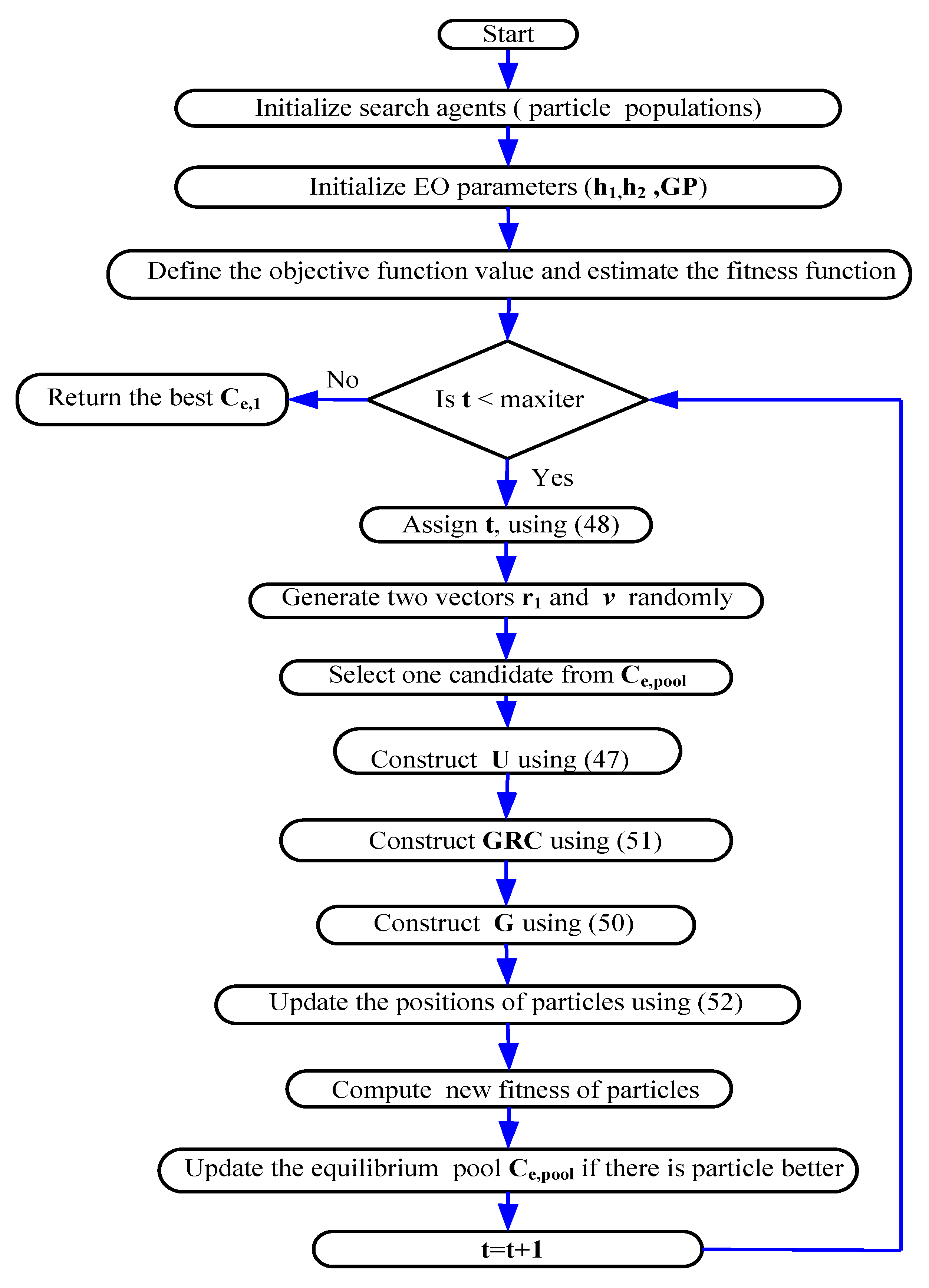
4. The Equilibrium Optimizer Algorithm Overview

The EO algorithm is inspired by the analytical solution of a well-mixed dynamic equilibrium in a control volume. The balance equation of mass is utilized to describe the nonreactive constituent concentration on a control volume. It is known that the balance equation plays an important role in providing principles of physics to maintain the mass produced entering and leaving a control volume. Like other several recent optimization algorithms, at the beginning of the optimization procedure of EO, a random population is generated in the dimensional of search space for the optimization problem, where the particle acts as a solution and the concentration acts as the position of the particle [28].

According to the number of particles, the population and the dimensions of search space and the uniform random initialization of the initial concentrations are described as follows:

$${\mathrm{C}}_{\mathrm{d}}^{\mathrm{k}}{=\mathrm{C}}_{\mathrm{d}}^{\min }+\left({\mathrm{C}}_{\mathrm{d}}^{\max }-{\mathrm{C}}_{\mathrm{d}}^{\min }\right){\times \mathrm{rand}}_{\mathrm{d}}^{\mathrm{k}}\mathrm{k}=1,2,\dots ,\mathrm{m}$$

(44)

At the beginning of the search process, the concentration degree along with the equilibrium state is unknown. For providing a search style of particles, only the equilibrium candidate is calculated. However, for estimating the equilibrium candidate solutions, the fitness function of all particles is evaluated, then the best scores are saved and sorted. The end convergence state is called the equilibrium state which is called the global optimal solution.

Based on various experiments of optimization problems, the EO algorithm allocates the four best particle solutions in the generated population at equilibrium candidate solutions during the implementation of the whole optimization procedure in addition to another particle having a concentration equal to the mean value of the previous proper four best solutions. However, these five candidate solutions are stored in a vector, which is called an equilibrium pool.

It worth noting that the four particle candidates make the EO algorithm capable of improving the exploration, while others support the exploitation process [27].

$${\mathrm{C}}_{\mathrm{e},\mathrm{pool}}{=\text{{}\mathrm{C}}_{\mathrm{e},1}{,\mathrm{C}}_{\mathrm{e},2}{,\mathrm{C}}_{\mathrm{e},3}{,\mathrm{C}}_{\mathrm{e},4}{,\mathrm{C}}_{\mathrm{e},\mathrm{mean}}\text{}}$$

(45)

For each iteration, the particle concentration is updated using a random style between the selected candidates that are selected with the same probability. However, in the first iteration, the first selected particle will update all concentrations based on C. Then, in the second iteration, the concentrations of the same selected particle are updated based on ${\mathrm{C}}_{\mathrm{e},\mathrm{mean}}$. The updating process is repeated for each particle until reaching the process end. The exponential parameter term $\mathrm{U}$ contributes to the concentration updating rule for achieving the appropriate balance between exploitation and exploration, where it is computed as follows:

$$\mathrm{U}=\exp (-\mathsf{\nu }\left(\mathrm{t}-{\mathrm{t}}_0\right))$$

(46)

The value of t is reduced while the iteration number increased.

$$\mathrm{t}={\left(1-\mathrm{itr}/\mathrm{maxitr}\right)}^{\left({\mathrm{h}}_2\times \mathrm{itr}/\mathrm{maxitr}\right)}$$

(47)

$${\mathrm{t}}_0=\mathrm{t}+1/\mathsf{\nu }\times \ln \left({-\mathrm{h}}_1\mathrm{sign}\left({\mathrm{r}}_1-0.5\right)\left[1-\exp (-\mathsf{\nu }\mathrm{t})\right]\right)$$

(48)

However, the component $\mathrm{sign}\left({\mathrm{r}}_1-0.5\right)$ has an impact on the directions of both exploration and exploitation. The following formula should be implemented for improving the capability of both the exploration and exploitation of the EO algorithm to guarantee convergence. To improve the exploitation phase, the generation rate is developed as the most important step in the procedure of the EO algorithm for providing the optimal solution.

$$\mathrm{G}=\mathrm{GRC}\times \left({\mathrm{C}}_{\mathrm{e}}-\mathsf{\nu }\mathrm{C}\right)\times \exp (-\mathsf{\delta }\left(\mathrm{t}-{\mathrm{t}}_0\right))$$

(49)

$$\mathrm{GRC}=\{\begin{array}{c}0.5{\mathrm{r}}_2{\mathrm{if}\mathrm{r}}_3\ge \mathrm{GP}\\ {0\mathrm{if}\mathrm{r}}_3\le \mathrm{GP}\end{array}$$

(50)

where the updating rule of the EO algorithm is as follows:

$${\mathrm{C}=\mathrm{C}}_{\mathrm{e}}+\left(\mathrm{C}-{\mathrm{C}}_{\mathrm{e}}\right)\mathrm{U}+\mathrm{G}\times 1/\mathsf{\nu }\times \left(1-\mathrm{U}\right)$$

(51)

The second term will be set to find an optimal position through globally searching the space upon its discovering a position. The third term will contribute to making the solution more accurate. The added memory is utilized to store the procedures and assist the individual particle to follow the path of its coordinates in the dimension of search space and notify it about its better score. The fittest value of every particle in the current iteration is compared to an identical value in the previous iteration and will be stored if it results in an improved value. This procedure assists the ability of exploitation but may raise the chance of falling in local minima if the technique does not achieve benefit from the ability of global exploration. More details of the EO algorithm are reported in [27]. Figure 2 shows the flowchart of the EO.

5. The Simulation Results

To prove the effectiveness of the EO algorithm for solving both deterministic and probabilistic EM problems with the consideration of the emission from RESs as well as ES devices in the MG system, the EO is investigated through the MG test system shown in Figure 1. The system is considered in the grid-connected mode at a low-voltage level. The MG consists of different technologies of DG sources. These sources are the PV, WT, microturbine (MT), proton-exchange membrane fuel cell (PEM-FC), and a storage device such as a NiMH-battery [30,31]. The MG is connected to the main grid via a power transformer.

The power is exchanged between the main grid and MG according to the decisions from the control center of MG for trading energy. Further, all MG sources only produce active power at unity power factor. Moreover, the demand loads inside MG during the day consist of one feeder for supplying light commercial loads, a second feeder for serving the residential region, and the third feeder for supplying a small industrial load. However, approximately the total demand load is equivalent to 1695 kWh per day. The study is carried out for the next day (24 h) at different loads. The data of the MG system are detailed and taken from [7,10,24].

Table 1. The power limitations, bid coefficients, and emissions of the MG sources.

ID	Type	Min. Power (kW)	Max. Power (kW)	BGi (EUR/kW h)	CO2 (kg/MWh)	SO2 (kg/MWh)	NOx (kg/MWh)
1	MT	6	30	0.457	720	0.0036	0.1
2	FC	3	30	0.294	460	0.003	0.0075
3	PV	0	25	2.584	0	0	0
4	WT	0	15	1.073	0	0	0
5	Battery	−30	30	0.38	10	0.0002	0.001
6	Utility	−30	30	-	922	3.583	2.295

displays the minimum and maximum generation, the bid coefficients, and the emissions of MGs [8,30]. The forecasted demand load bid coefficients of the main grid and the expected output power of PV and WT over one day are shown in Figure 3 [10].

In this study, the important parameters of the EO algorithm are chosen before its applications for solving the EM optimization problem. These parameters are computed using experimental tests. In addition, all simulation evaluations have been executed using MATLAB 2016b on a 2.9-GHz i7 PC with 16-GB of RAM. The EO is applied to compute EM in both deterministic and probabilistic manners according to three considered scenarios:

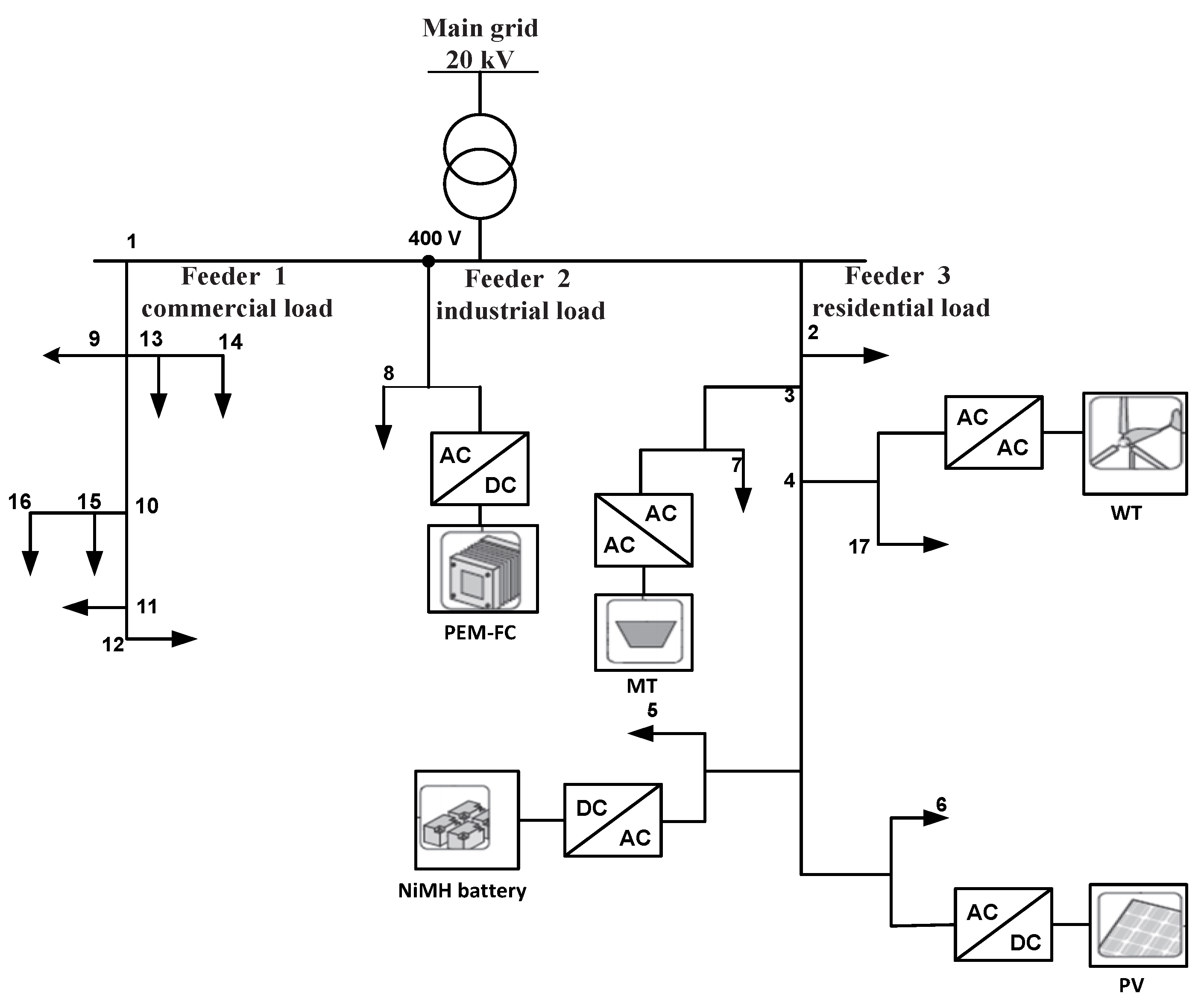
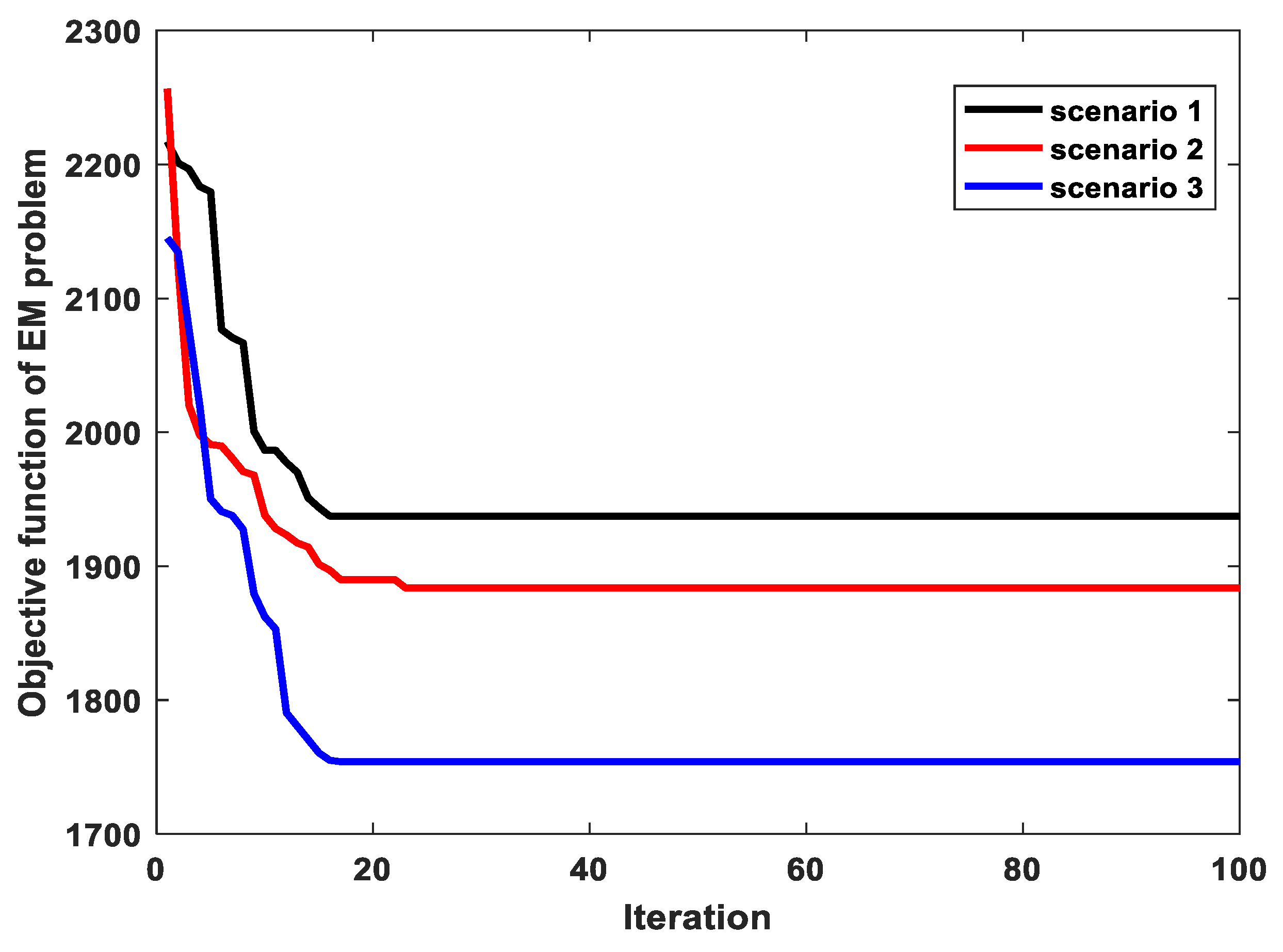
• Scenario 1: It is supposed that all MG sources operate over the examined interval. The PV and WT are represented to deliver the forecasted maximum output power during each hour. In contrast, the main grid, PEMFC, MT, and battery operate according to their output power limits for achieving the constraints.
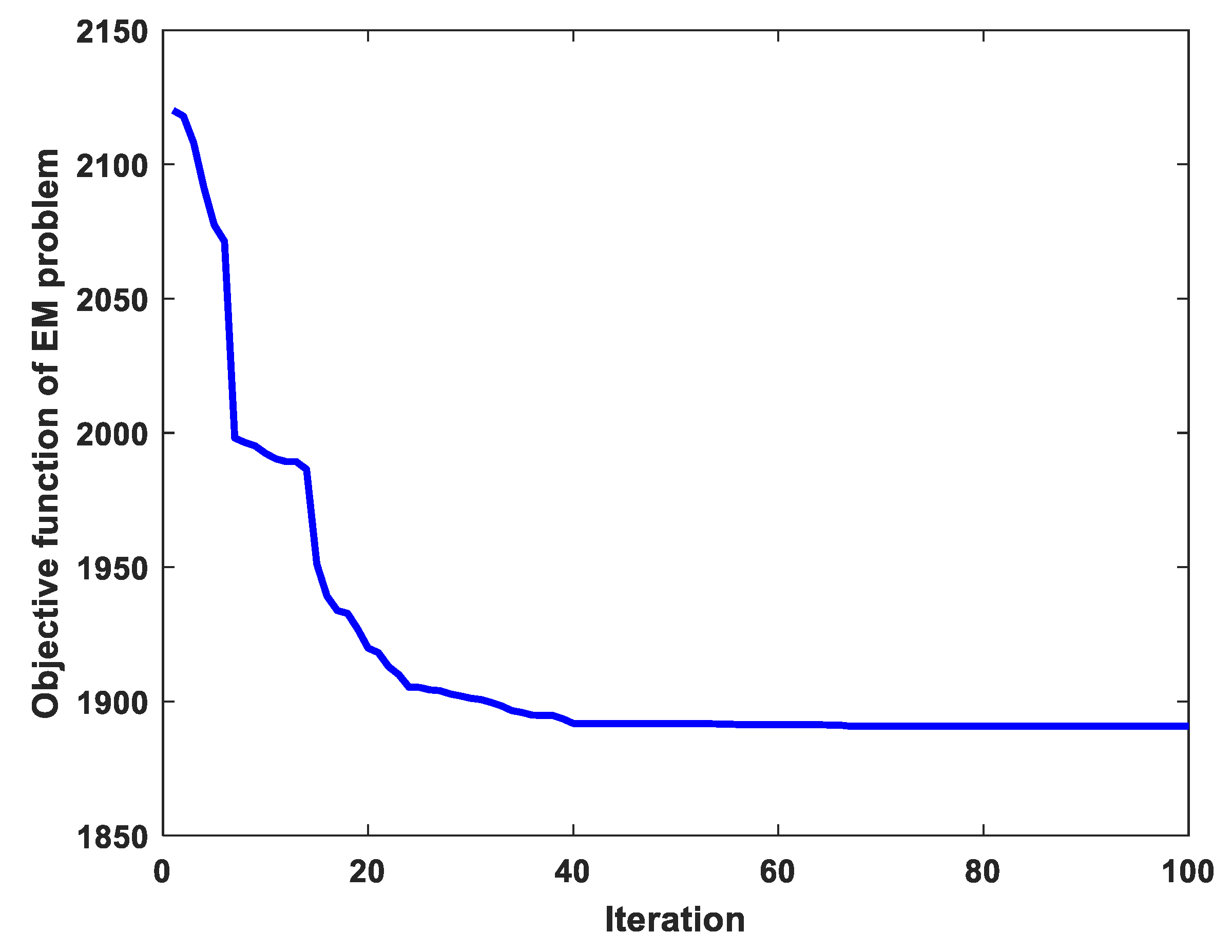
• Scenario 2: All MG sources are operated at their output power limits while satisfying operational constraints.
• Scenario 3: All MG sources except the main grid act as in Scenario 2, while the main grid is represented as an unconstrained source. Therefore, the energy will be exchanged without any limitations.

These scenarios are employed in the following cases studies.

5.1. Case 1: The Optimization of EM without Emission

In this case, the EO algorithm is implemented based on the first scenario for solving the EM deterministic optimization problem to minimize the total operating cost without considering the pullout emissions. The obtained results of the EO algorithm are compared with those results obtained from reported algorithms in [30,31]. All MG sources operate at each hour during the day, which means that the operator should buy at least the minimum output power generated from these sources. The initial charging of the battery is infinitive.

The simulation results obtained using the EO algorithm for Scenario 1 are tabulated in

Table 2. The best results obtained using EO for the energy management (EM) problem (Case 1).

Time (h)	Power (kW)						Cost
	PME-FC	MT	PV	WT	Battery	Utility	EUR/h
1	30.00	6.00	0.00	1.79	−15.79	30.00	14.38
2	30.00	6.00	0.00	1.79	−17.79	30.00	12.42
3	30.00	5.99	0.00	1.79	−17.61	29.91	10.94
4	30.00	6.00	0.00	1.79	−16.79	30.00	10.70
5	30.00	6.00	0.00	1.79	−11.79	30.00	12.60
6	30.00	6.00	0.00	0.92	−3.92	30.00	17.06
7	30.00	6.00	0.00	1.79	2.21	30.00	21.22
8	30.00	6.00	0.20	1.31	11.18	26.32	27.73
9	30.00	30.00	3.75	1.79	30.00	−19.54	16.23
10	30.00	30.00	7.53	3.09	30.00	−20.56	−25.96
11	30.00	28.78	10.45	8.78	30.00	−30.00	−50.21
12	30.00	21.96	11.95	10.41	30.00	−30.28	−48.87
13	30.00	14.19	23.90	3.92	30.00	−30.00	47.66
14	30.00	18.55	21.05	2.37	29.93	−29.86	−33.86
15	30.00	30.00	7.88	1.79	30.00	−23.66	8.87
16	30.00	30.00	4.23	1.31	30.00	−15.53	15.96
17	29.94	29.95	0.55	1.79	30.00	−7.23	32.89
18	30.00	6.00	0.00	1.79	30.00	20.22	33.17
19	30.00	6.00	0.00	1.30	22.64	30.10	32.08
20	30.00	6.00	0.00	1.79	30.00	19.21	33.14
21	30.00	30.00	0.00	1.30	30.00	−13.30	19.76
22	30.00	29.94	0.00	1.30	30.00	−20.21	24.36
23	30.00	5.97	0.00	0.92	−1.81	29.91	20.81
24	29.93	5.97	0.00	0.62	−10.65	30.14	15.98
Total operating cost (EUR)							269.07

. It is seen that because the PEM-FC unit has a lower bid compared to the other units, the PEM-FC operates at each hour of the day and delivers its maximum output power. In contrast, MT units which have a higher value of bid deliver their minimum value of output power for 13 h per day.

The results also show that, during the light load periods, a large part of the load is supplied by the main grid and PEM-FC because their bids are low. In addition, the battery was charged during this period. In contrast, in the periods of large load, the bid of the main grid is expensive, which required increasing the output power of MG. Additionally, the battery operates in discharge mode, and the excess energy from MG is exported to the main grid.

Further, 20 trial runs were performed for each algorithm for the purpose of comparing results and the simulation results as shown in

Table 3. Comparison of the EM problem based on Case 1.

Technique	Total Cost Function (EUR)
	Best	Worst	Mean	SD
EO	269.07025	269.303	269.1677	0.0937
ESSA (8)	269.7359	269.7359	269.7359	0
SGSA (25)	269.76	269.76	269.76	0
SSA (8)	270.9038	274.9021	272.4245	1.361
AMPSO-T (30)	274.4317	274.7318	274.5643	0.0921
AMPSO-L (30)	274.5507	275.0905	274.9821	0.321
CPSO-L (30)	274.7438	281.1187	276.3327	5.9697
CPSO-T (30)	275.0455	286.5409	277.4045	6.2341
GSA (25)	275.5369	282.1743	277.8021	2.9283
FSAPSO (30)	276.7867	291.7562	280.6844	8.3301
PSO (30)	277.3237	303.3791	288.8761	10.1821
GA (30)	277.7444	304.5889	290.4321	13.4421

. The results validate the effectiveness of the EO algorithm with the best value of the objective function when compared with the other techniques. Moreover, the convergence characteristic curve of the EO is shown in Figure 4, which demonstrates the robustness and fast convergence characteristic of the EO technique.

5.2. Case 2: The Optimization of EM with Emission Consideration

In this case, the deterministic EM problem is solved for minimizing the total objective function that includes minimizing emissions. The optimization problem is solved according to the mentioned previous three scenarios, and the results for each scenario are tabulated in

Table 4. The best results obtained using the EO for the EM problem for Scenario 1 (Case 2).

Time (h)	Power (kW)						Cost EUR/h	Emission Kg/h	Total Objective
	PME-FC	MT	PV	WT	Battery	Utility
1	3.00	6.00	0.00	1.79	30.00	11.22	23.42	23.65	40.75
2	3.00	6.00	0.00	1.79	30.00	9.22	22.43	23.24	41.57
3	3.00	6.00	0.00	1.79	29.93	9.30	21.85	22.97	40.27
4	3.00	6.00	0.00	1.79	30.00	10.22	21.82	23.07	41.30
5	3.00	6.00	0.00	1.79	30.00	15.22	22.52	23.27	38.76
6	3.00	6.00	0.00	0.92	30.00	23.09	24.75	24.67	67.08
7	3.00	6.00	0.00	1.79	30.00	29.26	28.40	25.76	44.74
8	7.54	6.00	0.20	1.31	30.00	30.00	35.60	36.12	77.05
9	29.94	29.97	3.75	1.79	30.00	−19.36	19.73	123.76	115.07
10	30.00	30.00	7.53	3.09	30.00	−20.62	−30.92	97.40	129.02
11	30.00	29.26	10.45	8.78	29.84	−30.33	−61.76	75.33	85.92
12	30.00	21.91	11.95	10.41	30.00	−30.27	−58.61	54.58	49.41
13	30.00	14.46	23.90	3.92	29.74	−30.02	57.14	71.92	110.05
14	29.97	18.60	21.05	2.37	29.97	−29.96	−41.04	46.44	34.36
15	30.00	30.00	7.88	1.79	29.79	−23.43	11.02	114.88	121.30
16	30.00	30.00	4.23	1.31	30.00	−15.53	19.16	123.49	143.79
17	16.66	6.00	0.55	1.79	30.00	30.00	48.45	55.88	138.00
18	20.21	6.00	0.00	1.79	30.00	30.00	41.16	59.39	107.73
19	22.97	6.00	0.00	1.30	30.00	29.82	39.26	62.98	117.39
20	19.24	6.00	0.00	1.79	30.00	30.00	41.53	57.81	127.01
21	30.00	6.19	0.00	1.30	30.00	10.59	44.14	76.90	146.46
22	3.00	6.71	0.00	1.30	30.00	30.00	39.39	31.72	50.12
23	3.00	6.00	0.00	0.92	30.00	25.09	28.24	26.12	34.76
24	3.00	6.00	0.00	0.62	30.00	16.39	23.93	24.49	35.43
Total cost (EUR)							421.60	-	-
Total emission (Kg)							-	1305.85	-
The total objective function (EUR)							-	-	1937.35

,

Table 5. The Best results obtained using EO for the EM problem for Scenario 2 (Case 2).

Time (h)	Power (kW)						Cost EUR/h	Emission Kg/h	Total Objective
	PME-FC	MT	PV	WT	Battery	Utility
1	3.00	6.00	0.00	1.78	30.00	11.22	21.47	20.84	42.33
2	3.00	6.00	0.00	0.00	30.00	11.01	18.83	20.56	46.90
3	3.00	6.00	0.00	0.00	30.00	11.00	18.22	20.39	45.53
4	3.00	6.00	0.00	0.00	30.00	12.00	18.11	20.34	45.28
5	3.00	6.00	0.00	0.00	30.00	17.00	18.77	20.61	46.82
6	3.00	6.00	0.00	0.00	30.00	24.00	21.81	21.82	33.95
7	3.00	6.00	0.00	1.78	30.00	29.22	26.02	22.66	43.02
8	7.90	6.00	0.10	1.30	30.00	29.70	32.62	31.98	85.01
9	29.98	29.94	2.75	1.79	30.00	−18.46	17.94	109.29	121.87
10	29.89	29.85	7.35	3.09	29.91	−20.03	−26.92	86.16	135.03
11	29.68	29.12	10.47	8.74	29.93	−29.93	−54.90	66.91	125.03
12	29.74	21.83	11.94	10.42	29.83	−29.76	−51.66	49.19	124.69
13	30.00	19.37	20.02	3.90	30.00	−31.22	51.16	63.50	162.06
14	30.00	18.59	21.04	2.37	30.00	−30.00	−37.80	41.11	33.71
15	30.00	30.00	7.79	1.79	30.00	−23.52	9.69	101.44	118.07
16	29.65	30.00	4.22	1.30	30.00	−15.12	16.63	109.03	139.06
17	16.71	6.00	0.55	1.79	30.00	30.00	44.42	49.34	31.59
18	20.22	6.00	0.00	1.78	30.00	30.00	37.73	52.47	41.91
19	22.70	6.00	0.00	1.30	30.00	30.00	35.98	55.63	52.90
20	19.27	6.00	0.00	1.78	29.95	30.00	38.09	50.91	104.20
21	29.89	6.00	0.00	1.31	29.80	10.99	40.84	68.28	70.55
22	3.00	6.70	0.00	1.30	30.00	30.00	36.11	27.95	97.71
23	3.00	6.00	0.00	0.91	30.00	25.09	25.88	23.02	73.09
24	3.00	6.00	0.00	0.00	30.00	17.00	21.96	21.51	63.95
Total cost (EUR)							381.02	-	-
Total emission (Kg)							-	1154.94	-
The total objective function (EUR)							-	-	1884.26

and

Table 6. The best results obtained using the EO for the EM problem for Scenario 3 (Case 2).

Time (h)	Power (kW)						Cost EUR/h	Emission Kg/h	Total Objective
	PME-FC	MT	PV	WT	Battery	Utility
1	3.00	6.00	0.00	1.78	30.00	11.22	19.52	20.37	38.68
2	3.00	6.00	0.00	0.00	30.00	11.01	17.15	20.24	38.09
3	3.00	6.00	0.00	0.00	30.00	11.00	16.60	19.96	38.53
4	3.00	6.00	0.00	0.00	30.00	12.00	16.52	20.00	39.39
5	3.00	6.00	0.00	0.00	30.00	17.00	17.08	20.13	42.83
6	3.00	6.00	0.00	0.00	30.00	24.02	19.84	21.33	48.44
7	3.00	6.00	0.00	0.00	30.00	31.00	23.66	22.15	58.11
8	3.00	6.00	0.00	1.30	30.00	34.70	29.61	24.93	65.77
9	30.00	30.00	3.75	1.79	30.00	−19.54	16.23	106.92	151.72
10	30.00	30.00	7.51	3.09	29.92	−20.52	−25.44	84.21	131.58
11	30.00	30.00	10.39	8.67	30.00	−31.06	−57.07	65.61	61.08
12	30.00	29.95	11.92	10.44	30.00	−38.30	−77.71	53.47	111.53
13	30.00	30.00	23.90	3.91	30.00	−45.82	31.17	89.97	107.93
14	30.08	29.95	21.04	2.36	29.97	−41.41	−74.80	48.30	120.36
15	29.99	29.81	7.83	1.79	30.00	−23.41	8.77	98.75	125.80
16	30.00	30.00	4.23	1.31	30.00	−15.53	15.96	106.50	150.65
17	3.00	6.00	0.55	1.78	30.00	43.67	44.56	30.53	55.14
18	3.00	6.00	0.00	1.79	30.00	47.22	36.30	27.58	55.99
19	3.00	6.00	0.00	1.30	30.00	49.70	33.82	26.74	50.38
20	3.00	6.00	0.00	1.78	30.00	46.22	36.80	27.77	60.35
21	30.00	6.00	0.00	1.30	30.00	10.72	36.88	66.66	60.94
22	3.00	6.00	0.00	1.30	30.00	30.70	33.00	26.39	54.12
23	3.00	6.00	0.00	0.91	30.00	25.09	23.53	22.50	48.19
24	3.00	6.00	0.00	0.61	30.00	16.40	19.94	21.07	38.41
Total cost (EUR)							261.90	-	-
Total emission (Kg)							-	1072.09	-
The total objective function (EUR)							-	-	1754.02

, respectively. The best results are achieved based on the EO algorithm; all operational constraints are also satisfied. In addition, Figure 5 shows the convergence characteristic of the EO algorithm for all scenarios in this case that validate the fast convergence characteristic of the EO method for all scenarios.

By inspecting the numerical results, during the period of light load, a large amount of load is supplied from the main grid and battery because these units offer both low bids and low emission as compared with other sources over these intervals. In the interval of heavy load, the output power from MTs and FCs is increased due to increasing bids through these intervals. Therefore, the main grid buys the energy from MG that assists in decreasing the cost of MG. From the results of the second scenario, the WT and PV are modeled for operating within their output power limits. The objective function is reduced by 2.74% when compared to the first scenario. Furthermore, when the main grid acts as an unconstrained source in the third scenario, the objective function is reduced by 9.46% and 6.91% as compared to the first and second scenarios, respectively. Due to the WT and PV having higher bids when compared with other MG sources, these sources have low contributions for supplying the demand load in the third scenario.

To prove the search capability and examine the superiority of the EO algorithm for solving the optimization problem in this case, the analysis is implemented for other recently published techniques to compare with the EO method. The compared methods are the artificial electric field algorithm (AEFA) [37], the bonobo optimizer (BO) [38], the modified moth flame optimization technique (MMFO) [39], and ESSA [8]. The results after 30 independent runs of EO are compared with AEFA, BO, MMFO, and ESSA. The statistical results are shown in

Table 7. Comparison of the statistical results of the objective function in Scenario 1.

	The Total Objective Function (EUR)
Technique	Best	Worst	Mean	(SD)
BO	1957.4649	1966.1141	1958.7819	2.3670
MMFO	1954.1966	1954.3167	1954.2005	0.0215
AEFA	1952.2123	1953.2124	1952.2447	0.1795
ESSA	1950.1667	1950.7642	1950.4	0.182
EO	1937.3514	1937.0698	1937.1736	0.0711

,

Table 8. Comparison of the statistical results of the objective function in Scenario 2.

	The Total Objective Function (EUR)
Technique	Best	Worst	Mean	(SD)
BO	1909.8416	1920.4749	1916.2545	2.6406
MMFO	1906.0516	1906.0516	1906.0516	0
AEFA	1899.8711	1907.9912	1904.9846	1.1588
ESSA	1896.416	1898.6641	1897.0065	0.3909
EO	1884.2562	1884.5921	1884.2969	0.0652

and

Table 9. Comparison of the statistical results of the objective function in Scenario 3.

	The Total Objective Function (EUR)
Technique	Best	Worst	Mean	(SD)
BO	1777.8915	1790.7626	1781.4435	3.5702
MMFO	1775.7734	1775.7734	1775.7734	0
AEFA	1770.261	1770.261	1770.261	0
ESSA	1769.2977	1769.2977	1769.2977	0
EO	1754.0217	1754.4085	1754.396	0.0694

for all considered scenarios, which reflect the satisfying performance of EO over other techniques that have the best value of the optimized objective function. It is seen that the EO has the best values of SD when compared with other techniques, which confirm the premium robustness of the EO technique.

Finally, due to the importance time for calculating this type of EM problem related to the computation of operating costs,

Table 10. The elapsed time (seconds) of Case 2 for all scenarios.

Technique	Scenarios
	Scenario1	Scenario 2	Scenario 3
BO	5.2416	6.1269	6.3516
MMFO	5.1465	5.3096	5.7125
AEFA	7.3665	7.7508	8.3447
ESSA	6.8463	7.3665	7.8508
EO	4.8704	5.2642	5.7147

displays the elapsed time of implementing all compared algorithms. It is seen that the EO takes a shorter time as compared to other algorithms for all three suggested scenarios.

5.3. Case 3: The Probabilistic EM Problem

In this case, for obtaining the optimal solution of the EM problem in the probabilistic frame, the point estimation method (2m + 1) is evaluated along with the EO algorithm and other compared techniques. Moreover, the output power generated from PV and WT, market price, and demand load level are adopted as uncorrelated random input variables. Utilizing proper PDF modeling for hourly data of solar irradiance and wind speed as described in Section 3.1.1 and Section 3.1.2, the output power of PV and WT units are computed. Additionally, the market price and demand load follow the same PDFs as given in Section 3.1.2. It is supposed that the output power of the PV and WT units, market price, and demand load have a normal distribution at an STD of 5% [10]. After that, the 2m + 1 method is employed, and the concentrations (locations) of the input random variables are calculated during the implementation of 2m + 1 for solving the probabilistic EM problem as displayed in

Table 11. The concentrations of the input variables used for EM problem in Case 3.

T (h)	PV1	PV2	WT1	WT2	Load1	Load2	MP1	MP2	$\mathbf{PV}\mathsf{\mu }$	$\mathbf{WT}\mathsf{\mu }$	$\mathbf{Load}\mathsf{\mu }$	$\mathbf{MP}\mathsf{\mu }$
1	0.00	0.00	1.91	1.60	56.45	47.23	0.25	0.21	0.00	1.79	51.92	0.23
2	0.00	0.00	1.90	1.61	54.48	45.32	0.21	0.17	0.00	1.78	50.00	0.19
3	0.00	0.00	1.91	1.55	54.07	45.74	0.15	0.13	0.00	1.78	49.93	0.14
4	0.00	0.00	1.92	1.55	55.37	46.73	0.13	0.11	0.00	1.79	51.04	0.12
5	0.00	0.00	1.91	1.59	60.98	51.06	0.13	0.11	0.00	1.79	55.97	0.12
6	0.00	0.00	0.98	0.81	68.60	57.69	0.22	0.18	0.00	0.92	63.07	0.20
7	0.00	0.00	1.91	1.58	75.82	63.95	0.25	0.21	0.00	1.78	70.01	0.23
8	0.22	0.18	1.40	1.17	81.66	68.81	0.41	0.35	0.20	1.31	75.12	0.38
9	4.06	3.43	1.91	1.57	82.32	69.07	1.63	1.37	3.74	1.78	76.17	1.49
10	8.12	6.94	3.30	2.75	86.75	73.91	4.33	3.64	7.53	3.09	80.24	4.00
11	11.32	9.54	9.41	7.80	84.81	71.61	4.34	3.64	10.45	8.78	78.02	4.00
12	13.03	10.83	11.10	9.38	80.44	67.03	4.36	3.63	12.93	10.40	73.82	4.00
13	26.03	21.80	4.19	3.49	78.11	65.89	1.64	1.38	24.91	3.92	72.09	1.50
14	22.97	19.14	2.52	2.13	78.56	66.05	4.36	3.66	21.14	2.37	72.19	4.01
15	8.58	7.16	1.91	1.56	82.33	69.00	2.17	1.84	7.89	1.82	75.97	2.00
16	4.65	3.85	1.40	1.15	86.58	73.12	2.11	1.78	4.6	1.30	79.70	1.95
17	0.60	0.50	1.91	1.56	92.26	78.31	0.65	0.55	0.55	1.78	85.21	0.60
18	0.00	0.00	1.92	1.56	94.85	80.46	0.44	0.38	0.00	1.79	87.73	0.41
19	0.00	0.00	1.38	1.19	97.68	82.03	0.38	0.32	0.00	1.30	89.94	0.35
20	0.00	0.00	1.91	1.58	94.68	79.89	0.47	0.39	0.00	1.79	87.09	0.43
21	0.00	0.00	1.39	1.16	84.51	71.34	1.28	1.07	0.00	1.30	77.84	1.17
22	0.00	0.00	1.39	1.15	77.34	64.64	0.59	0.49	0.00	1.30	71.00	0.54
23	0.00	0.00	0.98	0.81	70.47	59.67	0.33	0.27	0.00	0.92	64.95	0.30
24	0.00	0.00	0.66	0.55	60.60	51.27	0.28	0.24	0.00	0.61	56.04	0.26

. The EO algorithm and other compared techniques are applied for each case data results obtained from (2m + 1) as presented in Table 11. Finally, the statistical moments, mean values, and STD of the EM output random variables (the operating cost of MG) are determined.

Only the second scenario is considered in this case, where all MG sources are represented within their power limits. The predictable output power generated from MG sources and the corresponding cost based on EO algorithm are obtained using the mean values of the random input variables as displayed in Table 11 (the last four columns). The best simulation results of the EO algorithm are shown in

Table 12. The best results obtained using the EO for the EM problem in Case 3.

Time (h)	Power (kW)						Cost EUR/h	Emission Kg/h	Total Objective
	PME-FC	MT	PV	WT	Battery	Utility
1	3.00	6.00	0.00	1.00	30.00	12.00	19.50	20.36	32.84
2	3.00	6.00	0.00	0.00	30.00	11.00	17.12	20.16	35.64
3	3.00	6.00	0.00	0.00	30.00	11.00	16.55	19.93	34.23
4	3.00	6.00	0.00	0.00	29.87	12.13	16.44	19.92	33.98
5	3.00	6.00	0.00	0.00	29.90	17.10	17.05	20.14	35.48
6	3.00	6.00	0.00	0.00	30.00	24.00	20.03	21.45	33.01
7	3.00	6.00	0.00	1.78	30.00	29.22	23.65	22.15	71.31
8	7.50	6.00	0.20	1.31	30.00	30.00	29.68	31.33	62.94
9	30.00	30.00	3.57	1.78	30.00	−19.35	16.60	107.04	129.41
10	30.00	30.00	7.29	3.09	30.00	−20.38	−24.80	84.47	30.43
11	30.00	28.80	10.42	8.78	30.00	−30.00	−50.34	65.00	42.24
12	30.00	21.53	12.22	10.40	29.91	−30.06	−47.99	47.35	54.54
13	30.00	14.28	23.89	3.83	30.00	−30.00	47.57	61.95	130.41
14	30.00	18.69	21.11	2.37	30.12	−30.28	−35.34	40.39	35.76
15	30.00	30.00	7.88	1.80	29.72	−23.40	8.86	99.69	115.97
16	30.00	30.00	4.52	1.30	30.00	−15.82	15.39	106.26	126.11
17	17.03	6.00	0.55	1.77	30.00	29.65	40.38	48.77	122.44
18	20.21	6.00	0.00	1.79	30.00	30.00	34.19	50.86	90.48
19	22.70	6.00	0.00	1.30	30.00	30.00	32.67	54.27	80.61
20	19.13	6.00	0.00	1.77	30.00	30.09	32.23	49.88	116.40
21	30.00	6.00	0.00	1.30	30.00	10.70	36.69	66.49	141.98
22	3.70	6.00	0.00	1.30	30.00	30.00	51.71	27.31	135.18
23	3.00	6.00	0.00	0.92	30.00	25.03	45.28	22.49	117.05
24	3.00	6.00	0.00	0.61	30.00	16.31	19.97	20.91	82.37
Total cost (EUR)							383.09	-	-
Total emission (Kg)							-	1128.55	-
The total objective function (EUR)							-	-	1890.79

, which shows that all operational constraints are met. However, the convergence curve of EO for this case is shown in Figure 6, in which the results indicate to the fast convergence characteristic of EO. It is seen that, during light load periods, the produced energy is supplied from the main grid and battery, causing these sources to have lower market prices and lower emissions when compared with other sources over these periods. Additionally, the contributions of PV and WT are lower than other sources because these units have a higher market price.

Using the Gram–Charlier expression for series expansion of the obtained results based on solving EM using the EO along with the two locations of each input random variables, the PDFs and CDFs are obtained for the optimal solutions of the probabilistic EM as shown in Figure 7. It is clear that there is no difference between the continuous random variables and the normal distributions as seen in Figure 7, which also shows that the EO algorithm gives the best results in the case of solving the EM in a probabilistic manner.

The superiority of the EO is inspected here over the stated previous techniques in the previous subsection.

Table 13. Comparison of the statistical results of the objective function in Case 3.

	The Total Objective Function (EUR)
Technique	Best	Worst	Mean	(SD)
BO	1916.9103	1925.9192	1922.802	1.8102
MMFO	1918.2695	1918.8269	1918.3043	0.1350
AEFA	1909.8144	1912.3462	1910.3477	0.4595
ESSA	1901.6784	1901.6784	1902.1042	0.1263
EO	1890.7867	1890.9909	1890.8905	0.0439

shows the statistical results of 30 independent runs of the EO algorithm compared with AFEA, BO, MMFO, and ESSA. The results of the proposed EO for solving probabilistic EM show that the EO has better effectiveness and performance in comparison with other techniques. Additionally, the EO has premium robustness due to having a lower value of SD compared with other techniques. Moreover, the superiority of the EO is inspected here over the stated previous techniques in the previous subsection.

By analyzing the results for Cases 2 and 3 based on Scenario 2, the total objective function is increased in Case 3 due to considering the impact of uncertainty when solving the optimization problem. This proves the impact of considering the uncertainty of input variables of the EM problem and the decision making of operators because the probabilistic analysis of EM gives more accurate and trustworthy results.

6. Conclusions

An efficient EO algorithm was suggested in this paper with successful implementation to solve the EM optimization problem for a typical MG system. Furthermore, the probabilistic framework using the 2m + 1 method was proposed to model the uncertainties of input random variables. The proposed EO was utilized for finding the optimal solution of EM incorporating ES devices, considering the emissions of MG sources based on converting the multi-objective function using the penalty factor price to the single objective function to minimize the total operating costs (fuel cost, startup and shutdown cost, as well as emission cost). The efficiency and advantages of the EO have been proven using a standard MG test system operating in grid-connected mode with different operating scenarios of the deterministic and probabilistic EM problem. Solving EM based on a probabilistic approach provided useful realistic decision making for operators of the MG system and assisted in finding the impact of the uncertainties for the input random variables on the statistical indicators which describe the state of the MG system. It was confirmed that the total operating cost for Scenario 2 based on probabilistic EM had higher value than deterministic EM by 6.53 EUR (0.346%) per day. The results confirm smooth and reliable EO convergence without any oscillation in the response. This confirmed the superiority of the EO over other compared optimization algorithms. In this context, the EO could be a useful decision-making tool for operators in the MG control center.

References

1. Zia, M.F.; Elbouchikhi, E.; Benbouzid, M. Microgrids energy management systems: A critical review on methods, solutions, and prospects. Appl. Energy 2018, 222, 1033–1055. [Google Scholar] [CrossRef]
2. Moradi, H.; Esfahanian, M.; Abtahi, A.; Zilouchian, A. Optimization and energy management of a standalone hybrid microgrid in the presence of battery storage system. Energy 2018, 147, 226–238. [Google Scholar] [CrossRef]
3. Khan, A.A.; Naeem, M.; Iqbal, M.; Qaisar, S.; Anpalagan, A. A compendium of optimization objectives, constraints, tools and algorithms for energy management in microgrids. Renew. Sustain. Energy Rev. 2016, 58, 1664–1683. [Google Scholar] [CrossRef]
4. Li, X.; Zhang, R.; Bai, L.; Li, G.; Jiang, T.; Chen, H. Stochastic low-carbon scheduling with carbon capture power plants and coupon-based demand response. Appl. Energy 2018, 210, 1219–1228. [Google Scholar] [CrossRef]
5. Liu, G.; Jiang, T.; Ollis, T.B.; Zhang, X.; Tomsovic, K. Distributed energy management for community microgrids considering network operational constraints and building thermal dynamics. Appl. Energy 2019, 239, 83–95. [Google Scholar] [CrossRef]
6. Hirsch, A.; Parag, Y.; Guerrero, J. Microgrids: A review of technologies, key drivers, and outstanding issues. Renew. Sustain. Energy Rev. 2018, 90, 402–411. [Google Scholar] [CrossRef]
7. Tabatabaee, S.; Mortazavi, S.S.; Niknam, T. Stochastic energy management of renewable micro-grids in the correlated environment using unscented transformation. Energy 2016, 109, 365–377. [Google Scholar] [CrossRef]
8. Elattar, E.E.; ElSayed, S.K. Probabilistic energy management with emission of renewable micro-grids including storage devices based on efficient salp swarm algorithm. Renew. Energy 2020, 153, 23–35. [Google Scholar] [CrossRef]
9. Serraji, M.; El Amine, D.O.; Boumhidi, J. Multi swarm optimization based adaptive fuzzy multi agent system for microgrid multi-objective energy management. Int. J. Knowl. Based Intell. Eng. Syst. 2016, 20, 229–243. [Google Scholar] [CrossRef]
10. Radosavljević, J. Metaheuristic Optimization in Power Engineering; Institution of Engineering and Technology: London, UK, 2018. [Google Scholar]
11. Aghajani, G.; Ghadimi, N. Multi-objective energy management in a micro-grid. Energy Rep. 2018, 4, 218–225. [Google Scholar] [CrossRef]
12. Mellouk, L.; Ghazi, M.; Aaroud, A.; Boulmalf, M.; Benhaddou, D.; Zine-Dine, K. Design and energy management optimization for hybrid renewable energy system-case study: Laayoune region. Renew. Energy 2019, 139, 621–634. [Google Scholar] [CrossRef]
13. Liu, G.; Ollis, T.B.; Zhang, Y.; Jiang, T.; Tomsovic, K. Robust Microgrid Scheduling with Resiliency Considerations. IEEE Access. 2020, 8, 153169–153182. [Google Scholar] [CrossRef]
14. Jafari, M.; Malekjamshidi, Z. Optimal energy management of a residential-based hybrid renewable energy system using rule-based real-time control and 2D dynamic programming optimization method. Renew. Energy 2020, 146, 254–266. [Google Scholar] [CrossRef]
15. Liu, C.; Wang, X.; Wu, X.; Guo, J. Economic scheduling model of microgrid considering the lifetime of batteries. IET Gener. Transm. Distrib. 2017, 11, 759–767. [Google Scholar] [CrossRef]
16. Guo, L.; Liu, W.; Jiao, B.; Hong, B.; Wang, C. Multi-objective stochastic optimal planning method for stand-alone microgrid system. IET Gener. Transm. Distrib. 2014, 8, 1263–1273. [Google Scholar] [CrossRef]
17. Kuznetsova, E.; Ruiz, C.; Li, Y.; Zio, E. Analysis of robust optimization for decentralized microgrid energy management under uncertainty. Int. J. Electr. Power Energy Syst. 2015, 64, 815–832. [Google Scholar] [CrossRef]
18. Marzband, M.; Yousefnejad, E.; Sumper, A.; Domínguez-García, J.L. Real time experimental implementation of optimum energy management system in standalone microgrid by using multi-layer ant colony optimization. Int. J. Electr. Power Energy Syst. 2016, 75, 265–274. [Google Scholar] [CrossRef] [Green Version]
19. Marzband, M.; Azarinejadian, F.; Savaghebi, M.; Guerrero, J.M. An optimal energy management system for islanded microgrids based on multiperiod artificial bee colony combined with Markov chain. IEEE Syst. J. 2015, 11, 1712–1722. [Google Scholar] [CrossRef] [Green Version]
20. Nikmehr, N.; Najafi-Ravadanegh, S. Optimal operation of distributed generations in micro-grids under uncertainties in load and renewable power generation using heuristic algorithm. IET Renew. Power Gener. 2015, 9, 982–990. [Google Scholar] [CrossRef]
21. Wang, H.; Huang, J. Joint investment and operation of microgrid. IEEE Trans. Smart Grid 2015, 8, 833–845. [Google Scholar] [CrossRef] [Green Version]
22. Arabali, A.; Ghofrani, M.; Etezadi-Amoli, M.; Fadali, M.S.; Baghzouz, Y. Genetic-algorithm-based optimization approach for energy management. IEEE Trans. Power Deliv. 2012, 28, 162–170. [Google Scholar] [CrossRef]
23. Radosavljević, J.; Jevtić, M.; Klimenta, D. Energy and operation management of a microgrid using particle swarm optimization. Eng. Optim. 2016, 48, 811–830. [Google Scholar] [CrossRef]
24. Niknam, T.; Golestaneh, F.; Malekpour, A. Probabilistic energy and operation management of a microgrid containing wind/photovoltaic/fuel cell generation and energy storage devices based on point estimate method and self-adaptive gravitational search algorithm. Energy 2012, 43, 427–437. [Google Scholar] [CrossRef]
25. Niknam, T.; Golestaneh, F.; Shafiei, M. Probabilistic energy management of a renewable microgrid with hydrogen storage using self-adaptive charge search algorithm. Energy 2013, 49, 252–267. [Google Scholar] [CrossRef]
26. Mohammadi, S.; Mozafari, B.; Solimani, S.; Niknam, T. An Adaptive Modified Firefly Optimisation Algorithm based on Hong’s Point Estimate Method to optimal operation management in a microgrid with consideration of uncertainties. Energy 2013, 51, 339–348. [Google Scholar] [CrossRef]
27. Afshin, F.; Mohammad, H.; Brent, S. Equilibrium optimizer: A novel optimization algorithm. Knowl. Based Syst. 2019, 191, 105190. [Google Scholar]
28. Agnihotri, S.; Atre, A.; Verma, H.K. Equilibrium Optimizer for Solving Economic Dispatch Problem. In Proceedings of the IEEE 9th Power India International Conference (PIICON), Delhi, India, 28 February–1 March 2020. [Google Scholar]
29. Menesy, A.S.; Sultan, H.M.; Kamel, S. Extracting Model Parameters of Proton Exchange Membrane Fuel Cell Using Equilibrium Optimizer Algorithm. In Proceedings of the International Youth Conference on Radio Electronics, Electrical and Power Engineering (REEPE), Moscow, Russia, 12–14 March 2020. [Google Scholar]
30. Moghaddam, A.A.; Seifi, A.; Niknam, T.; Pahlavani, M.R.A. Multi-objective operation management of a renewable MG (micro-grid) with back-up micro-turbine/fuel cell/battery hybrid power source. Energy 2011, 36, 6490–6507. [Google Scholar] [CrossRef]
31. Niknam, T.; Golestaneh, F. Enhanced adaptive particle swarm optimisation algorithm for dynamic economic dispatch of units considering valve-point effects and ramp rates. IET Gener. Transm. Distrib. 2012, 6, 424–435. [Google Scholar] [CrossRef]
32. Bouchekara, H.; Abido, M.A.; Boucherma, M. Optimal power flow using teaching-learning-based optimization technique. Electr. Power Syst. Res. 2014, 114, 49–59. [Google Scholar] [CrossRef]
33. Krishnamurthy, S.; Tzoneva, R. Impact of price penalty factors on the solution of the combined economic emission dispatch problem using cubic criterion functions. In Proceedings of the IEEE Power and Energy Society General Meeting, San Diego, CA, USA, 22–26 July 2012. [Google Scholar]
34. Villanueva, D.; Pazos, J.L.; Feijo, A. Probabilistic load flow including wind power generation. IEEE Trans. Power Syst. 2011, 26, 1659–1667. [Google Scholar] [CrossRef]
35. Atwa, Y.M.; El-Saadany, E.F.; Salama, M.M.A.; Seethapathy, R.; Assam, M.; Conti, S. Adequacy evaluation of distribution system including wind/solar DG during different modes of operation. IEEE Trans. Power Syst. 2011, 26, 1945–1952. [Google Scholar] [CrossRef]
36. Zhang, P.; Lee, S.T. Probabilistic load flow computation using the method of combined cumulants and Gram-Charlier expansion. IEEE Trans. Power Syst. 2004, 19, 676–682. [Google Scholar] [CrossRef]
37. Yadav, A. AEFA: Artificial electric field algorithm for global optimization. Swarm Evol. Comput. 2019, 48, 93–108. [Google Scholar]
38. Das, A.K.; Pratihar, D.K. A new bonobo optimizer (BO) for real-parameter optimization. In Proceedings of the 2019 IEEE Region 10 Symposium (TENSYMP), Kolkata, India, 7–9 June 2019. [Google Scholar]
39. Elattar, E.E.; Elsayed, S.K. Optimal Location and Sizing of Distributed Generators Based on Renewable Energy Sources Using Modified Moth Flame Optimization Technique. IEEE Access 2020, 8, 109625–109638. [Google Scholar] [CrossRef]
Figure 1. One-line diagram of a standard micro-grid (MG) test system.
Energies 14 01373 g001
Figure 2. Flowchart of the equilibrium optimizer (EO) algorithm.
Energies 14 01373 g002
Figure 3. (a) Forecasted demand load; (b) bid coefficients of MG sources; (c) the output power from photovoltaics (PV); (d) wind turbines (WT).
Energies 14 01373 g003
Figure 4. Convergence characteristic of EO for Case 1.
Energies 14 01373 g004
Figure 5. Convergence characteristic of the EO for all scenarios in Case 2.
Energies 14 01373 g005
Figure 6. Convergence characteristic of the EO for Case 3.
Energies 14 01373 g006
Figure 7. (a) Probability density function (PDF); (b) cumulative density function (CDF) of forecasted objective function based on the EO for Case 3.
Energies 14 01373 g007