Multiple Solutions of the Tristable Energy Harvester

Abstract

This paper presents the results of numerical simulations of a non-linear, tristable system for harvesting energy from vibrating mechanical devices. Detailed model tests were carried out in relation to the system consisting of a beam and three permanent magnets. Based on the derived mathematical model and assuming a range of control parameter variability, a three-dimensional image of the distribution of the largest Lyapunov exponent was plotted. On its basis, the regions of chaotic and predictable movement of the considered system exist have been established. With reference to selected plane of the largest Lyapunov exponent cross-sections, possible co-existing solutions were identified. To identify multiple solutions, a diagram of solutions (DS) diagram was used to illustrate the number of existing solutions and their periodicity. The proposed calculation tool is based on the so-called fixed points of Poincaré cross-section. In relation to selected values of the control parameter ω, coexisting periodic solutions were identified for which phase trajectories and basins of attraction were presented. Based on the model tests carried out, it was found that in order to efficiently harvest energy, appropriate transducer adjustment is required. Calibration of the transducer is necessary to obtain the greatest amplitude of vibration of the beam, which corresponds to the phase trajectory limited by external energy potential barriers. As expected, the average voltage induced on the electrodes of the piezoelectric transducer and the average electrical power recorded on the resistive element are directly proportional to the amplitude and average kinetic energy of the beam.

1. Introduction

In most machine design solutions, induced mechanical vibrations are considered to be unfavourable because their presence reduces reliability and durability, which in turn leads to shorten service life, economic losses, and, in extreme cases, equipment failure or destruction. Cyclic dynamic loads of a certain intensity also adversely affect the comfort of people operating machinery [1,2]. Most practical applications minimize their impact through passive and active vibration reduction systems. On the other hand, some machines are constructed where cyclic loads are intentionally induced. The increasing demand for energy lead to research focussed on the development of new technologies for alternative power sources. Currently, there is a tendency to replace energy from fossil fuels or nuclear sources with renewable sources based on wind [3,4] water, [5] or solar radiation [6]. In the case of low power, an alternative is to obtain electricity from vibrating mechanical systems via electrostatic [7], electromagnetic [8] and piezoelectric transducers [9,10]. They are not energy-efficient sources, but the energy obtained in this way is sufficient to power simple electronic systems or sensors that remotely monitor the operation of the machine [11]. These transducers fulfil their tasks more effectively if their resonance frequency is optimally tuned to the frequency of the vibrating device [12,13]. The overwhelming majority of new solutions are based on nonlinear resonators [14]. Various nonlinear effects were discussed and utilised [15,16]. One of proposed systems is based on piezoelectric transducers are designed around a system consisting of a flexible beam with magnets and two permanent magnets, located symmetrically near its free end [17,18]. Magnets modify the system’s stiffness and lead to a double-well potential. As a result, the resonance area is expanded and additional solutions are obtained [19,20,21,22]. Since multiple resonant frequencies can be excited during machine operation, research was carried performed implementing multiple transducers connected in parallel, each of which was tuned to a different frequency [23]. A similar idea was used in the work [24] in which two magnetopiezoelastic oscillators coupled with an electric circuit were analysed. In this case, the extension of the synchronization condition for a non-linear system was used.

Research on harvesting energy from vibrating mechanical devices is gaining interest. In particular, systems based on the Duffing equation, with two stable equilibrium positions—bistable energy harvesters (BEH), characterized by a short transition time between various stable mechanical states, and thus being able to cause motion of considerable amplitude. Their non-linear characteristics mean that the efficiency of energy harvesting increases significantly due to the excited harmonics over a wide frequency range [25]. In relation to bistable randomly excited systems, a reduction in energy harvesting is observed. The introduction of an additional small permanent magnet, located between the main magnets allows for the modification of the potential barrier, while ensuring an unstable position of the beam in the middle position—this arrangement is referred to as the improved bistable energy harvester (IBEH). This modification facilitates oscillations between potential wells which results in transitions at fairly low excitation [26]. In order to improve the efficiency of energy converters, at low excitation amplitudes, Zhou et al. [27] proposed a system having three potential wells induced by a magnetic field—this arrangement is referred to as the tristable energy harvester (TEH). The results of modelling and experimentation of such a construction indicates that TEH performance exceeds that of the BEH [28,29,30,31]. Whereas in the work [32] a TEH was subjected to model tests, in which energy potential wells are asymmetrically distributed. Based on the results, it was found that such a system of energy harvesting has four stable solutions. Results show that the potential barrier plays an essential role in periodic inter-wells orbits which results in an increased voltage potential at the transducer.

By introducing additional permanent magnets and configuring them in an appropriate way, it is possible to shape the potential barrier. In the paper [33] a system consisting of a beam with a magnet at its end, and four permanent magnets located on the base was examined. In order to achieve the best stability, the permanent magnets were mounted on two inclined surfaces, resulting in five stable equilibrium (pentastable energy harvester—PEH) positions. With regard to the BEH, PEHs are characterized by shallower wells, which makes it easier to achieve movement between wells with high amplitude. In parallel with experimental research [34], theoretical works [35] are also carried out in the field of dynamics of multi-stable piezoelectric transducers. System solutions with five wells were tested by analytically approximate methods [36]. Using the Lindstedt-Poincaré method and the approximation of multiple time scales, the authors found eleven different system responses when the excitation amplitude changed.

From a technical point of view, the design of most systems for energy harvesting from vibrating mechanical systems is based on a flexible beam and permanent magnets. This group includes the transducers mentioned previously. A similar solution was used in the work [37], nevertheless the proposed system uses limiters for flexible beam movement. Wang et al. concluded that their system design allows for an almost 35-fold increase in energy harvesting compared to a conventional method. There are also solutions where the movement of two flexible beams is coupled via a spring [38]. Another concept for energy harvesting is presented in [39], where two beams with glued transducers are inertially coupled, as a result of which piezoelectrics are affected by components resulting from bending of beams and fluctuations of the inertial coupling mass. This solution is characterized by two resonance frequencies, which results in increased frequency bandwidth and, as a consequence, more efficient energy harvest is possible compared to design solutions with only one natural frequency.

Bearing in mind the review of the latest achievements, model research was undertaken to evaluate the solutions of multiple non-linear dynamic systems for the efficiency of energy harvesting. In particular, focus was placed on assessing the sensitivity of initial conditions to the nature of the system response, which was depicted in the form of phase trajectories and basins of attraction. To carry out such model tests, an original approach based on a diagram of multiple solutions (DMS) was used.

Chaos theory has many tools that can be used to identify zones of chaotic movement. In addition to commonly implemented methods such as: Poincaré cross-section [40,41], the largest Lyapunov exponent [42,43], bifurcation diagrams [44], test 0–1 [45,46], you can use relatively unknown tools such as diagrams of the number of phase stream intersections (NPSI) or a correlation dimension [47]. However, these methods are not capable of determining the number of co-existing solutions and the nature of the solution. Identification of multiple solutions and their periodicity requires the use of other procedures and additional numerical tests.

In fact, the DMS diagram is a combination of two charts representing periodicity of solutions and the number of solutions. The basic purpose of the DMS diagram is to recognize and search for stable periodic solutions. In general terms, the method is used to identify the so-called fixed points of phase streams, whose origins are located at various points of the studied area of the phase plane. We focused our attention on a system with three wells, whose characteristics, reflecting the cause-effect relationships between permanent magnets, were recorded under laboratory conditions.

2. Formulation of Computational Models

The subject of research is system for energy harvesting from vibrating mechanical systems, based on a flexible beam I (Figure 1). Its mechanical features were reflected by the stiffness c_B and the viscous damper b_B. These parameters were identified on the basis of geometric dimensions: length L = 101 mm, width d = 15 mm and thickness h = 0.27 mm and elastic properties of the material given by Young modulus E = 2.1 × 10¹¹ Pa. In addition, we assume a priori their linear mechanical characteristics and any nonlinearities occurring in the examined systems are caused by interactions occurring between permanent magnets. Additionally, the dissipative element takes into account energy losses due to deformation and friction at the point of attachment to the rigid non-deformable frame III.

A piezoelectric transducer II is glued onto the beam, which generates an electric charge as a result of the elastic deformation of the beam. Frame III, via mounting screws IV, creates a fixed connection with the vibrating mechanical system. In addition, in the frame III, permanent magnets are fixed, which are arranged symmetrically with respect to the axis of the vibrating beam.

Based on the formulated phenomenological model, differential motion equations were derived, enabling quantitative and qualitative model studies. During computer simulations, kinematic excitation was assumed, reflected by harmonic function $q_1=Asin\left({\omega }_{W}t\right)$. Equations of motion, engaging electromechanical coupling take the form:

$$\{\begin{array}{l}{m}_1\frac{d^2{q}_2}{d{t}^2}+b_B\left(\frac{d{q}_2}{dt}-\frac{d{q}_1}{dt}\right)+c_B\left(q_2-q_1\right)+F_M+k_P{U}_P=0,\hfill \\ C_P\frac{d{U}_P}{dt}+\frac{U_P}{R_O}-k_P\left(\frac{d{q}_2}{dt}-\frac{d{q}_1}{dt}\right)=0.\hfill \end{array}$$

(1)

here m₁ represents the mass of the magnet loading the beam I (Figure 1), q₂ corresponds to the vertical displacement of mass m₁, while F_M value represents the impact of electromagnetic loads, mapping the cause-effect relationships between magnetic forces and beam displacements. During numerical experiments, they are most often mapped to a polynomial function [36]. In our case, its general representation takes the form: $F_M=c_{1}x+c_2{x}^3+c_3{x}^5$. Bearing in mind the values listed in

Table 1. Physical parameters of energy harvesting systems.

Parameter	Symbol	Value
Concentrated mass loading the beam	m1	0.0032 kg
Energy losses in a mechanical system	bB	0.0105 Nsm−1
Beam stiffness	cB	0.05 Nm−1
Equivalent resistance of the electrical circuit	RO	1.0 × 106 Ω
Electrical circuit equivalent capacity	CP	72 nF
Electromechanical constant of piezoelectric	kP	3.985 × 10−5 N/V

, the bending beam stiffness was estimated based on the equation c_B = EI_B/L, where I_B represents the moment of inertia of the beam section. The formal basis for conducting computer simulations are non-linear differential equations. For this purpose, we introduce a new variable defined as the displacement difference $x=q_2-q_1$. Below we assume that A and x are expressed in [m]:

$$\{\begin{array}{l}{m}_1\frac{d^{2}x}{d{t}^2}+b_B\frac{dx}{dt}+c_{B}x+c_{1}x+c_2{x}^3+c_3{x}^5+k_P{U}_P={\omega }_W^2{m}_{1}Asin\left({\omega }_{W}t\right),\hfill \\ C_P\frac{d{U}_P}{dt}+\frac{U_P}{R_O}-k_P\frac{du}{dt}=0.\hfill \end{array}$$

(2)

Model tests in the scope of quantitative and qualitative assessment of non-linear dynamics of the system for energy harvesting from mechanical vibrations, differential Equation (2) have been transformed into the following form, whereby the new generalized coordinate depends on dimensionless time $\tau ={\omega }_{0}t$:

$$\{\begin{array}{l}\ddot{x}+\delta \dot{x}+x+\alpha x^3+\beta x^5+\theta U_P={\omega }^{2}Asin\left(\omega \tau \right),\hfill \\ {\dot{U}}_P+\sigma U_P-\vartheta \dot{x}=0.\hfill \end{array}$$

(3)

where:

$$\begin{array}{c}{\omega }_0^2=\frac{c_B+c_1}{m_1},\omega =\frac{{\omega }_W}{{\omega }_0},\delta =\frac{b_B}{m_1{\omega }_0},\alpha =\frac{c_2}{c_1},\beta =\frac{c_3}{c_1},\\ \theta =\frac{k_P}{m_1{\omega }_0^2},\vartheta =\frac{k_P}{C_P},\sigma =\frac{1}{C_P{R}_O{\omega }_0}.\end{array}$$

This paper presents the results of numerical calculations of the TEH system. Registered in experimental research measurement data presented by Zhou et al. [27] were approximated by a polynomial function and characteristic coefficients were identified F_M: c₁ ≈ 3.818, c₂ ≈ −48,931, c₃ ≈ 1.12 × 10⁸. On this basis, the potential function was defined, in the form of total energy:

$$E=\frac{{\dot{x}}^2}{2}+\frac{x^2}{2}+\frac{\alpha x^4}{4}+\frac{\beta x^6}{6}.$$

(4)

Derived equations of motion (3) are the formal basis for conducting model tests of energy harvesting systems.

3. Model Tests Results

Model studies were carried out in relation to the energy harvesting system, for which the energy potential is described by three wells. We assume that the system is affected by the harmonic excitation with amplitude A and frequency ω_W. The stiffness of the beam was calculated on the beam dimensions and material. Since the system being considered is non-linear, and is sensitive to small changes in parameters [48], the stiffness of the beam will be considered even though its contribution is small relative to F_M. Note that the beam as a mechanical system works within the Hooke’s law. In this range, it does not undergo plastic deformation, therefore its mechanical characteristics are linear. Nevertheless, the influence of the directional coefficient of the mechanical characteristic, which is determined by the geometry of the beam and the material properties, is so small in relation to the interaction caused by the magnets that it could be ignored. Nevertheless, taking into account the sensitivity of nonlinear systems to small changes in parameters, it was decided to include it in the mathematical model. Additionally, the cause-and-effect relations between the magnets embedded in the frame and the magnet mounted on the beam have been recorded in laboratory conditions. The F_M characteristic, taking into account the influence of the beam linear stiffness, was also recorded in laboratory conditions. The numerical values characterizing the tested system, necessary to perform computer simulations, are presented in Table 1.

A three-dimensional distribution map of the largest Lyapunov exponent was generated and periodic motion zones were identified [49]. It is possible to determine the speed of separation initially infinitely close trajectories. If the system exhibits chaotic behaviour, then the distance between trajectories increases exponentially over time. Chaotic motion occurs when the value of the largest Lyapunov exponent λ has positive values λ > 0. However, the predictable periodic motion occurs when λ < 0. In our research, we estimated the largest Lyapunov exponent based on the formula given by the equation:

$$\lambda =\underset{\epsilon \left(0\right)\to 0,n\to \infty }{\lim }\frac{1}{n \tau }{\displaystyle \sum }_{i=1}^{n}ln\left(\frac{{\epsilon }_i\left(\tau \right)}{\epsilon \left(0\right)}\right).$$

(5)

In the above equation ε_i(τ) represents the vectors that link, at the same moment of time, the trajectory of the studied motion with the reference trajectory. At the moment τ = 0, the beginnings of both phase streams are located in close proximity, and the distance between them on the phase plane defines the parameter ε(0) = 10⁻⁵. In practical applications, the calculation procedure is reduced to averaging after many iterations, in an adequate immersion space. In Equation (5), n corresponds to the number of averaged phase trajectories. Due to the linear coupling of the mechanical resonator with the electric circuit, we have adopted a reduced phase space for the exponent calculations, defined by the displacement and velocity of the beam end $\left(u,\dot{u}\right)$. In order to obtain satisfactory resolution, it is necessary to carry out multiple numerical simulations that prolong the calculation time. Acceptable resolution was obtained by dividing the ranges of variability of control parameters ω and A into 500 intervals, to which abscissa and ordinate axes were assigned. As a result of these assumptions, 250,000 computer simulations were performed to generate a single three-dimensional diagram of the largest Lyapunov exponent.

On the legend of graph (Figure 2a), the values located above the transparent reference black line represent areas of unpredictable chaotic motion λ > 0. The spatial distribution image of the largest Lyapunov exponent also indicates that the chaotic motion zones for low values of the excitation amplitude A < 0.01 m, are parallel to the axis determined by the control parameter ω. However, as the amplitude increases A > 0.01 m, the slope and surfaces of the areas of unpredictable work of the energy harvesting system increase. The boundary separating the areas of periodic and chaotic solutions is determined by the exponential function given by the equation: $A=0.356e^{-7.626\omega }$ (note that A is expressed in [m]). Its analytical form was identified based on the projection of the surface of the largest Lyapunov exponent on the plane (ω, A). It is worth mentioning that the areas of chaotic solutions are interspersed with periodic solutions and do not form a uniform coherent zone. These zones correlate to higher values of the excitation source amplitude.

Taking into account the quantitative and qualitative evaluation of the influence of the parameters characterizing the external excitation affecting the energy harvesting system, a multi-coloured map of the effective value of the voltage induced on the electrodes of the piezoelectric transducer was drawn (Figure 2b). On the basis of computer simulations it can be clearly shown that the TEH system with permanent magnets is characterized by low efficiency of harvesting energy U_RMS < 2 V, in the range of low values of the dimensionless frequency ω < 0.4. A similar conclusion can be drawn for the excitation amplitude A < 0.004 m. Larger values of the dimensionless excitation frequency ω and the amplitude of the harmonic excitation A cause an increase in the voltage induced on the piezoelectric electrodes. This property confirms that such a system may be an effective source of harvesting energy in vibrating mechanical systems characterized by high displacement values. It is also worth noting that there is no correlation between the multi-colour maps of the distribution of the largest Lyapunov exponent (Figure 2a) and the energy harvesting effectivity (Figure 2b).

At this point, it should be clearly stated that the conclusions formulated above refer only to the specific case, which corresponds to zero initial conditions. A characteristic feature of nonlinear systems is the excitation of harmonic components in a wide amplitude-frequency spectrum. Moreover, the initial conditions located in close proximity to the phase plane may lead to extremely different solutions, which turns out to be a significant advantage with regard to non-linear energy harvesting systems. For this reason, in the further work, bifurcation diagrams and the effective value of the voltage induced on the piezoelectric electrodes were drawn. Bifurcation diagrams are a numerical tool with which you can equally effectively identify areas where the system responses take the form of chaotic and periodic solutions. The Feigenbaum steady state diagram was drawn with the assumption of zero initial conditions, while the diagram of RMS voltage values induced on the piezoelectric electrodes was presented taking into account randomly selected initial conditions. Random initial conditions are selected with respect to each successive ω value of the $U$_RMS diagram.

The imaging of the results of model studies in this way allows for a preliminary estimation of the ranges of variability of the dimensionless excitation frequency ω, in which we deal with coexisting solutions. We note here that we are only talking about a preliminary estimation, because the effective value of the voltage induced on the piezoelectric is calculated on the basis of the initial conditions defined once. Nevertheless, the use of such an approach to qualitative analysis of the dynamical system provides satisfactory results. Exemplary results of numerical experiments, performed with respect to four values of parameter A, are graphically depicted in graphs (Figure 3). The dark blue points in the diagrams of the diagram of RMS voltage values induced on the piezoelectric electrodes (bottom graphs shaded in orange) can be interpreted as an indicator of the effectivity of energy harvesting for coexisting solutions.

If the energy harvesting system is affected by vibrations with an amplitude A = 0.04 m and a dimensionless frequency contained in the ranges ω∈<0.52, 0.72> and ω∈<1.1, 1.32>, then we are dealing with chaotic solutions (areas highlighted in blue). By reducing the value of parameter A, the zones of chaotic solutions are reduced. If the operating point of the system is located in the zone of chaotic solutions, then the effective value of the voltage induced on the piezoelectric electrodes is slightly reduced.

4. Identification of Multiple Solutions

In the next part, detailed model studies of coexisting solutions were carried out in relation to the amplitude of the source of mechanical vibrations A = 0.004 m. This value was picked to represent different kinds of transport means but especially cranes [35]. The results of the computer simulations were visualized in the form of three-dimensional phase trajectories against the background of the potential surface and attraction pools. For this purpose, a numerical procedure was developed in the Mathematica software, through which it is possible to estimate the number and periodicity of coexisting solutions (diagram of solutions—DS). The results of numerical calculations were visualized in the form of a graph with the following diagrams: periodic solutions (PS, blue points) and number of solutions (NS, blue shaded graph). The procedure for drawing PS and NS diagrams is based on the fixed points of the Poincaré section. It should be noted that these diagrams are used for the initial assessment of the nature of coexisting solutions, because their accuracy is a compromise between the precision of numerical calculations and the duration of the computer simulation. For this reason, tests with increased precision are carried out in relation to specific values of the parameter ω.

The diagram of solutions (Figure 4) forms two charts corresponding to the number of co-existing solutions and the periodicity of the solution. The number of coexisting solutions is presented as a shaded area in blue, while black spots indicate the periodicity. The control parameter variability range was divided into 700 equally spaced sections in the plot. Appropriate computer simulations were carried out in relation to low vibration amplitudes of mechanical devices from which energy is harvested. A direct comparison of the diagram representing the number of coexisting solutions NS and the periodicity PS of solutions with the diagram of the RMS voltage induced on the piezoelectric electrodes clearly shows the correlation of both numerical tools. This correlation is particularly noticeable in relation to higher values of the dimensionless excitation frequency ω. In the range of ω < 0.5, we are dealing with low energy efficient solutions located inside the potential well. Also, in this range of ω variability, the registered values of the effective voltage of the coexisting solutions assume similar values.

In order to satisfactory resolution, the range of phase coordinate variability was divided into 500 intervals. This resulted in 250,000 initial conditions to be tested. This formed the basis on which the basins of attraction corresponding to individual solutions were drawn. The lower index R corresponds to the orbit located in the right well, L—left, C—central, and B—large vibrations, which are limited by the external barriers of the well (Figure 4).

If the system is affected by mechanical vibrations with an amplitude of A = 0.004 m (this value was picked to represent different kinds of transport means but especially cranes [37]), then in the range of ω < 0.55, three 1T-periodic solutions coexist simultaneously. Examples of 1T-periodic solutions presented against the background of the surface depicting energy barriers are summarized in Figure 4. If the energy converter model is affected by vibrations with a dimensionless frequency ω = 0.2, then three different system responses are possible. Fixed points were used to map phase trajectories of individual solutions. This was done because they can be treated as a special case of initial conditions, because at a fixed point the trajectory of the phase stream is tangent with the vector field. Each is uniquely defined by means of phase coordinates (note that below the displacement, x, and the voltage output, $U_{RMS}$, are expressed in [m] and [V], respectively): $x\left(0\right)=-0.0182, \dot{x}\left(0\right)=0, U_P\left(0\right)=0$ (first solution marked in blue), $x\left(0\right)=0.0002, \dot{x}\left(0\right)=0, U_P\left(0\right)=0$ (the second solution is marked in red), $x\left(0\right)=0.0183, \dot{x}\left(0\right)=0, U_P\left(0\right)=0$ (the third solution is marked in green). With external excitation frequency ω = 0.5, the potential barrier is so large that we can still observe a similar nature of the solutions. The increase in the frequency of excitation causes an increase in the vibration amplitude u, as a result of which the phase trajectories resemble ellipses. The phase coordinates that define the position of the fixed points, in this case, take the values: $x\left(0\right)=-0.018, \dot{x}\left(0\right)=0, U_P\left(0\right)=0$ (the first solution marked in blue), $x\left(0\right)=0.0013, \dot{x}\left(0\right)=0, U_P\left(0\right)=0$ (second solution marked in red), $x\left(0\right)=0.0185, \dot{x}\left(0\right)=0, U_P\left(0\right)=0$ (third solution marked in green).

When the system is affected by an external harmonic excitation with a frequency of ω = 0.2, the graphic images of the basins of attraction are characterized by clear boundaries distinguishing individual solutions. The increase in the frequency value to ω = 0.5 causes that the regularity of basins of attraction is disturbed. The boundaries between solutions become blurred in particular areas of the phase plane. In addition, the basin corresponding to the solutions located in the central well (yellow) begins to be displaced by the other two solutions. In both cases, the vibration energy of the beam is so small that it prevents the trajectory from “getting out” of the energy wells.

Considering the results of numerical calculations presented in the diagrams, there is a suspicion that in the dimensionless frequency range ω ∈ <0.65, 0.78> there will also be periodic solutions limited by energy well barriers. However, in the case of a vibrating object with a frequency of ω = 0.7, there are two 1T-periodic solutions that are located in external potential wells: left $x\left(0\right)=-0.0177, \dot{x}\left(0\right)=0.0003, U_P\left(0\right)=0$ (first solution marked in blue) and right $x\left(0\right)=0.0186, \dot{x}\left(0\right)=0.0003, U_P\left(0\right)=0$ (second solution marked in green). Whereas the third (red), also corresponds to 1T-periodic vibrations, whose amplitude is limited by the barriers of the external well. The fixed point coordinates that simultaneously define the initial condition take the values: $x\left(0\right)=0.0094, \dot{x}\left(0\right)=0.0098, U_P\left(0\right)=0$. It is worth noting that in a forced system with such frequency there is no periodic solution as a result of being limited by the barrier of internal well potentials. It can therefore be hypothesized that trajectories that originate in the central well are “eliminated” and trend towards one of the three identified solutions. If the tested energy harvesting system is affected by external excitation with a frequency of ω = 0.7, then the basins of attraction are mapped in the form of a multi-coloured map. In the considered case, there is no solution limited by the barriers of the central well potential and the initial conditions located inside it are attracted to small 1T-periodic orbits oscillating inside the right well (blue attractor, and the corresponding red basin of attraction) and the left well (green attractor, and the corresponding basin attraction plotted in green colour). Initial conditions assigned to the yellow colour, correspond to the solution with the highest vibration amplitude (red trajectory), which is characterized by the potential for efficient energy harvesting. This also corresponds to the largest of the basins of attraction.

In zones I and II of the DS diagram (Figure 4 PS—periodicity of solutions, NS—number of solutions), there are narrow bands of five coexisting solutions. The widest bands are located in the vicinity of the dimensionless frequency ω = 0.8 and ω = 1. The diagram presents examples of possible system responses when the frequency ω reaches the value 1. In the case of such system excitation, there are two orbits located in central well. The first of these is 1T-periodic ($x\left(0\right)=-0.076, \dot{x}\left(0\right)=0.0013, U_P\left(0\right)=0$, red trajectory), while the second is 2T-periodic (I fixed point at $x\left(0\right)=-0.0101, \dot{x}\left(0\right)=0.0006, U_P\left(0\right)=0$, II fixed point $x\left(0\right)=-0.00046, \dot{x}\left(0\right)=-0.0007, U_P\left(0\right)=0$, orbit in purple). Other solutions that are located in external wells: left $x\left(0\right)=-0.0185, \dot{x}\left(0\right)=0.0018, U_P\left(0\right)=0$ (blue orbit), right $x\left(0\right)=0.0208, \dot{x}\left(0\right)=-0.0013, U_P\left(0\right)=0$ (orange trajectory) and with the highest vibration amplitude $x\left(0\right)=0.0154, \dot{x}\left(0\right)=0.0179, U_P\left(0\right)=0$ (green phase stream), they show similarity to cases when the frequency takes the values ω = 1.05 and ω = 1.1 (due to their similarity they are not shown in the charts).

On the multi-coloured map, the basins of attraction are depicted on the graph, when the dimensionless frequency ω = 1. Initial conditions (red) located in the vicinity of the right external energy potential well, for the most part, trend toward the 1T- periodic attractor marked in blue on the graph. The situation is similar to the initial conditions (green) located in close proximity to the left well. Nevertheless, the attractor is then the 1T-periodic phase stream, which is plotted in orange on the graph. Both basins of attraction are of comparable size. If the initial conditions are located near the central well, then the phase streams are attracted to 1T-periodic attractors located in the energy potential wells and the 2T-periodic solution, which is limited by the barriers of the central well. The smallest basin of attraction, in terms of surface, corresponds to the 2T-periodic solution (blue), the largest area of which is located on the edge of the basin (pink) of the 1T-periodic attractor (red colour). The multi-coloured map of basins of attraction clearly indicates that the largest area of the phase plane corresponds to the attractor with the highest vibration amplitude (green colour).

Based on the DMS diagram (Figure 4), it follows that also four coexisting solutions are possible compared to the control parameter ω. However, their nature most often corresponds to 1T-periodic vibrations and are located in zones II and III. On the other hand, solutions with 2T and 3T periodicity occur sporadically and are rare in the range ω ≤ 1. The orbits of the examples of four coexisting solutions are illustrated against the background of energy potential. Such results occur when the dimensionless frequency ω = 1.2. Three solutions are located in energy potential wells and are defined by fixed points respectively: first $x\left(0\right)=-0.0172, \dot{x}\left(0\right)=0.0006, U_P\left(0\right)=0$ (blue trajectory), the second located in the central well $x\left(0\right)=-0.0067, \dot{x}\left(0\right)=0.001, U_P\left(0\right)=0$ (red trajectory) and third $x\left(0\right)=0.0206, \dot{x}\left(0\right)=-0.001, {\dot{U}}_P\left(0\right)=0$ (orbit marked in orange). The fourth corresponding orbit, in green, has the highest vibration amplitude and oscillates between extreme wells $x\left(0\right)=0.0182, \dot{x}\left(0\right)=0.0231, U_P\left(0\right)=0)$. Similar solutions occur when the dimensionless frequencies ω = 1.05 and ω = 1.1.

When mechanical vibrations affect the system with a frequency of ω = 1.2, four 1T-periodic solutions co-exist. The corresponding basins of attraction were presented as a coloured map. Visual assessment indicates that attraction sets of solutions located inside the energy potential well are relatively small. This mainly refers to the basin (blue) corresponding to the attractor (blue) which is limited by the right well potential barriers. The same situation applies to the basin (in purple), which corresponds to the solution in the orbit (in orange). A much larger uniform area of initial conditions (the yellow pool) corresponds to the oscillating solution inside the central well (the red orbit). The largest uniform area of initial conditions corresponds to the basin of attraction (red colour), whose solution is limited by external potential barriers (green orbit). In the centre of the phase space under consideration, the initial conditions are blurred, which are attracted to solutions located inside the energy potential well. Nevertheless, this zone has randomly distributed initial conditions corresponding to a large orbit. The large orbit is indicative of a solution characterized by e oscillation amplitudes.

The system shows different dynamics when the dimensionless frequency reaches the value ω = 1.3. In this case, one is dealing with two coexisting stable 1T-periodic solutions, where the vibrations of the first solution are limited by the barriers of the central well potential (blue trajectory). The initial conditions that uniquely define this solution are: $x\left(0\right)=-0.0063, \dot{x}\left(0\right)=0.0009, U_P\left(0\right)=0$. Phase trajectories having their origins located in the vicinity of external wells are removed from it and trend toward stable periodic attractors corresponding to the first or second solution $\left(x\left(0\right)=0.0193, \dot{x}\left(0\right)=0.0255, U_P\left(0\right)=0\right)$. The system behaves similarly when the forcing frequency takes the values ω = 1.5 and ω = 1.78. We will not present them, because in relation to the solutions presented in the graph, they differ only in maximum displacements u and speeds $\dot{u}$. If the system is affected by mechanical vibrations with a dimensionless frequency equal to ω = 1.3, there are two stable solutions. The basins of attraction mapped in red corresponds to the high amplitude of the beam vibrations, whose graph is also plotted in red. Areas corresponding to individual solutions are separated by clear boundaries. However, in the areas of solutions corresponding to the trajectory located in the central well, there are individual randomly scattered initial conditions of solution limited by external barriers of energy potential.

It is worth noting that the identified phase coordinates of fixed points do not differ much. Nevertheless, such insignificant differences have a significant impact on the nature of the solution. Solutions whose trajectories are limited by energy wells are not the subject of our interest due small energy harvesting potential. The zero-energy level was mapped through a green transparent surface on three-dimensional potential charts (Figure 4). The green ellipses visible in the diagrams do not correspond to periodic orbits, but represent the light green reference plane V = 0, which permeates the spatial function mapping the energy potential. In addition, we indicate that the coordinates of fixed points were recorded as three-element sets, where the third element represented the initial condition of the electric circuit modelling the properties of the piezoelectric generator. It was assumed in all simulations that the electrical subsystem was not active ($U_P\left(0\right)=0$). This is a usual assumption which reflects a relaxation character (of the first degree) of an electric circuit equation (Equation (1)).

Assessment of the Effectivity of Energy Harvesting

In the current model studies, attention was focused on the identification of co-existing solutions and the sensitivity of initial conditions to the nature of the response of the energy harvesting system. The results of computer simulations show the effectiveness of the tested system for harvesting energy. The research problem formulated in this way can be considered based on various physical quantities. One is the voltage generated by the piezoelectric transducer subjected to elastic deformation. Considering the fact that the voltage induced on its electrodes is proportional to the deformation, it is then possible to define the appropriate verification criterion, which will be based on the amplitude of beam vibrations. In many works devoted to the issue of energy harvesting [22,23,33], the average electric power recorded on the receiver is taken as an indicator of effectiveness.

The results are summarized in

Table 2. Average values of physical parameters of the TEH.

		Mechanical Quantities		Electrical Quantities
ω	Solution	Displacement Difference	Total Energy	Voltage	Power	Periodicity
		mm	J	V	mW
0.2	1	0.0728	−5.988 × 10−6	0.0057	4.07⋅10−8	1T
	2	0.3329	7.211 × 10−9	0.0262	8.50⋅10−7	1T
	3	0.0728	−5.988 × 10−6	0.0057	4.07⋅10−8	1T
0.5	1	0.4821	−5.922 × 10−6	0.0662	5.41⋅10−6	1T
	2	2.6982	5.708 × 10−7	0.3732	0.00017	1T
	3	0.4821	−5.922 × 10−6	0.0662	5.41⋅10−6	1T
0.7	1	1.1424	−5.633 × 10−6	0.1714	0.00003	1T
	2	44.414	0.000069	5.7219	0.04267	1T
	3	1.1312	−5.633 × 10−6	0.1702	0.00003	1T
1	1	5.2891	3.178 × 10−6	0.6756	0.00064	1T
	2	15.369	0.000026	2.573	0.00812	1T
	3	48.535	0.000154	6.6184	0.05781	1T
	4	5.2912	3.239 × 10−6	0.6801	0.00065	1T
	5	20.216	0.000021	2.3233	0.00698	2T
1.2	1	5.1172	3.086 × 10−6	0.6997	0.00069	1T
	2	13.5302	0.000026	2.2886	0.00646	1T
	3	50.5097	0.000241	7.1041	0.06625	1T
	4	5.0159	3.118 × 10−6	0.7017	0.00069	1T
1.3	1	12.7355	0.000025	2.1736	0.00581	1T
	2	51.3085	0.000295	7.3281	0.07028	1T

, in which the average values of the induced voltage on the electrodes of the piezoelectric element and the power measured on the R_O element (Figure 1) are included. The average values were estimated based on the absolute values of the time sequence. This was done because, for signals oscillating with respect to zero, the calculated mean values are close to zero. This procedure is justified because the voltage obtained from the transducer is AC voltage and must be converted to DC voltage in order to supply electronic circuits. In the case of displacement, we are dealing with special cases of solutions whose vibration amplitude is limited by barriers of energy potential wells. The location of the well is determined by singular points in which the consequence of using the averaging procedure leads to an incorrect estimation of the vibration amplitude. As a result, the amplitude of beam vibrations was estimated as the value defined by the difference of the maximum and minimum beam displacement Δx = x_MAX − x_MIN. Additionally, with respect to the trajectories tested, the average energy of mechanical vibrations of the beam was estimated.

Solutions characterized by the largest deformation of the beam for given frequencies of an external excitation forcing movement and are distinguished by shaded cells (Table 2). The amount of beam deformation is directly related to the dimensionless frequency ω. The situation is similar with respect to the voltage induced on the electrodes of the piezoelectric transducer. This allows for the cause-effect relationships between the beam deformation, voltage, and average electrical power harvested on the resistive element to be calculated (Figure 5).

The graph (Figure 5a) illustrates the causal relations between the beam displacement u and the voltage U_P induced on the electrodes of the piezoelectric transducer. Based on the identified approximation curve, it was found that there is a strong linear relationship between the analysed physical quantities, as evidenced by the R² coefficient being approximately one. In the case of the relationship between the displacement x and the average electrical power harvested on the resistive element, there is a non-linear relationship. The best fit of the data was obtained, approximating them with a third-degree polynomial function (Figure 5b). The mathematical relationships presented in the diagrams (Figure 5) allow an initial estimation of electric energy, only based on the observation of the beam displacement.

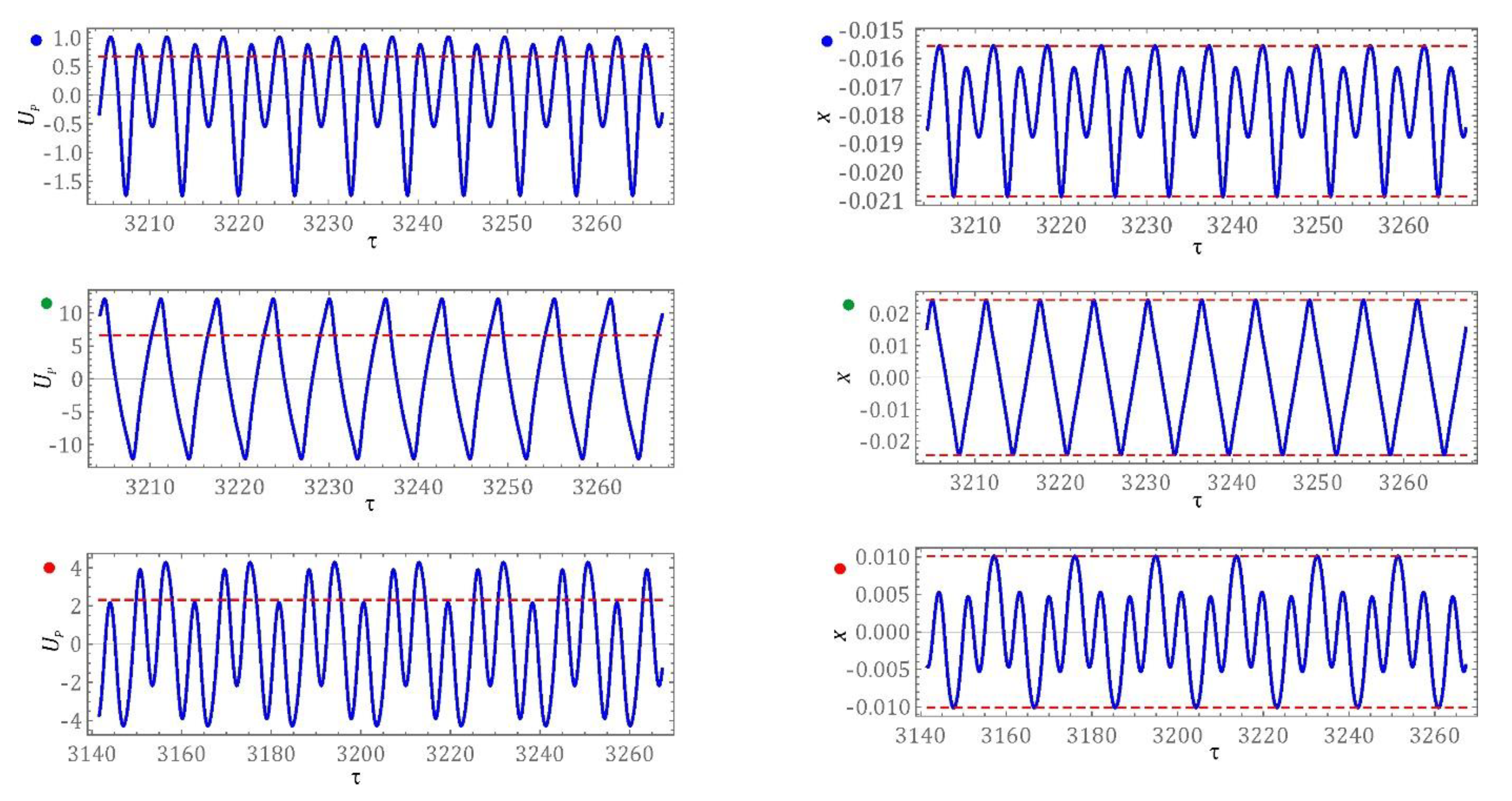
In Figure 6, for better clarity, we also show the corresponding time series of the voltage output and tip mas displacement plotted for small, medium and large power outputs (note that subfigures of Figure 6 correspond the blue, red, and green points in in Figure 5). One can see that the case with fairly large power output corresponds the large amplitude displacement variation signalling the inter well oscillations while the small and medium power output indicates oscillations localized to single potential wells.

5. Conclusions

Based on the conducted model research, it is possible to draw the important conclusions which could be used in future design. It was found that energy harvesting is most effective for one of multiple solutions for which the beam vibration amplitude takes the highest value. For this reason, knowledge of the initial conditions is very important. They can be determined on the basis of basins of attraction.

To effectively harvest energy in the TEH system under analysis, the beam vibration energy level must be large enough for the phase trajectory to pass through the potential barriers. On the other hand, if the beam vibration energy level is too low, then the phase trajectory is limited by potential barriers. Consequently, the higher energy of mechanical inter well vibrations acting on the piezoelectric transducer induces fairly large enough voltage output.

Based on the diagram of the RMS value of the voltage output on the piezoelectric electrodes (Figure 2b), it is possible to estimate the energy that can be harvested from mechanical vibrations.

By changing the excitation frequency various multiple solutions appear. Some of them are characterized by a large orbit with a dominant frequency of excitation, sub- and super-harmonics, and chaotic solutions.

Bearing in mind the effective energy harvesting from vibrating mechanical systems it is required to design the structure so that it is possible to set initial conditions. Without proper calibration of the initial conditions, the effectiveness is significantly reduced. Note that in the system additionally disturbed by stochastic forces larger relative sizes of particular basins of attraction could stabilize solutions [50].

The studied structure is characterized by a frequency broad band and have a great potential to apply in ambient vibration energy. Note that energy harvesting is most effective if the frequency of external excitation ω > 0.5. In the model tests carried out, the highest RMS values of the voltage output (U_RMS > 5V) induced on the piezoelectric electrodes were recorded in relation to the inter-well solutions. All these solutions are characterized by the periodicity of 1T. To get large orbit sub-harmonic solutions as reported in double well potentials [18,19,20] one needs, presumably, to adjust the parameters of the potential wells including their shapes and depths and variate the amplitude of excitation [51].