
Workflow for Probabilistic Resource Estimation: Jafurah Basin Case Study (Saudi Arabia)


Abstract
:1. Introduction
2. Study Region Characteristics
2.1. Petroleum System
2.2. Thermal Maturity
2.3. Sorbed Gas
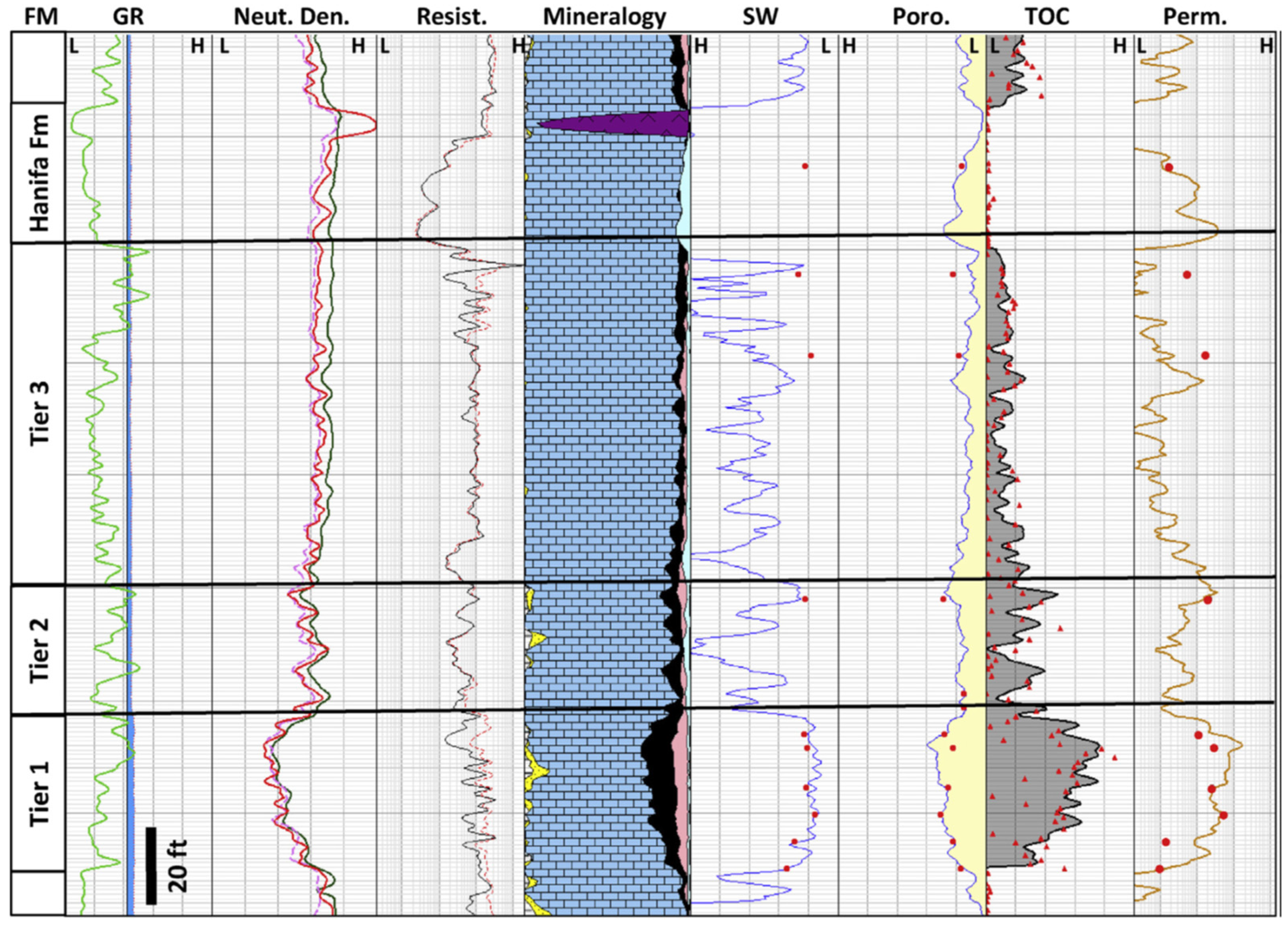
2.4. Target Zones
2.5. TWQ and Eagle Ford Shale Analog
2.6. Natural Fractures and Permeability
2.7. Tectonic Closure Pressure and Fluid Overpressure
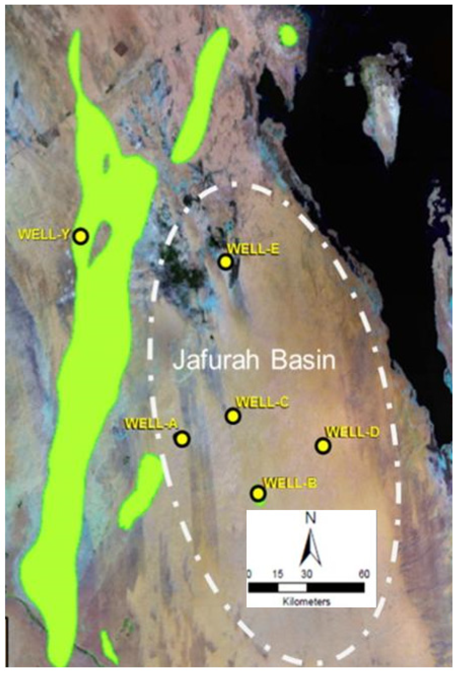
2.8. Exploration Wells
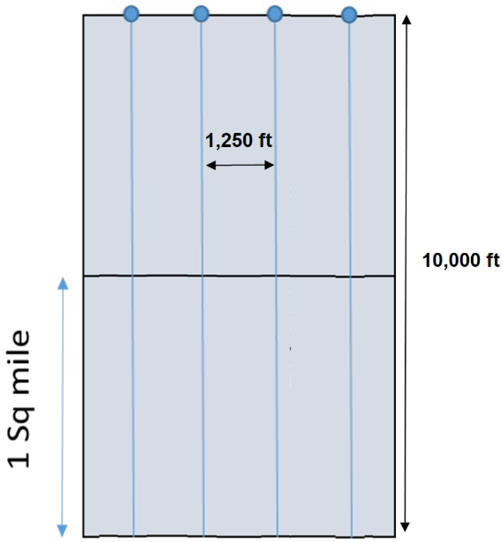
2.9. Drilling Program
2.10. Completions
3. Method of Solution and Data Inputs
3.1. Volumetric Equations
3.2. Deterministic Inputs
3.3. Probabilistic Inputs: Thickness and Distributions
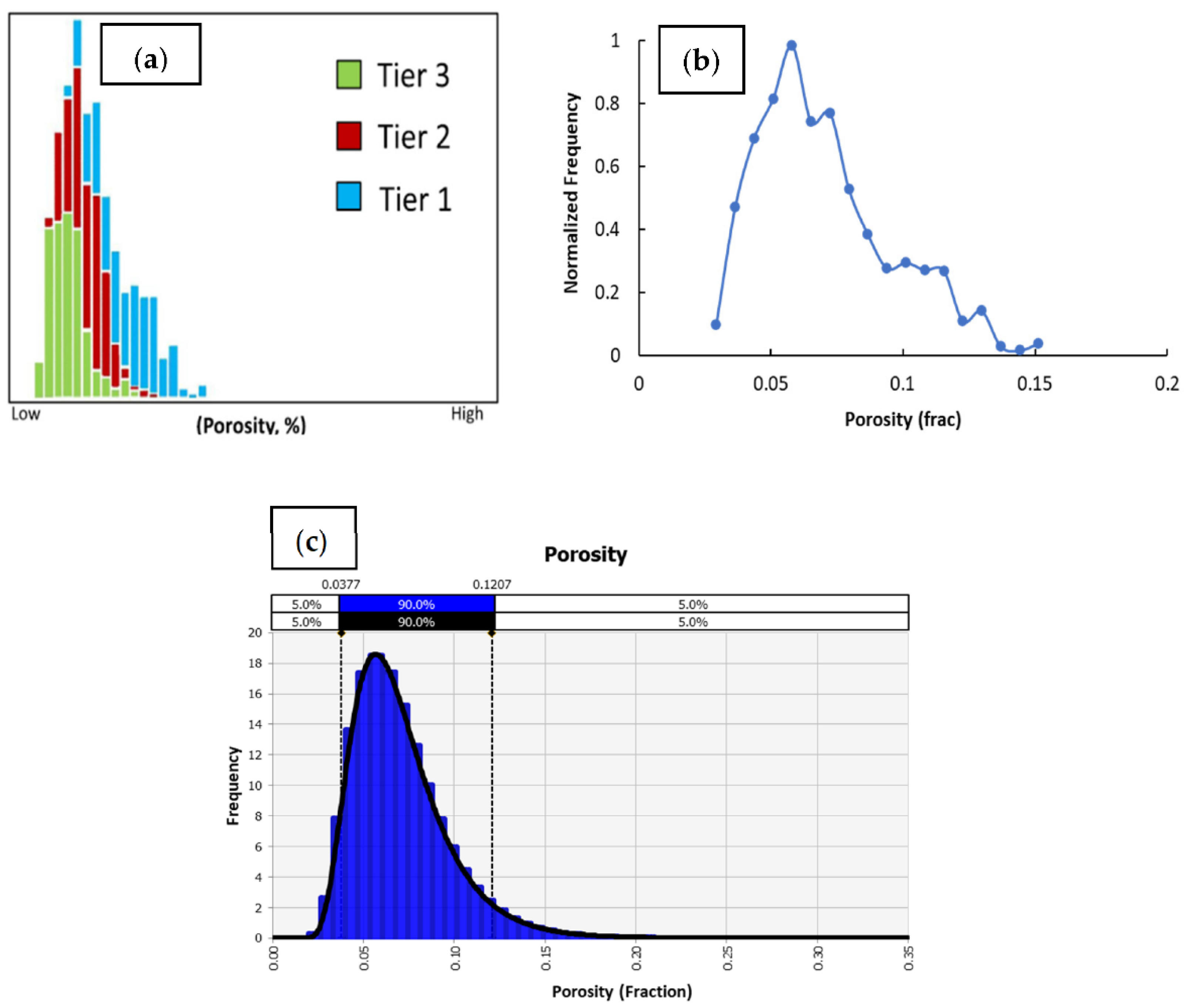
3.4. Porosity
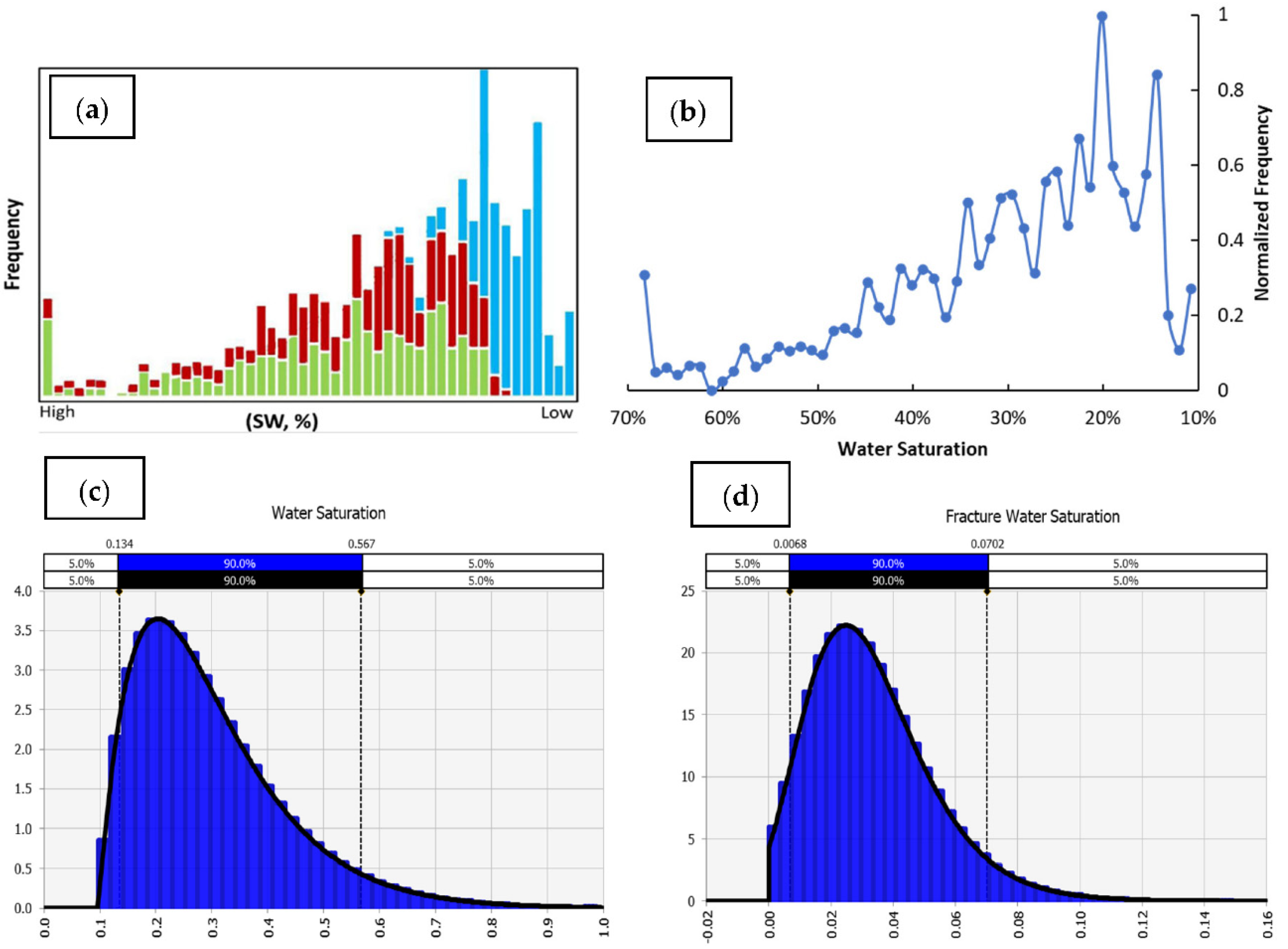
3.5. Formation Water Saturation
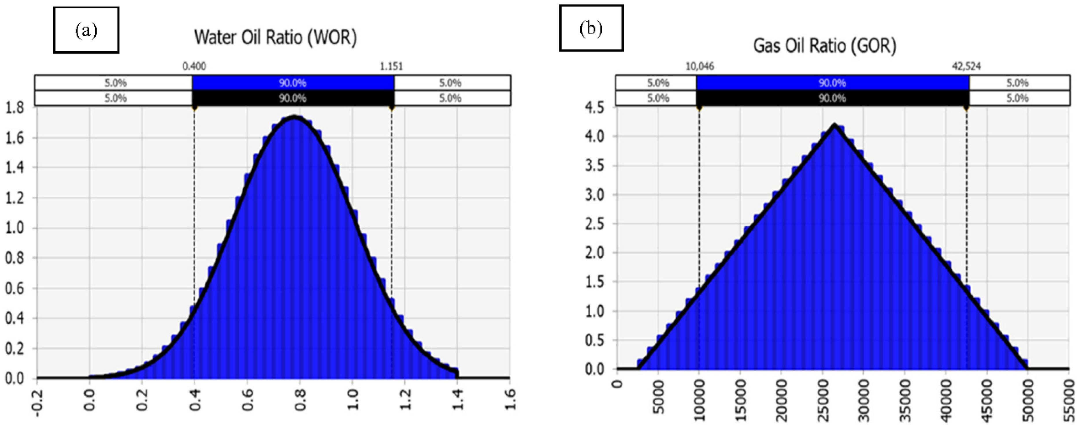
3.6. Water–Oil Ratio (WOR) and Gas–Oil Ratio (GOR)
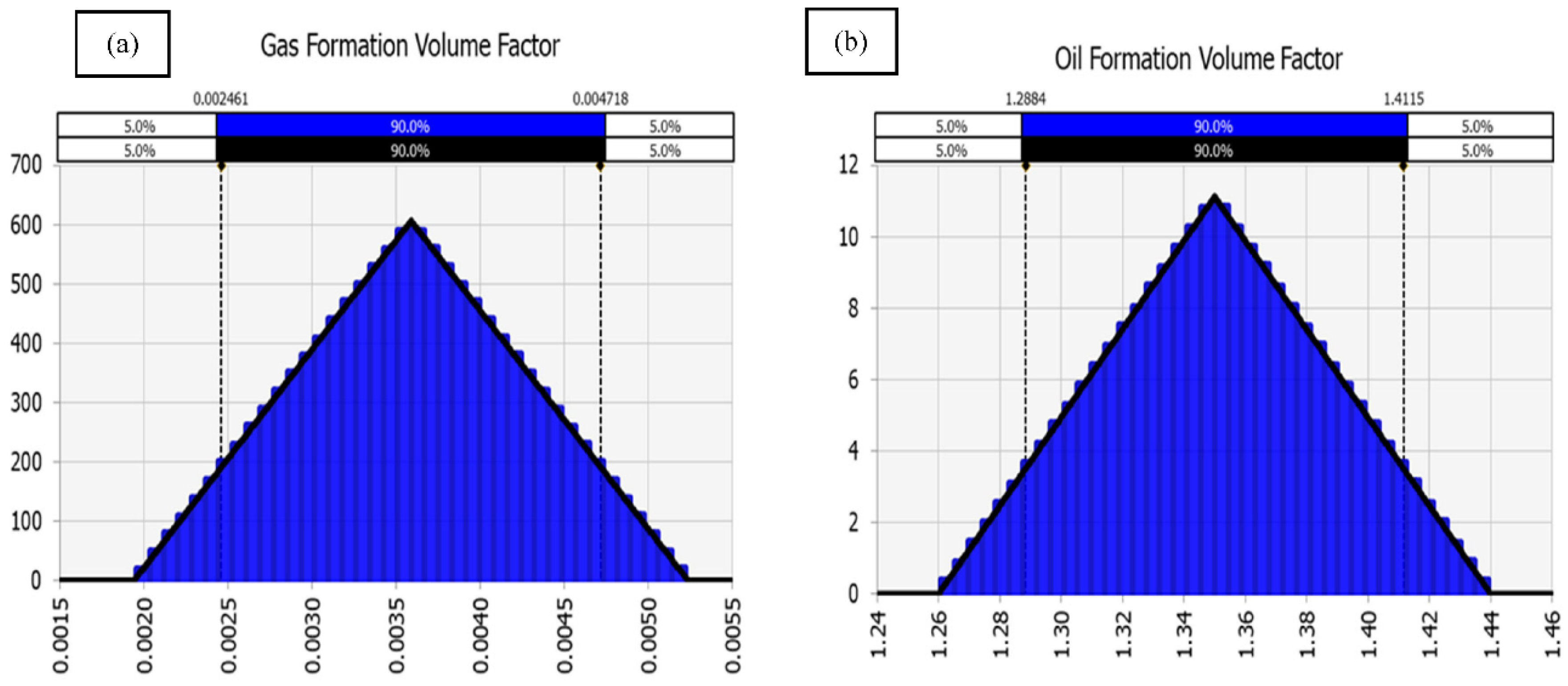
3.7. Gas and Oil Formation Volume Factors
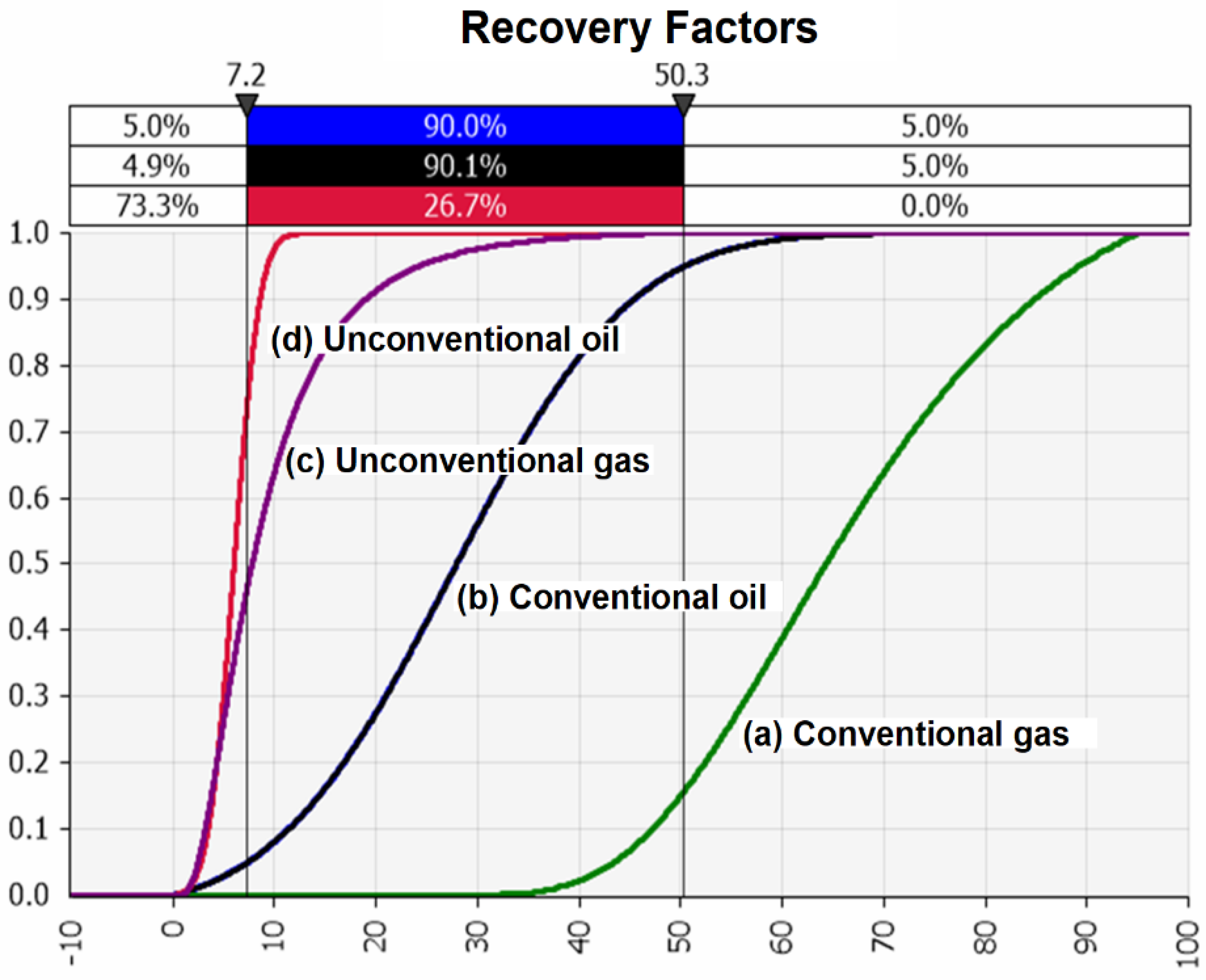
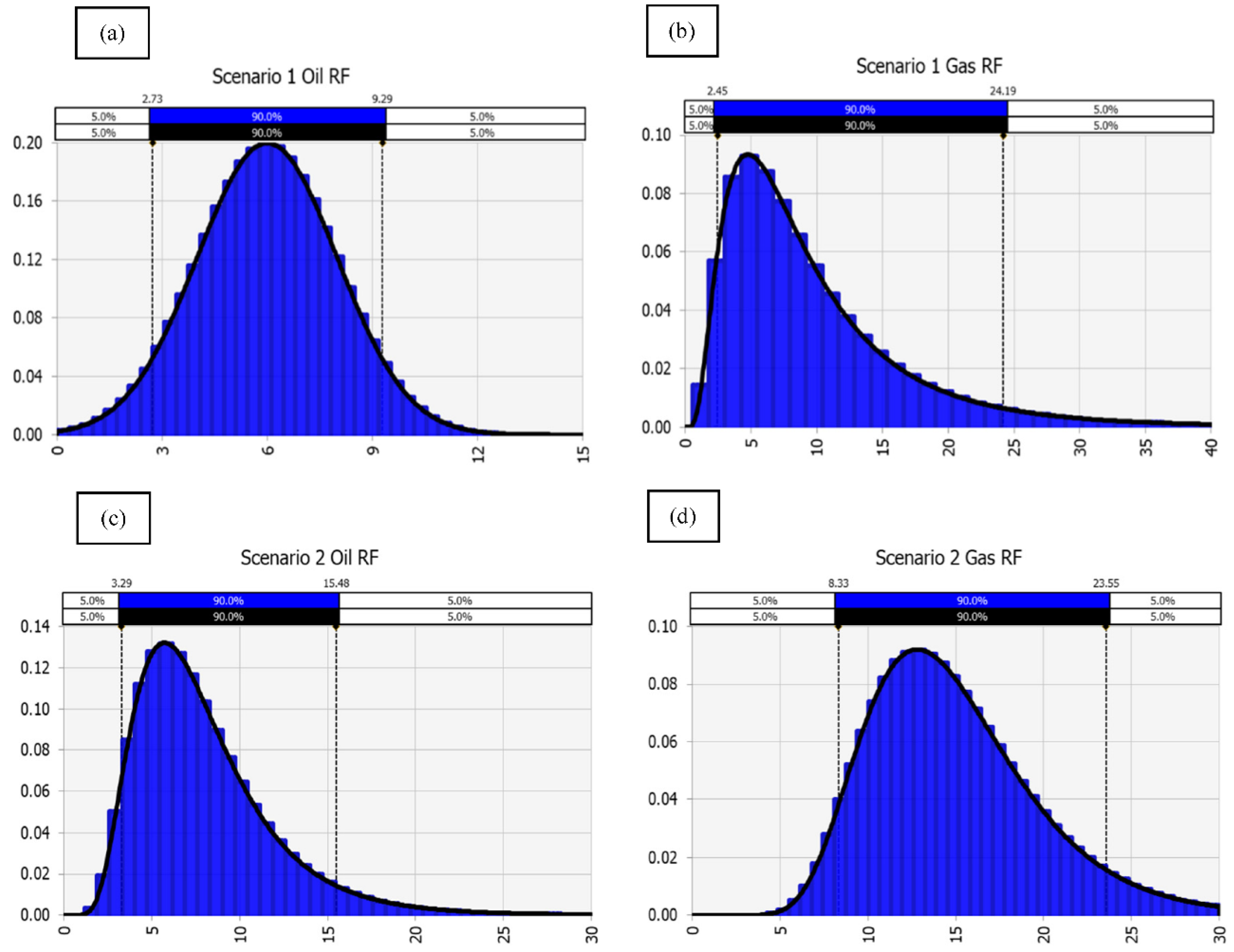
3.8. Recovery Factor
4. Results
4.1. Deterministic EUR Estimations
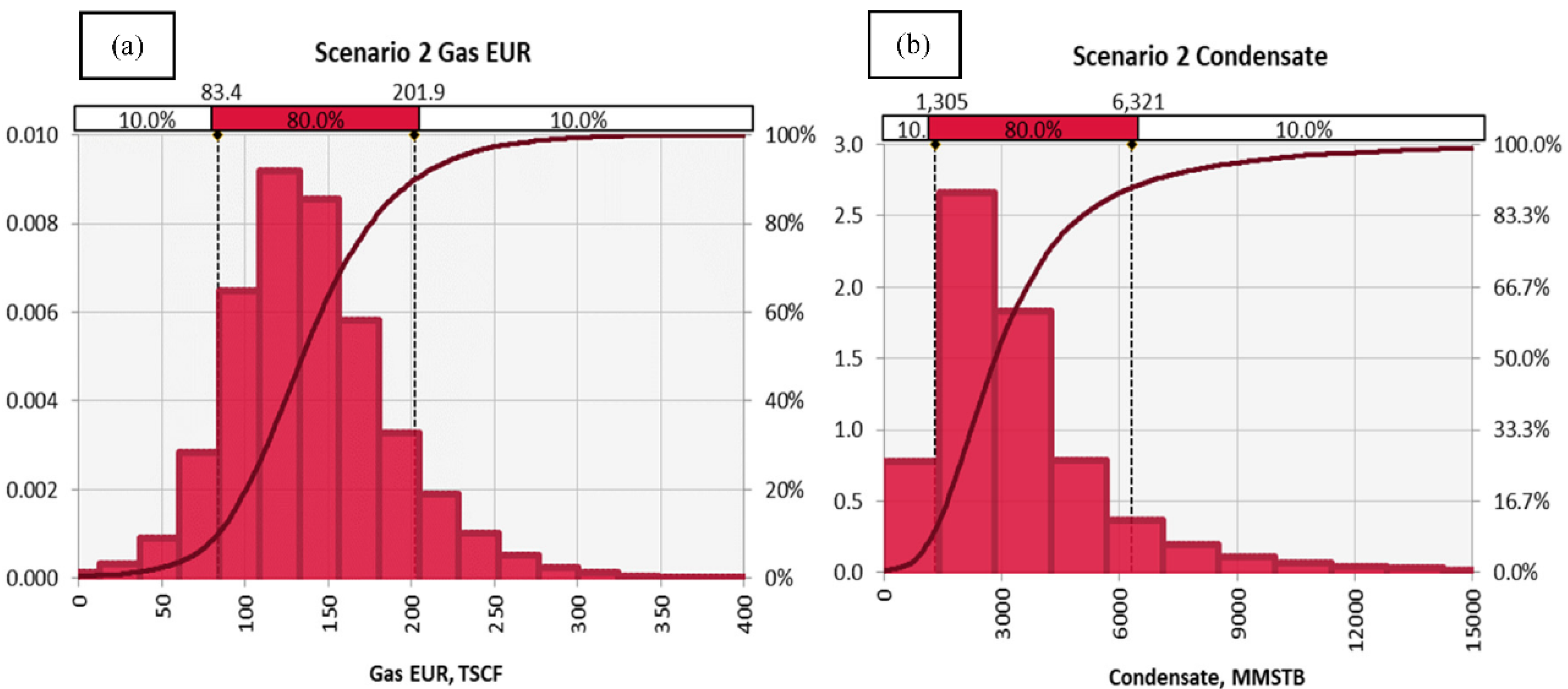
4.2. Probabilistic EUR Estimations
5. Discussion
5.1. Probabilistic Aggregation Effects
5.2. Comparison of Various Resources Estimations
5.3. Limitations
6. Conclusions
Author Contributions
Funding
Acknowledgments
Conflicts of Interest
Nomenclature
| Field area, acres | |
| Gas formation volume factor, rcf/scf | |
| Oil formation volume factor, rbbl/stb | |
| 1359, a constant based on equation units | |
| 43,560, a constant based on equation units | |
| Gas estimated ultimate recovery, scf | |
| Condensate estimated ultimate recovery, stb | |
| Gas content, scf/ton | |
| Gas–oil ratio, scf/stb | |
| Formation height, ft. | |
| Original condensate in place, stb | |
| Free gas in place, scf | |
| Sorbed gas in place, scf | |
| Original gas in place, scf | |
| Pressure, psi | |
| Langmuir pressure, psi | |
| Gas recovery factor, % | |
| Oil recovery factor, % | |
| Fracture water saturation | |
| Matrix water saturation | |
| Langmuir volume scf/ton | |
| Water–oil ratio, stb/stb | |
| Fracture porosity | |
| Matrix porosity | |
| Rock density, g/cc |
Appendix A. Definition of Reserves
References
- BP. BP Statistical Review of World Energy 67th Edition. 2018. Available online: https://www.bp.com/content/dam/bp/business-sites/en/global/corporate/pdfs/energy-economics/statistical-review/bp-stats-review-2018-full-report.pdf (accessed on 28 November 2021).
- Shabaneh, R.; Schenckery, M. Assessing energy policy instruments: LNG imports into Saudi Arabia. Energy Policy 2019, 137, 1–28. [Google Scholar] [CrossRef]
- Mills, R. Under a Cloud: The Future of Middle East Gas Demand. 2020. Available online: www.energypolicy.columbia.edu/MiddleEastGas_CGEP-Report_042920 (accessed on 28 November 2021).
- Shabaneh, R.; Rioux, B.; Griffiths, S. Can Cooperation Enhance Natural Gas Utilization in the GCC? 2020. Available online: https://www.kapsarc.org/research/publications/can-cooperation-enhance-natural-gas-utilization-in-the-gcc/ (accessed on 28 November 2021).
- Talipova, A.; Parsegov, S. Evolution of natural gas business model with deregulation, financial instruments, technology solutions, and rising LNG export. Comparative study of projects inside the US and abroad. In Proceedings of the SPE Annual Technical Conference and Exhibition, Dallas, TX, USA, 24–26 September 2018. [Google Scholar] [CrossRef]
- Shabaneh, R.; Suwailem, M.A. The Prospect of Unconventional Gas Development in Saudi Arabia. 2020. Available online: https://www.kapsarc.org/research/publications/the-prospect-of-unconventional-gas-development-in-saudi-arabia/ (accessed on 28 November 2021).
- Elass. Saudi Aramco Looks to Expand Shale Gas Production. 2018. Available online: https://thearabweekly.com/saudi-aramco-looks-expand-shale-gas-production (accessed on 28 November 2021).
- Aldubyan, M.; Gasim, A. Energy price reform in Saudi Arabia: Modeling the economic and environmental impacts and understanding the demand response. Energy Policy 2021, 148, 111941. [Google Scholar] [CrossRef]
- Weijermars, R.; Moeller, J. Saudi Aramco Privatization in Perspective: Financial Analysis and Future Implications. J. Financ. Econ. 2020, 8, 161–170. [Google Scholar] [CrossRef]
- Weijermars, R. Weighted Average Cost of Retail Gas (WACORG) highlights pricing effects in the US gas value chain: Do we need wellhead price-floor regulation to bail out the unconventional gas industry? Energy Policy 2016, 1139, 6291–6300. [Google Scholar] [CrossRef]
- Kurison, C.; Kuleli, H.S.; Al-Mubarak, A.H. Early and reliable estimation of shale deliverability and spatial drainage parameters from stimulated exploration vertical wells: Case study on Eagle Ford. J. Nat. Gas Sci. Eng. 2020, 84, 103501. [Google Scholar] [CrossRef]
- Hakami, A.M. Characterization of the Carbonate Mud Rocks of the Middle Jurassic Tuwaiq Mountain Formation, Jafurah Sub-basin, Saudi Arabia; Implication for Unconventional Reservoir Quality Prediction. Ph.D. Thesis, King Fahd University of Petroleum and Minerals, Dhahran, Saudi Arabia, December 2016. [Google Scholar]
- Weijermars, R.; Al-Shehri, D. Regulation of Oil and Gas Reserves Reporting in Saudi Arabia: Review and Recommendations. J. Pet. Sci. Eng. 2021, 2021, 109806. [Google Scholar] [CrossRef]
- WoodMackenzie. Jafurah Basin Unconventional Gas. 2020. Available online: https://www.woodmac.com/reports/upstream-oil-and-gas-jafurah-basin-unconventional-gas-70631314/ (accessed on 28 November 2021).
- SPE. Petroleum Reserves Definition. 1997. Available online: https://www.spe.org/en/industry/petroleum-reserves-definitions/ (accessed on 28 November 2021).
- SPE; WPC; AAPG; SPEE; SEG; SPWLA; EAGE. Petroleum Resources Management System. 2018, p. 208. Available online: https://netherlandsewell.com/wpcontent/uploads/2018/09/SPE_Petroleum_Resources_Management_System_2018.pdf (accessed on 28 November 2021).
- Hakami, A.; Al-Mubarak, A.; Al-Ramadan, K.; Kurison, C.; Leyva, I. Characterization of carbonate mudrocks of the Jurassic Tuwaiq Mountain Formation, Jafurah basin, Saudi Arabia: Implications for unconventional reservoir potential evaluation. J. Nat. Gas Sci. Eng. 2016, 33, 1149–1168. [Google Scholar] [CrossRef]
- Hakami, A.; Ellis, L.; Al-Ramadan, K.; Abdelbagi, S. Mud gas isotope logging application for sweet spot identification in an unconventional shale gas play: A case study from Jurassic carbonate source rocks in Jafurah Basin, Saudi Arabia. Mar. Pet. Geol. 2016, 76, 133–147. [Google Scholar] [CrossRef]
- Al Ansari, Y.; Fateh, A.; Shehab, A.; Almoulani, G.; Ghosh, A.; Ahmed, A.; Thampi, S. Hanifa-Tuwaiq Mountain Zone: The edge between conventional and unconventional systems? In Proceedings of the 12th Middle East Geosciences Conference and Exhibition, Manama, Bahrain, 7–10 June 2016; pp. 1–14. [Google Scholar]
- Cantrell, D.L.; Nicholson, P.G.; Hughes, G.W.; Miller, M.A.; Buhllar, A.G.; Abdelbagi, S.T.; Norton, A.K. Tethyan petroleum systems of Saudi Arabia. AAPG Mem. 2014, 106, 613–639. [Google Scholar] [CrossRef]
- Hakami, A.; İnan, S. A basin modeling study of the Jafurah Sub-Basin, Saudi Arabia: Implications for unconventional hydrocarbon potential of the Jurassic Tuwaiq Mountain Formation. Int. J. Coal Geol. 2016, 165, 201–222. [Google Scholar] [CrossRef]
- Weijermars, R. Plio-Quaternary Movement of the East Arabian Block. GeoArabia 1998, 3, 509–540. [Google Scholar] [CrossRef]
- Pepper, A.S.; Corvi, P.J. Simple kinetic models of petroleum formation. Part III: Modelling an open system. Mar. Pet. Geol. 1995, 12, 417–452. [Google Scholar] [CrossRef]
- Montgomery, S.L.; Jarvie, D.M.; Bowker, K.A.; Pollastro, R.M. Mississippian Barnett Shale, Forth Worth basin, north-central Texas: Gas-shale play with multi-trillion cubic foot potential. AAPG Bull. 2005, 89, 155–175. [Google Scholar] [CrossRef]
- Heller, R.; Zoback, M. Adsorption of methane and carbon dioxide on gas shale and pure mineral samples. J. Unconv. Oil Gas Resour. 2014, 8, 14–24. [Google Scholar] [CrossRef] [Green Version]
- Gasparik, M.; Bertier, P.; Gensterblum, Y.; Ghanizadeh, A.; Krooss, B.M.; Littke, R. Geological controls on the methane storage capacity in organic-rich shales. Int. J. Coal Geol. 2014, 123, 34–51. [Google Scholar] [CrossRef]
- Almubarak, A.; Hakami, A.; Leyva, I.; Kurison, C. Saudi Arabia’s unconventional program in the Jafurah basin: Transforming an idea to reality with the Jurassic Tuwaiq mountain formation. In Proceedings of the 22nd World Petroleum Congress, Istanbul, Turkey, 9–13 July 2017. [Google Scholar]
- Al-Momin, A.; Mechkak, K.; Bartko, K.; McClelland, K.; Tineo, R.; Drouillard, M.; Muhammad, N. Cluster Spacing Optimization through Data Integration Workflow for Unconventional Jurassic Mudrocks, Saudi Arabia, SPE184830. Presented at the SPE Hydraulic Fracturing Technology Conference and Exhibition, The Woodlands, TX, USA, 24–26 January 2017. [Google Scholar] [CrossRef]
- Ba Geri, M.; Ellafi, A.; Flori, R.; Belhaij, A.; Ethar, H.A. New Opportunities and Challenges to Discover and Develop Unconventional Plays in the Middle East and North Africa: Critical Review, SPE197271. Presented at the Abu Dhabi International Petroleum Exhibition & Conference, Abu Dhabi, United Arab Emirates, 11–14 November 2019. [Google Scholar] [CrossRef]
- Kurison, C.; Kuleli, H.S.; Mubarak, A.H. Unlocking well productivity drivers in Eagle Ford and Utica unconventional resources through data analytics. J. Nat. Gas Sci. Eng. 2019, 71, 102976. [Google Scholar] [CrossRef]
- Gala, D.; Sharma, M. Compositional and geomechanical effects in Huff-n-Puff gas injection ior in tight oil reservoirs. In Proceedings of the SPE Annual Technical Conference and Exhibition, Dallas, TX, USA, 24–26 September 2018. [Google Scholar] [CrossRef]
- Al-Momin, A.; Kurdi, M.; Baki, S.; Mechkak, K.; Al-Saihati, A. Proving the concept of unconventional gas reservoirs in Saudi through multistage fractured horizontal wells. In Proceedings of the SPE Asia Pacific Unconventional Resource Conference and Exhibition, Brisbane, Australia, 9–11 November 2015. [Google Scholar] [CrossRef]
- Weijermars, R.; Nandlal, K.; Khanal, A.; Tugan, M.F. Comparison of Pressure Front with Tracer Front Advance and Principal Flow Regimes in Hydraulically Fractured Wells in Unconventional Reservoirs. J. Pet. Sci. Eng. 2019, 183, 106407. [Google Scholar] [CrossRef]
- Weijermars, R. Improving Well Productivity—Ways to Reduce the Lag between the Diffusive and Convective Time of Flight in Shale Wells. J. Pet. Sci. Eng. 2020, 193, 107344. [Google Scholar] [CrossRef]
- Al-Mulhim, N.I.; Korosa, M.; Ahmed, A.; Hakami, A.; Sadykov, A.; Baki, S.; Asiri, K.S.; Al Ruwaished, A. Saudi Arabia’s Emerging Unconventional Carbonate Shale Resources: Moving to Horizontals with an Integrated Engineering and Geosciences Approach, SPE 176936. Presented at the SPE Asia Pacific Unconventional Resources Conference and Exhibition, Brisbane, Austria, 9–11 November 2015. [Google Scholar]
- Kurison, C.; Kuleli, H.S.; Mubarak, A.H.; Al-Sultan, A.; Shehri, S.J. Reducing uncertainty in unconventional reservoir hydraulic fracture modeling: A case study in Saudi Arabia. J. Nat. Gas Sci. Eng. 2019, 71, 102948. [Google Scholar] [CrossRef]
- Weijermars, R.; van Harmelen, A.; Zuo, L.; Nascentes Alves, I.; Yu, W. Flow interference between hydraulic fractures. SPE Reserv. Eval. Eng. 2018, 21, 942–960. [Google Scholar] [CrossRef]
- Energent. Overview of Wells Drilled in US Shale Basin on an Annual Basis. 2021. Available online: https://www.westwoodenergy.com/business-division/research/world-land-drilling-rig-market-forecast-2021-2025 (accessed on 28 November 2021).
- EIA. Permian Basin: Wolfcamp Shale Play Geology Review, Independent Statistics & Analysis; U.S. Energy Information Administration: Washington, DC, USA, 2018. [Google Scholar]
- EIA. The Distribution of U.S. Oil and Natural Gas Wells by Production Rate; U.S. Energy Information Administration: Washington, DC, USA, 2020. Available online: https://www.eia.gov/petroleum/wells/pdf/full_report.pdf (accessed on 28 November 2021).
- Al-Mulhim, N.; Saihati, A.; Hakami, A.; Al Harbi, M.; Asiri, K. First successful proppant fracture for unconventional carbonate source rock in Saudi Arabia. In Proceedings of the International Petroleum Technology Conference, Kuala Lumpur, Malaysia, 10–12 December 2014; pp. 581–593. [Google Scholar] [CrossRef]
- Al-Sulami, G.; Boudjatit, M.; Al-Duhailan, M.; Salvatore, D.S. The Unconventional Shale Reservoirs of Jafurah Basin: An Integrated Petrophysical Evaluation Using Cores and Advanced Well Logs. SPE 183771. Presented at the SPE Middle East Oil & Gas Show and Conference, Manama, Bahrain, 6–9 March 2017; Available online: https://doi.org/10.2118/183771-MS (accessed on 28 November 2021).
- Aguilera, R. Shale gas reservoirs: Theoretical, practical and research issues. Pet. Res. 2016, 1, 10–26. [Google Scholar] [CrossRef]
- Dong, Z. A New Global Unconventional Natural Gas Resource Assessment. Ph.D. Thesis, Texas A&M University, College Station, TX, USA, August 2012. [Google Scholar]
- Dong, Z.; Holditch, S.A.; McVay, D.A.; Ayers, W.B.; Lee, W.J.; Morales, E. Probabilistic assessment of world recoverable shale gas resources. In Proceedings of the European Unconventional Resources Conference and Exhibition, Vienna, Austria, 25–27 February 2014. [Google Scholar] [CrossRef]
- EIA. shale gas and shale oil resource assessment methodology. In EIA/ARI World Shale Gas and Shale Oil Resource Assessment; U.S. Energy Information Administration: Washington, DC, USA, 2013; pp. 1–23. [Google Scholar]
- Richardson, J.; Yu, W.; Weijermars, R. Benchmarking recovery factors of individual wells using a probabilistic model of original gas in place to pinpoint the good, bad and ugly producers. In Proceedings of the SPE/AAPG/SEG Unconventional Resources Technology Conference, San Antonio, TX, USA, 1–3 August 2016. [Google Scholar] [CrossRef]
- Richardson, J.; Yu, W. Calculation of estimated ultimate recovery and recovery factors of shale-gas wells using a probabilistic model of original gas in place. SPE Reserv. Eval. Eng. 2018, 21, 638–653. [Google Scholar] [CrossRef]
- Yu, W.; Sepehrnoori, K.; Patzek, T.W. Modeling gas adsorption in Marcellus shale with langmuir and bet isotherms. SPE J. 2016, 21, 589–600. [Google Scholar] [CrossRef] [Green Version]
- Hammes, U.; Eastwood, R.; McDaid, G.; Vankov, E.; Gherabati, S.A.; Smye, K.; Tinker, S. Regional assessment of the Eagle Ford group of South Texas, USA: Insights From lithology, pore volume, water saturation, organic richness, and productivity correlations. Interpretation 2016, 4, 1F–T121. [Google Scholar] [CrossRef]
- Laherrere, J. Oil and Gas: What Future ? In Groningen Annual Energy Convention; 2006. Available online: http://aspofrance.viabloga.com/files/JL-Groningen-long.pdf (accessed on 28 November 2021).


| 500 | 1000 | 2000 | |
|---|---|---|---|
| C1 | 31.231 | 44.522 | 56.447 |
| N2 | 0.073 | 0.104 | 0.132 |
| C2 | 4.314 | 5.882 | 7.288 |
| C3 | 4.148 | 4.506 | 4.827 |
| CO2 | 1.282 | 1.821 | 2.306 |
| iC4 | 1.35 | 1.298 | 1.251 |
| nC4 | 3.382 | 2.978 | 2.615 |
| iC5 | 1.805 | 1.507 | 1.24 |
| nC5 | 2.141 | 1.711 | 1.325 |
| nC6 | 4.623 | 3.28 | 2.076 |
| C7+ | 16.297 | 11.563 | 7.316 |
| C11+ | 12.004 | 8.94 | 5.924 |
| C15+ | 10.044 | 7.127 | 4.509 |
| C20+ | 7.306 | 4.762 | 2.745 |
| Data Source | Name, Unit | Min Value | Max Value |
|---|---|---|---|
| TWQ MN Public (1) | Formation height, ft | 110 | 150 |
| TWQ MN Public (1) | Matrix porosity | 0.05 | 0.12 |
| Typical parameter | Fracture porosity | 0.01 | 0.03 |
| TWQ MN Public (1) | Formation pressure, psi | 4550 | |
| TWQ MN Public (1) | GCR or GOR, scf/stb | 2500 | 50,000 |
| Aguilera, 2016 (2) | GCR, scf/stb | 2700 | 48,300 |
| Eagle Ford Analogue (3) | WOR | 1 | |
| Aguilera, 2016 (2) | Gas formation volume factor, rcf/scf | 0.00194 | 0.00524 |
| Eagle Ford Analogue (3) | Oil formation volume factor, rbbl/stb | 1.3 | 1.4 |
| Marcellus (4) | Langmuir volume, scf/ton | 100 | 200 |
| Marcellus (4) | Langmuir pressure, psi | 500 | 1000 |
| Eagle Ford Analogue (3) | Oil recovery factor, % | 1 | 10 |
| Eagle Ford Analogue (3) | Gas recovery factor, % | 10 | 20 |
| General Value | Rock density, g/cc | 2.3 | 2.8 |
| Hammes, 2016 (5) | Matrix water saturation | 0.1 | 0.4 |
| Hammes, 2016 (5) | Fracture water saturation | 0 | 0.4 |
| Parameter | Distribution |
|---|---|
| Thickness | Uniform |
| Porosity | Log Normal |
| Gas–oil ratio (GOR) | Triangular |
| Gas formation volume factor (Bg) | Triangular |
| Oil formation volume factor (Bo) | Triangular |
| Oil recovery factor | Normal |
| Gas recovery factor | Log Normal |
| Formation water saturation | Gamma |
| Fracture saturation | Log Normal |
| Water–oil ratio (WOR) | Normal |
| Parameter | Min | Most Likely | Max |
|---|---|---|---|
| GOR (scf/stb) | 2500 | 26,500 | 50,000 |
| Bg | 1.29 × 10⁻³ | 3.59 × 10⁻³ | 5.24 × 10⁻³ |
| Bo | 1.26 | 1.35 | 1.44 |
| Estimation | Minimum | Expected (Mean) | Maximum |
|---|---|---|---|
| Uncertainty | Most conservative | Most likely | Most optimistic |
| Formation height, ft | 110 | 130 | 150 |
| Matrix porosity | 0.05 | 0.085 | 0.12 |
| Fracture porosity | 0.01 | 0.02 | 0.03 |
| Formation pressure, psi | 4550 | 4550 | 4550 |
| GCR or GOR, scf/stb | 50,000 | 26,250 | 2500 |
| GCR, scf/stb | 48,300 | 25,500 | 2700 |
| WOR | 1 | 1 | 1 |
| Gas formation volume factor, rcf/scf | 0.00524 | 0.00359 | 0.00194 |
| Oil formation volume factor, rbbl/stb | 1.4 | 1.35 | 1.3 |
| Langmuir volume, scf/ton | 100 | 150 | 200 |
| Langmuir pressure, psi | 1000 | 750 | 500 |
| Oil recovery factor, % | 1 | 5.5 | 10 |
| Gas recovery factor, % | 10 | 15 | 20 |
| Rock density, g/cc | 2.3 | 2.55 | 2.8 |
| Matrix water saturation | 0.4 | 0.25 | 0.1 |
| Fracture water saturation | 0.4 | 0.2 | 0 |
| Estimation | Minimum (P90) | Expected (Mean; P50) | Maximum (P10) |
|---|---|---|---|
| , scf/ton | 81.98 | 128.77 | 180.20 |
| , Tscf | 7.24 | 237.54 | 1359.55 |
| , Tscf | 87.38 | 171.23 | 288.32 |
| , Tscf | 94.62 | 408.77 | 1647.87 |
| , Tscf | 9.46 | 61.32 | 329.57 |
| , Bstb | 1.89 | 15.57 | 659.15 |
| , MMstb | 18.92 | 856.47 | 65,914.68 |
| Parameter | Distribution | Mean | Standard Deviation | |
|---|---|---|---|---|
| Scenario 1 | Gas RF | Log normal | 6 | 2 |
| Oil RF | Normal | 10 | 8 | |
| Scenario 2 | Gas RF | Log normal | 15 | 4 |
| Oil RF | Normal | 27 | 6.5 |
| Parameter | Case | P90 | P50 | P10 | Mean | Standard Deviation |
|---|---|---|---|---|---|---|
| Gas EUR, TSCF | Scenario 1 | 14 | 37 | 99 | 49 | 41 |
| Scenario 2 | 83 | 134 | 202 | 134 | 51 | |
| Condensate, MMSTB | Scenario 1 | 474 | 1118 | 2599 | 1411 | 1174 |
| Scenario 2 | 1305 | 2840 | 6321 | 3533 | 2883 |
| Average EUR (bcfe) | |||||
|---|---|---|---|---|---|
| Number of Wells | 1 | 10 | 100 | 1000 | 10,000 |
| Mean | 2.1 | 20.9 | 209.4 | 2094.5 | 20,944 |
| P10 | 3.1 | 24.2 | 220.0 | 2126.7 | 21,043 |
| P50 | 2.0 | 20.8 | 209.2 | 2094.9 | 20,943 |
| P90 | 1.1 | 17.7 | 199.2 | 2061.9 | 20,845 |
| P50 EURs | Natural Gas (TCF) | Condensate and NGLs (Billion BBls) | Total Gas Equivalent (Tcfe) |
|---|---|---|---|
| Deterministic (Section 4.1) | 61.32 | 0.856 | 66.6 |
| Probabilistic Scenario 1 (Section 4.2) | 37.00 | 1.118 | 43.7 |
| Probabilistic Scenario 2 (Section 4.2) | 134.00 | 2.840 | 151.2 |
| Deterministic WoodMackenzie [14] | 17.18 | 8.264 | 67.4 |
Publisher’s Note: MDPI stays neutral with regard to jurisdictional claims in published maps and institutional affiliations. |
© 2021 by the authors. Licensee MDPI, Basel, Switzerland. This article is an open access article distributed under the terms and conditions of the Creative Commons Attribution (CC BY) license (https://creativecommons.org/licenses/by/4.0/).
Share and Cite
Weijermars, R.; Jin, M.; Khamidy, N.I. Workflow for Probabilistic Resource Estimation: Jafurah Basin Case Study (Saudi Arabia). Energies 2021, 14, 8036. https://doi.org/10.3390/en14238036
Weijermars R, Jin M, Khamidy NI. Workflow for Probabilistic Resource Estimation: Jafurah Basin Case Study (Saudi Arabia). Energies. 2021; 14(23):8036. https://doi.org/10.3390/en14238036
Chicago/Turabian StyleWeijermars, Ruud, Miao Jin, and Nur Iman Khamidy. 2021. "Workflow for Probabilistic Resource Estimation: Jafurah Basin Case Study (Saudi Arabia)" Energies 14, no. 23: 8036. https://doi.org/10.3390/en14238036
APA StyleWeijermars, R., Jin, M., & Khamidy, N. I. (2021). Workflow for Probabilistic Resource Estimation: Jafurah Basin Case Study (Saudi Arabia). Energies, 14(23), 8036. https://doi.org/10.3390/en14238036