Abstract
Great significance is given to the use of energy from renewable sources, especially in industrial and municipal applications. The present article is devoted to the optimal control of a DFIG generator with the help of a rotor-side converter (RSC). Its aim is to ensure the delivery of the voltage of a three-phase network with appropriate parameters while operating in an islanded grid. Such a grid is usually characterized by an uneven loading of each phase. Additionally, the load of these phases changes randomly in time. In order to ensure the assumed parameters of line voltages, the optimal control is applied with a square cost function. This ensures the shape of voltage that is in accordance with the referential voltage. Moreover, higher harmonics with a given number are detected and reduced. The simulations that were executed confirm compliance with the conditions of the parameters of the output voltage in the islanded grid. Attention was paid to oscillations in the power flowing through the rotor-side converter (RSC). The methods to accelerate the suppression of these oscillations are presented.
1. Introduction
Wind turbines are popular because of their accessibility and the ability to use inexhaustible wind resources. Wind energy can be used by turbines to power a network system. This enables the greater use of renewable sources of energy. There is a wide range of advantages of using a doubly fed induction generator (DFIG) to convert the wind energy powering a wind turbine into electric energy. One of them is the possibility to control the DFIG rotor by the use of a rotor-side converter (RSC). This enables one to influence the network system’s stability, and it allows one to consider wind speed fluctuations while applying various types of wind turbines.
In many cases, an island network is used as a procedure to operate the energy system. This is carried out on the distribution level. This way, it is possible to protect a number of sensitive receivers from the consequences of shutdowns and to ensure the continuity of electricity supply. This procedure can also be applied in the event of network failure. It is necessary to ensure good power quality at the load terminals of the islanded network. A symmetric, independent three-phase voltage system with a neutral conductor is created with a given voltage and angular frequency value. This task is difficult due to the random nature of phase loading. Each phase can be loaded differently. In addition, phase loading may vary randomly over time. In these conditions, the voltage of a separate network should be of a constant, given value in each phase, and the angles between the phases should be of 120 and 240 electric degrees.
Frequently, there are special microgrids created as located groups of generating, storing and load appliances. They should provide self-sufficiency in this part of the network, ensuring function even after the main network is switched off. This may be a crucial option to improve the reliability of a low-voltage network. The limited size of these microgrids has to be taken into account while distributing the energy. At distribution, they may be treated as separate units in the managing procedure, which can be termed ‘islanding’.
Islanding is a division of an electrical grid into fragments that are able to independently meet the demand for power. This should protect sensitive receivers from malfunctions caused by asymmetric three-phase voltages. Islanding can occur as planned; however, it may also appear as a result of turning the line off unexpectedly and uncontrollably. Then, it poses a threat to the applied loads because of the lack of control over voltage and frequency.
This article considers the optimal control of a rotor’s winding of a DFIG generator, which is a part of a wind farm. The control system of the rotor’s voltage is implemented. The method of optimal control with a square cost function was used This cost function provides a reduction in voltage error on a receiver’s terminals. This error is calculated as the difference between this terminal voltage and the reference voltage. At the same time, higher harmonics of the assumed numbers of the three-phase receiver voltage are computed. The cost function ensures a reduction in these higher harmonics, which improves the quality of the voltage on an islanded receiver. The rotor current of the DFIG generator is assumed as the control variable. This makes it possible to control its value, as it should not exceed the nominal rating. The considerations are made in a dq coordinate system rotating with the synchronic speed ω.
The applied method of reducing the higher harmonics of the receiver voltage by their separation and later inclusion in the cost function is a modern solution. As for now, energy hybrid filters ref. [1,2] were used for this aim. Usually, they are a combination of passive filters tuned to given harmonics (e.g., to the seventh harmonic) and active filters. The advantage of using these filters is a reduction in the required converter power. In this solution, the role of the active filter is only to complement the work of the passive filter. It reduces the harmonics that remain after passive filtration. Active filters can be installed in a series or shunt position at the output of the system. The solution described in the present article does not apply passive filters. All the necessary power to reduce the higher harmonics was generated in an RSC system (rotor-side converter). Introduction of passive filters in order to unload the RSC system will be considered in the subsequent paper.
The issue of modeling, control, stability and management of the power of distributed energy sources for islanded micro-networks is also depicted with consideration of the regulation of the amplitude of voltage and frequency in ref. [3]. The suggested method of control for unbalanced and non-linear loads uses a repetitive control scheme to remove the effects of the imbalance and non-linearity of the load. An adaptable compensation in order to increase the stability and robustness of the islanded network in case of network uncertainties is suggested. At the same time, a unified strategy was developed, which enables the operation in an island mode, as well as in grid-connected mode, without the necessity of detecting the current mode of the microgrid.
In the case of extreme failure of the network, the distributing system may be divided into a few energy independent, separate micro-networks ref. [4]. Each of them has to provide a constant power supply. Such a power supply can be provided by the wind farm described in this article. Having isolated the failure, the distribution systems are recovered by connecting micro-networks to the main system. Similar issues are considered in ref. [5]. The controlled islanding of the system depicted there is treated as a last resort to save the system from partial or complete power shut down. For the active detection of islanded micro-networks, the injection of a negative sequence current by a voltage-sourced converter as an interference signal is used in ref. [6]. The proposed control strategy enables a smooth transition between the grid connected and the islanded mode of operation, where the DFIG generators of wind farms can be used.
The importance of providing the appropriate frequency of the islanded grid was pointed out in ref. [7]. In order to ensure high-quality energy in the islanded grid, a strategy of coordinated control between a distributed energy source, such as a DFIG generator of a wind farm, and a battery energy storage system was proposed here. This way, stability of the frequency was provided in the islanded grid. Such a cooperation appears to be advisable so as to improve the quality of the control system of the DFIG generator that is described in this article. However, it was not applied here.
Undoubtedly, higher harmonics of voltage appear to be problematic in an islanded grid. In ref. [8], an innovative method of control is presented for voltage source inverters connected to the grid, which utilizes the droop method. Due to this, inverters are able to provide independently active and reactive power to the grid. The grid characterization technique in this paper ref. [8] is based on processing the voltage on current phasors at the point of common coupling (PCC) between the power converter and the grid. In order to monitor such voltage and current phasors, a frequency-locked loop based on a second-order generalized integrator (SOGI-FLL) is used. In order to reduce the higher harmonics of the islanded grid voltage in this article, the harmonics with given numbers were calculated. They were included in the square cost function, where they were later reduced by the use of the discrete linear quadratic regulator ref. [9].
The issue of connecting distributed generation ref. [4,7] with the distribution network ref. [4] and their cooperation during a failure was presented in ref. [10]. An adaptive control strategy was described in the application in a DFIG generator. The compatibility with a typical feeder automation protection logic in the ring distribution system was also highlighted. The article explains the way in which the DFIG generator cooperated with other generative units, as well as with energy storing units, in order to stabilize the voltage of the islanded network. The description of the use of communication technology through generic object-oriented substation event messages for the DFIG coordination control strategy to cause the DFIG to operate continuously during fault isolation and support islanding is depicted in ref. [11]. In order to connect the DFIG generator of a wind farm located at a distance from the network, a voltage source converter for HVDC transmission system was used in ref. [12]. The working principles of the proposed system were described, and new strategies for operation in average conditions, as well as in the case of network failure, were suggested. During such failures, in order to sustain the voltage, an automatic balancing of the power by modulation of the DFIG generator’s frequency and other parts of wind farm systems is applied. A crucial issue while applying an appropriate control for generators is to detect the occurrence of an islanded grid. The method of detection is based on an adaptive neuro-fuzzy inference system (ANFIS) ref. [13]. It was tested by the use of seven passive monitoring parameters. It introduces a closed-loop algorithm that constantly observes the point of common coupling with a trip signal for a circuit breaker. The inputs of ANFIS training were data acquired by an experimental measurement at the point of common coupling of a real-life photovoltaic power plant system, using automatic meter reading. The project data of the DFIG generator were based on ref. [14]. This paper describes the design and the testing process of the DFIG generator for use in wind turbine applications. Depending on the project requirements, an analytical design is developed, which is then verified using the finite element method.
In Reference [15], the advanced control of a wind power system with a DFIG generator is described. Improved grid integration is achieved due to the use of power electronic converters. An advanced control method of a DFIG generator wind power system under grid fault conditions involving higher harmonic distortions is presented.
In ref. [16], a 10 MW direct-drive DFIG generator for wind turbine operation is designed and optimized analytically. The authors’ consideration of nonlinearities in the magnetic circuit is important. Paper ref. [17] describes the advantages and disadvantages of using a DFIG generator in a wind turbine system. With a DFIG generator, the frequency stabilization of the grid was improved. A large contribution to this was made by the inertial response of the rotor. This improvement is especially important because grids have become more unstable. The reason for this instability is the growth of the distributed power generation, such as wind energy conversion systems. Therefore, technical specification requirements for these decentralized power plants connected to a public grid have increased dramatically. A lower cost for power electronics was also pointed out.
Paper ref. [18] also presents problems related to the decentralization of electricity generation. In dissertation ref. [19], the author describes the physical relationships of wind turbine components. He points out the relationship between the modeling accuracy level and the active and reactive generator output current. The author of ref. [20] describes the difficulties in connecting a DFIG wind turbine system to the grid. He analyzes the dynamic behavior of a DFIG wind turbine system under different types of faults. The problem of wind power fluctuations in the context of connecting a wind farm to the AC grid is also discussed.
Key problems associated with renewable energy, such as the issues of safety, stability, power quality and associated costs, were discussed by the author of paper ref. [21]. Paper ref. [22] highlights a new methodology for the frequency control of micro-grids. The DFIG generator and a battery energy storage system are used in this approach. In ref. [23], a vector control technique without additional simplifications is presented. The MPPT and the pitch control technique are used to control a grid-connected wind energy conversion system with a DFIG generator. On the other hand, in ref. [24], a multi-objective method based on differential evolution is applied for tuning the parameters of rotor- and grid-side converter controllers in a DFIG wind turbine system. Paper ref. [25] presents a control method for a variable-speed wind turbine system with a DFIG generator operating in an islanded grid. Simulation models and the optimal control method of pitch angle and rotating speed as well as fast frequency and voltage regulation during islanding operation are proposed. In paper ref. [26], a multi-mode control strategy for a DFIG generator of a wind power/storage system is proposed. It is shown that the proposed control strategy enables the investigated system to supply the grid with the requested power regardless of the wind conditions. Book ref. [27] discusses various forms of torque control of electrical machines. One type of such control is vector control. The second type of machine torque control discussed in the book is direct torque control. These methods provide a fast torque response, low inverter switching frequency and low harmonic losses. In ref. [28], the authors present an intelligent-based islanding detection algorithm for PV and DFIG units. The decision tree algorithm is used. Paper ref. [29] considers control systems for a stand-alone operation of a DFIG generator. The connection of DFIG to balanced or unbalanced grids and sensorless control are presented. Paper ref. [30] describes the application of a DFIG generator to improve the voltage quality of the grid. The proposed control method helps to maintain the continuous control of the active and reactive power of the DFIG generator under grid disturbances. On the other hand, in ref. [31], the control methods for DFIG generators were reviewed for different aspects of their operation. The possibility of controlling DFIG rotor currents to correct problems caused by unbalanced stator voltages is demonstrated. These are mainly torque pulsations and unbalanced stator currents. It is found that DFIG generators should be disconnected from the grid when the voltage imbalance is greater than 6%. Paper ref. [32] considers the ability of a DFIG generator to regulate grid voltage and its behavior under grid fault conditions. Fifth-order machine models and reduced, third-order models were used. Paper ref. [33] presents the DFIG rotor voltage amplitude and frequency control method. It simplifies the control system design and improves the system reliability. The proposed control strategy makes the DFIG equivalent to a synchronous generator in a power system. In turn, ref. [34] describes the design methods for PI and PID controllers. These controllers are used for closed-loop control of a DFIG generator. Paper ref. [35] considers the effect of grid inductance on the voltage supplied by a DFIG generator to a remote load. The improvement in this voltage is obtained by controlling the reactive power of the generator. Paper ref. [36] proposes an alternative method to regulate the voltage of a DFIG generator of a wind power plant by controlling its reactive power. Dissertation ref. [37] describes a supervisory voltage control scheme that uses wind turbines to regulate grid voltage. Paper ref. [38] considers the support vector machine method for islanded grid detection. This method is superior to the machine learning method. During testing and simulation of the method, an additional problem related to grid failures occurred. Islanding occurrences are difficult to distinguish from grid failures. The proposed algorithm makes it possible to distinguish between these two states of grid operation.
In the present paper, the focus is on ensuring that a three-phase symmetrical voltage is delivered to the terminals of the islanded grid. This is a difficult task due to the variable nature of the load. The load changes randomly over time; these changes are different for each phase and are not known a priori. The presented control system additionally removes a higher harmonic of a given number from the load voltage. For this purpose, an optimal control method of the DFIG generator rotor current is proposed. An interface circuit between the generator and the grid is used to facilitate voltage symmetrization. The control system also provides protection against exceeding the generator nominal ratings. In the presented approach, the method of optimal control with a square cost function is used [9]. This method is derived from the optimal control theory of Pontriagin and Bellman. It is quite different from the methods used in the quoted literature ref. [25,26].
Section 2 of this paper presents a schematic of the system under study and the differential equations that describe it. The calculations are carried out in the ‘dq’ coordinate system. Symbolic calculations in the Matlab (MathWorks, Natick, MA, USA) system are used to derive the equations. This allows one to avoid possible errors associated with a large number of system state variables. In Section 3, the optimal control method with a square cost function is presented. With this method, additional simplifying assumptions, such as the zeroing of the stator or rotor flux derivatives, are avoided (assumptions of this type are common in other approaches to optimal control presented in the quoted literature). Such simplifications are unacceptable in the case of island grid operation. The load of each phase of such a grid changes in an unknown random way, differently for each phase of the load. The lack of simplification during control allows the system to achieve a symmetrical three-phase voltage on the load. Section 4 describes the additional differential equations used to reduce the selected harmonics in the system output voltage. Additionally, the method of specifying Q and R matrices used in the functional (23, 46) is presented. The value of this function is reduced during the calculations. Section 5 presents the simulation results achieved by randomly varying the three-phase load of the islanded grid. Attention is paid to the case where the rotor current or rotor voltage ratings are exceeded during control. Section 6 is devoted to the methods of damping the oscillations that occurred during the operation of the system.
2. System Equations
Calculations are made in the d, q, 0 coordinate system, which rotates with the synchronic speed ωs = ω0. The rotational speed of the DFIG generator’s rotor is denoted as ωr. Apart from this coordinate system, the phase coordinates a, b, c, as well as the stationary coordinate reference system α, β, 0, are also applied. Clarke’s matrix Cl presents the dependencies between the stationary system of phase coordinates Ua, Ub, Uc and the stationary coordinate reference system α, β, 0:
In order to transfer from stationary coordinates α, β to coordinates d, q rotating with the synchronic speed ωs, a matrix P_C is used:
The angle fi = time·ωs determines the angle of rotation between d, q and α, β coordinates. To transfer from phase coordinates a, b, c to rotating coordinates d, q, 0, Park transformation must be applied:
Figure 1 presents the system under consideration.
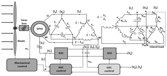
Figure 1.
The considered system of DFIG generator of a wind turbine in islanded grid operation.
The equations of the system in Figure 1 are derived using the symbolic calculations in Matlab R2021b. This new Matlab version has new functions to work with symbolic matrixes (e.g., symmatrix2sym()), which are appropriate for this aim. It is assumed that the mechanical system of a wind turbine ensures the work with the set rotational speed of the DFIG generator rotor ωr. The aim is to determine the system control in the form of voltage . This voltage should be computed in the RSC control subsystem. The rotor-side converter (RSC) subsystem is to generate this voltage at the DFIG generator’s rotor terminals. The purpose is to obtain a sinusoidal, three-phase, symmetrical voltage on the terminals of the islanded grid load (Ra, Rb, Rc, La, Lb, Lc). The load is of the RL type; however, the load values are variable, unpredictable and different for each phase. In spite of that fact, the voltage should ideally contain only basic harmonics; higher harmonics, which might be harmful, should be reduced. Continuous time differential equations of the system in Figure 1 are derived with the solve() function from the symbolic calculations toolbox in Matlab. The call to this function is of the form S = solve(eqn1,eqn2,…,eqnM,var1,var2,…,varN); where the ‘eqns’ are symbolic expressions, equations or inequalities, and the ‘vars’ are symbolic variables specifying the unknown variables. The equations of the system should be passed as function parameters together with the variables, the derivatives of which are to be obtained. These derivatives are then returned by functions as elements of the output structure S. While describing the system in Figure 1, the turns ratio of the transformer ζ should be taken into account:
where zs and zt are the number of turns in the transformer winding, connected in star and triangle connections, respectively.
Including the star/triangle connection of the transformer winding, the currents of this transformer can be described in a stationary system a, b, c:
where matrix T is
The description of the system in Figure 1, formatted for the function solve (), begins with equations of the circuit of stator and rotor of the DFIG generator in the dq system:
where
- Rs—resistance of stator winding,
- Ls—inductance of stator winding,
- Lm—magnetizing inductance,
- Rr—resistance of rotor winding,
- Lr—inductance of rotor winding,
- ωs = ω0—synchronic speed (angular frequency),
- ωr—rotor’s rotational speed,
- Vgd + j⋅Vgq—components d and q of the stator voltage in complex notation,
- igd + j⋅igq—components d and q of the stator current in complex notation,
- Vrd + j⋅Vrq—components d and q of the rotor voltage in complex notation,
- ird + j⋅irq—components d and q of the rotor current in complex notation,
- pigd + j⋅pigq—time derivative of the stator current in complex notation,
- pird + j⋅pirq—time derivative of the rotor current in complex notation.
The equations above are passed into the solve () function, separately for the real and imaginary parts, creating a set of first four equations. The capacitors and the primary side of the transformer are connected to the generator terminals (u, v, w), both forming a delta connection. The equations for the voltages on capacitors , which are simultaneously the voltages of u, v, w phases of the generator, are presented below:
These are the equations in stationary phase coordinates for the generator’s voltages , generator’s currents and the currents of the secondary side of the transformer . The equations are turned into rotating coordinates d, q, 0 with the use of Park transformation:
Additionally, the left side of these equations is modified:
where
To the set of equations passed into the function solve (), only the first two equations from (9) concerning d and q coordinates are taken, forming Equations (5) and (6). Equations (7)–(9) are load voltage equations. These equations in phase coordinates are expressed as follows:
These equations are transformed to coordinates d, q, 0:
where .
Equations (10)–(12) describe the triangle/star transformer in Figure 1. In the phase coordinates a, b, c, these equations are
These equations are transformed to d, q, 0 coordinates with the use of Park transformation:
where .
The last Equations (13)–(15) concern the load. In the phase coordinates, they are
After transforming into d, q, 0 coordinates, they are
where
When the equations above are passed to the solve() function, the variables according to which these equations are to be solved should also be given:
These are the derivatives of the state variables describing the system in Figure 1. Under their names herein is the equation number which they form. The state variables are
It is assumed that the control variables are the DFIG’s generator rotor voltages generated by RSC: .
The solutions regarding the variables (18) are given by the solve() function. The obtained equations for variables (18) are continuous time differential equations in the form of
The dimension of this problem is n = 15. The further consideration involves discrete differential equations. The time step dt is assumed. When applying symbols and for state variables in the next step ‘n’ and current step ‘p’, the approximation is obtained:
The formula presented in Equation (21) is not fully implicit. With certain generator and system parameters, the differential equations may become equations of the stiff type. In order to avoid numerical instability, fully implicit methods were also used ref. [39]. Then, the discrete differential equations become stable, and calculations can be performed with a larger time step dt.
After substituting these approximations into Equation (20), the discrete version is obtained.
The obtained equations simulate the examined system in Figure 1. By applying this implicit method of discretization (21), it is possible to avoid instability in numerical solutions. The unknown, random variable load of the system is modeled by applying random changes in resistances Ra, Rb, Rc and inductances La, Lb, Lc in time.
3. The Applied Method of Optimal Control with a Square Cost Function
The purpose of the control system is to provide symmetrical, three-phase voltage at the terminals of the islanded load in Figure 1. Having continuous differential equations of the object (20), the issue can be narrowed to minimizing the cost function e(t) ref. [1,9]:
where T is the end time of the process under consideration, and μ represents the time of integration. The Hamiltonian of the issue can be written as ref. [2,9]
where p is a derivative of cost function e(t) with respect to variables .
In order to obtain the optimal control for minimization of the cost function (23), the conditions of Pontriagin’s equation must be fulfilled [9]. It is assumed that Hamiltonian (24) reaches its minimal value for optimal control :
There is a two-border issue, as the initial conditions for are given for the beginning of the process under consideration t = 0, where the initial conditions for p are given for the end of the process t = T. Thus, it is complicated to solve. However, for the assumed linear state Equation (20), these difficulties can be avoided.
In order to solve it, it is necessary to introduce matrix which relates state variables with vector :
By differentiation, the following expression is obtained:
This is a nonlinear, matrix differential equation, called the Riccati equation. A problem with an infinite time horizon is assumed, where T→∞. Then, the time t, in which Equation (27) is calculated, is unrecognizable regarding the end of process T. This leads to
and to the nonlinear matrix Riccati equation,
and, finally, to optimal control:
The described dependencies apply for the continuous differential equations. In this article, the discreet form of Equation (22) is used. The continuous approach to Equation (20) and the discrete one for Equation (22) are strictly linked. In order to obtain the optimal control for Equation (22) in the calculations, a Matlab function [K,S,CLP] = dlqr(A,B,Q,R,N) is used. This function calculates the optimal matrix K, the solution S of Riccati Equation (29) and the eigenvalues CLP of the system with feedback with the matrix: .
4. Control System Equations
A state variable vector z is used for control. The first n = 15 variables of this state vector z are the variables of the system of type (22). This system, created for control purposes, differs from the system of Equation (22) describing the controlled object in terms of parameter values. Particularly, the islanded load values cannot be given ‘a priori’. In the system of Equation (22) describing the controlled object, the asymmetric, random nature of the load is simulated by loading each phase with a series RL network (Ra, La; Rb, Lb; Rc, Lc) with element values varying randomly over time. The purpose of the RSC control system is to provide a symmetrical three-phase voltage on the islanded grid terminals despite unknown variations in its asymmetrical load. A symmetrical RL load has to be assumed in the control system equations. The values of this load, resistance Roabc and inductance Loabc, the same in each phase, are assumed to correspond to the average load of the system. These values can be estimated during the calculations to better represent the current load on the system. However, as the simulations have shown, the values of the Roabc and Loabc parameters do not have much impact on the proper operation of the control system. This way, the system of equations of type (22) is created but for controlling purposes. If the first n = 15 of the state vector z is denoted as , this system can be written as follows:
In the above formula, the control variable is the rotor voltage generated by the RSC system. For further calculations, it was assumed that the control variable is the rotor current but in the next time step. This way, it is easier to ensure that this current does not exceed the rated value. For this purpose, Equations (5) and (6) are extracted from Equation (31). These equations determine the value of the current :
From these equations, the voltage is calculated, which is then substituted back into Equation (31), obtaining
where .
In order to improve the system’s performance, the dynamic model described by Equation (33) is supplemented with additional equations, closely related to the control. They determine the auxiliary vector of variables . These are discrete differential equations that include the voltage reference of the created islanded grid and the higher error harmonics of that voltage. The number of calculated harmonics was assumed to be il_h = 12. The first harmonic is the fundamental harmonic of voltage , which should not be reduced because it represents the voltage reference . The remaining harmonics are the error harmonics, that is, the harmonics of the difference between the reference and the current voltage (variables x(7:8) from state variables (19)). These error harmonics are subjected to suppression. There are four equations for each harmonic; thus, the number of additional equations for variables is . The total number of variables used for control is then , where n = 15 is the dimension of the problem (22). The selected numbers of the calculated harmonics are
Voltage error harmonic numbers carry a ‘+’ or a ‘−’ sign. Negative numbers refer to the harmonics that create a magnetic field rotating in a direction opposite to the assumed direction of the rotor rotation. It is known that the harmonics with numbers , where k is the integer number, create a field rotating in the positive direction, but harmonics create a field rotating in the negative direction. The list of load voltage harmonic numbers to be suppressed should include the harmonic of number −1. This is the number of the voltage symmetrical component with the opposite direction of rotation. On the other hand, the considerations are made in the dq coordinates rotating in the positive direction with the speed of ωs = ω0. Thus, this set of the harmonics (34) has numbers reduced by 1:
In this situation, the fundamental harmonic in the dq system rotates at a very low speed, which was assumed for stability reasons. This does not generate problems, and the value of voltage can be corrected during computations. The equations for the additional variables are first created in the continuous version:
where the error of the islanded grid voltage is a column vector:
where ‘n’ symbols indicate the value in the next time step. The first four equations of (36) describe the voltage They generate this reference voltage; thus, a part of matrix that corresponds to these equations equals zero. These equations are of the following form (38):
where is a zero matrix sized (2 × 2). Accordingly, is a unit matrix sized (2 × 2), and is the basic angular frequency of the created islanded grid. The equations of the reference voltage generator above are not dependent on the error ; however, they require initial values. Among the four values describing the islanded grid reference voltage ni(1:4), the first two are the d and q components of this voltage, and the other two are the time derivatives of these components. That is why the initial values were taken as
where is the assumed maximum value of the phase voltage of the created grid. The rest of the equations for the additional variables of the system (36) are supposed to isolate harmonics with numbers out of the voltage error (37) on the islanded grid terminals (in dq system). Thus, for instance, for the l-th subsequent number the h-th harmonic is described by an equation of the following form:
The fragments of matrixes given here, should be successively substituted into Equation (36). Equations (38) and (40) are sets of four equations, which form two separate parts, both for d and q components. The first and the third equations are the common part of the d component of the harmonic numbered h from the error . Similarly, the second and fourth equations are the equations for the q component, for the same h-th harmonic of the error . Taking into consideration the d component, namely the first and third equations from (40), the Laplace transform of the variable can be calculated (for the d component):
where is the Laplace transform of the ee error. According to this Equation (41), the system (40) is a filter. This filter isolates the mono-harmonic signal with the angular frequency of with a gain equal to infinity. The rest of the harmonics, except for the h-th one, are suppressed through this filter. Each consecutive set of four equations allows one to isolate the next h-th harmonics in the same way. These harmonics are isolated so that they can be reduced by incorporating them into the process cost function (23). The size of the combined Equations (33) and (36) is . The system of continuous time differential Equation (36) must be transformed to a discrete form. For this purpose, as in the case of Equation (20), an implicit differentiation scheme given by Equation (21) is used. In this way, the possibility of numerical instabilities in the resulting equations is avoided. As a result, a stable system of discrete equations is obtained from Equation (36):
In Equation (42), just as in Equation (37), it is highlighted that the error should be calculated for the next time step ‘n’ and not for the current time step ‘p’. The idea is to reduce the error in the next time step (‘n’), since the error in the current time step ‘p’ cannot be affected. The control variables z consist of variables (Equation (33)) and of (Equation (42)) as
Equation (33) should be combined with Equation (42):
where a two-line matrix w creates an error according to Equation (37), from the vector . This means that it contains zeroes, except for position in the first row and in the second row, where the value is +1. Similarly, for position 7 and 8 in the second row, the value is −1. Furthermore, expressions containing are moved to the left-hand side of Equation (44), and the state Equation (45) for the RSC control system is derived:
It is necessary to create matrices Q and R, which will be used to determine the square cost function E. For a discrete system (45), the equation for this function E takes the following form:
The matrix R limits the value of the control variables, making the second term of Equation (46) competitive to the first term. It is assumed that
The coefficient was assumed for calculations. While creating matrix Q, the error ee has to be taken into account together with the higher harmonics of this error. The value of is applied from Equation (44) with the matrix w, and the higher harmonics of the error placed in vector from (43). To this end, an auxiliary matrix QQ is created. This is a zero matrix of dimension containing the matrix w from Equation (44) in rows and . After multiplying this matrix by vector , an error of voltage of the islanded grid is received on positions and . The square of this error is obtained by
where is a coefficient. The matrix Q is created by adding the contributions of error higher harmonics to . Selected numbers of harmonics are given in (34); the values of these harmonics are in vector . The reference voltage placed for both d and q components on and positions of vector is not considered here. The d and q component values of voltage error higher harmonics should be applied. For instance, the d and q components of the i-th harmonic are placed, respectively, on and positions in vector . This implies that the zero matrices sized should be added to the matrix Q created previously, where the former have a unit matrix, sized , placed in a square contained between lines and columns on the diagonal. Each of these matrices is multiplied by an appropriate coefficient. The coefficient assumed for simulation is inversely proportional to the square root of the harmonic number from (34).
5. Simulations
As it can be seen in Figure 1, the RSC control system uses the measurements of an actual object, simulated here by Equation (22). The measurements of the load voltage , load current , DFIG stator current and DFIG rotor current were used in the simulation. The d and q components of these quantities from the vector x of (19) were placed in the corresponding places in the vector z of Equation (43). Other sets of measurement variables were also tested successfully. The adopted control method allows one to control the value of the rotor current of the DFIG machine so that it does not exceed the rated value. The rotor current is used here as the control variable (Equations (32) and (33)). The maximum nominal value , which should not be exceeded, is assumed:
The current is a control variable for system (45). It is calculated, similarly as in (30), by the function dlqr():
The obtained value is tested with (49) and possibly limited. If the condition (49) is not met, the two components of the vector are proportionally reduced. Thus, the direction of the vector does not change. By having the control current value , the DFIG rotor voltage can be calculated from Equation (32). This voltage has to be generated by the RSC system. The value of this voltage is also tested so that it does not exceed RSC capabilities, determined by the capacitor voltage from Figure 1:
If this condition is not fulfilled, the vector should be reduced, as in the case of the vector , while preserving its direction. In this case, Equation (32) should be applied again to calculate the current . This new, corrected control vector then allows for the calculation of the next time steps, e.g., from Equation (33). In system (22), simulating the real system, the voltage vector is used for this purpose. The matrix R from the cost function formula E (46) also has its limiting effect on the control vector values. However, this possibility was not used here. Constraints (49) and (51) have a large influence on the waveforms. When assuming large values of constraints, e.g., the voltage waveforms on the islanded network are sinusoidal and harmonic free, as can be seen in Figure 2.

Figure 2.
Waveforms of the islanded grid phase voltages and load current .
Highly distorted islanded grid currents were adopted. These currents were obtained by varying the values of load resistance and inductance over time. The waveforms of these values are shown in Figure 3.
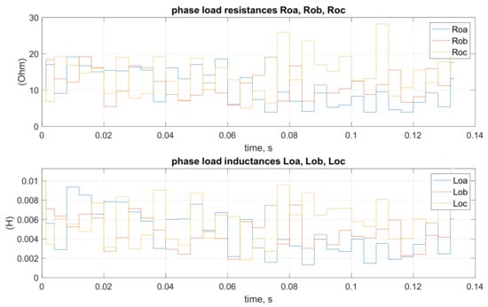
Figure 3.
The resistance and inductance waveforms of the load phases of the islanded grid used in the simulation shown in the figure.
The function dlqr() (50) also determines the eigenvalues E_ of process (45) with the closed feedback loop (50). The eigenvalues of this closed-loop control system are shown in Figure 4. The moduli of these eigenvalues are less than 1, which confirms the stability of the proposed method.

Figure 4.
The eigenvalues of a closed loop RSC control system from Figure 1.
The specification and parameters of the DFIG generator and of the system supplying the islanded grid are given in Table 1.

Table 1.
Specification and parameters of the DFIG generator and of the system supplying the islanded grid.
The purpose of this paper was to verify the performance of the system and its control under difficult conditions when operating in an islanded grid. One aspect of these tests was the assumption of a low generator stator voltage and a sufficiently large transformer ratio. At the same time, a response is provided for the possible exceeding of the generator ratings (49, 51). As seen from the simulations carried out in this chapter, despite these extreme voltage and load conditions, the system behaved correctly.
The set of DFIG generator waveforms is presented in Figure 5.
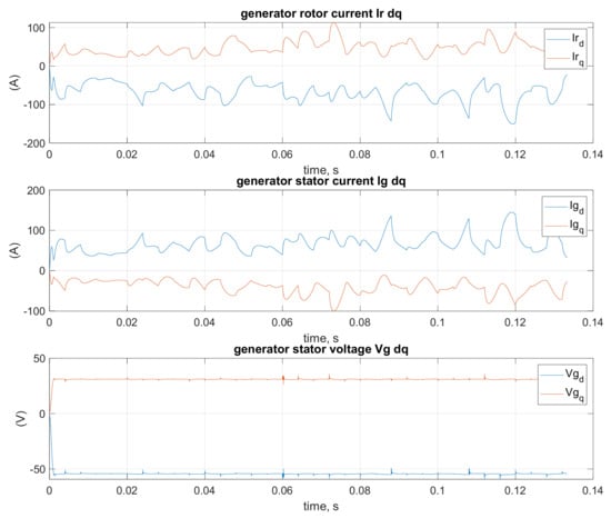
Figure 5.
Stator voltage and stator and rotor currents and of the DFIG generator in dq coordinate system.
In response to the changes in load current caused by the change in load resistance and inductance from Figure 3, the control system responds by changing the rotor supply voltage . The waveforms of these parameters and variables are shown in Figure 6.

Figure 6.
The voltage , powering the rotor, generated by the RSC in the dq coordinate system, against the changes in resistance of the load phases in the islanded grid.
Figure 7 presents the obtained islanded grid voltage against the random load .

Figure 7.
Load voltage maintaining symmetry despite random load in the dq coordinate system.
The behavior of the system was studied while imposing limitations on the rotor current and on the rotor voltage . In order to limit these values, Equations (49) and (51) were used. The value of the load side star-connected capacitors was 50 μF. The waveforms are illustrated in Figure 8, Figure 9, Figure 10, Figure 11 and Figure 12.

Figure 8.
Waveforms of the islanded grid voltage and the distorted load current in the dq coordinate system with the applied limitations on the rotor current as well as the rotor voltage .

Figure 9.
Waveforms of load phase resistances and inductances with a steep drop in load at the time of 0.068 s.

Figure 10.
Stator voltage stator current and rotor current with the load from Figure 9.

Figure 11.
The rotor control voltage in the dq coordinate system against the load phase resistance.

Figure 12.
Load voltage maintaining the symmetry with a delay, as a result of limitations during a steep drop in load in Figure 9, expressed by the current .
As can be seen in Figure 8, there is a strong drop in load (Figure 9), to which the system reacts with some delay. This is the result of the imposed constraints.
In Figure 13, Figure 14, Figure 15, Figure 16 and Figure 17, the results are shown with the rotor voltage limitation, , preserved but with the rotor current limitation removed. The value of the capacitor was increased to 100 μF. The response of the system to a steep load change under these conditions is shown.

Figure 13.
Waveforms of load voltage and the distorted load current in the dq coordinate system, with no limitations on the rotor current, limitations on rotor voltage and capacity during steep increase of the system load.

Figure 14.
Waveforms of load phase resistances and inductances with a steep load increase at the time of 0.068 s.

Figure 15.
Stator voltage , stator current and rotor current in the dq coordinate system, with no limitations on the rotor current but with limitations on the rotor voltage under increasing load conditions as in Figure 14.

Figure 16.
The rotor control voltage in the dq coordinate system against the changes in resistance of the load phases in the islanded grid with the voltage limit .

Figure 17.
Load voltage during a steep increase in load current at the time of 0.068 s in the dq coordinate system.
The behavior of the system with imposed limitations, namely, and , during a steep decrease in resistance and inductance of the load, which resulted in an overload of the system, is presented in Figure 18, Figure 19, Figure 20, Figure 21 and Figure 22.
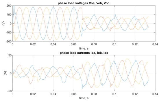
Figure 18.
Waveforms of load voltage and the distorted load current of the in the dq coordinate system with substantial limitations on and and with a steep increase in load for the time of 0.068 s, where the load increase results in the decrease and deformation of the voltage .

Figure 19.
Waveforms of load phase resistances and inductances simulating a steep load increase.

Figure 20.
Stator voltage , stator current and rotor current in the dq coordinate system, with limitations on control values, when the system does not provide appropriate voltage due to overload.

Figure 21.
Rotor control voltage in the dq system, with limitations on control and with changes in the load as presented in Figure 19.
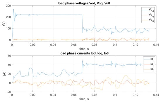
Figure 22.
Load voltage and load current with limitations on control and a steep increase in the load at the time of 0.068 s, when the system does not provide appropriate voltage of the load .
6. Damping of Rotor System Oscillations
The load of an islanded grid varies randomly, differently for each phase. Despite this difficulty, the presented RSC inverter control method ensures the symmetry of the voltages on the load. In order to achieve this objective, the optimal control with quadratic cost function was used. The equations of the system were extended to include the equations for a three-phase voltage reference and to filter selected harmonics of the voltage error at the load compared to the reference voltage. The voltage symmetrization results obtained are satisfactory. However, the occurrence of oscillations in the RSC inverter voltage (rotor side) was observed. In the dq coordinates, these oscillations have network angular frequency. They are generated by the control system to ensure the required symmetry. However, the decay rate of these oscillations is important because they are associated with power flows through the RSC inverter to the supply capacitor. The second important element of the system’s operation is to ensure that the current and voltage of the rotor side do not exceed the ratings. The control variable is the rotor current. When the control requests to increase this current above the rated value, it must not be allowed to do so. In the program, both dq components of this current are equally reduced in order to not exceed the rated value. To maintain both of these objectives, i.e., to accelerate the decay of the grid frequency RSC inverter voltage oscillation (in the dq coordinate system) and to protect against exceeding the rated value of the rotor current, two methods were verified:
- Adding the square of the module of the derivative of the rotor current into the cost function with an appropriate coefficient.
- Extracting the grid frequency oscillations (in the dq system) from the voltage supplied to the rotor and also adding them as the square of the modulus into the cost function with the appropriate coefficient.
The optimization process seeks to reduce the cost function. Therefore, both of the above steps will control the rate of increase of the rotor current , not allowing this current to increase too fast, and, at the same time, they will cause the rotor voltage oscillation to decay faster. Therefore, the power flow through the RSC inverter will be limited in both directions. The circuit that implements these methods is shown in the Figure 23.

Figure 23.
Control system of a wind turbine with a DFIG generator for island grid operation to accelerate the decay of rotor voltage oscillations and rotor current oscillations .
In the presented figure, there is an RLC filter circuit drawn in a dotted line rectangle. This filter does not physically load the voltage but only functions in the control process to isolate the voltage component of the line frequency in the dq coordinate system computationally. This component in the form of current is used in the cost function. The impact of the two proposed methods on the controller operation depends on the coefficients with which their representative values are added into the cost function. Three combinations of coefficients were tested. They are denoted by letters ‘a, b, c’:
- (a)
- Protection for rotor voltage harmonic is on; protection for current derivative is 10 times smaller,
- (b)
- Both protections are on, with almost the same shares in the cost function,
- (c)
- Only the protection for rotor voltage harmonics is on.
The corresponding waveforms are indicated by letters ‘a, b, c’. Figure 24, Figure 25, Figure 26, Figure 27, Figure 28 and Figure 29 show the results of operation of the discussed protections.
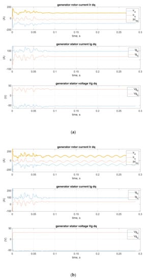
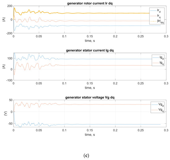
Figure 24.
Dq coordinates of rotor current , stator current and stator voltage of DFIG generator: (a) type a protection is applied; (b) type b protection is applied; (c) type c protection is applied.

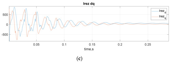
Figure 25.
Fading of current of the grid angular frequency filter of the rotor voltage : (a) type a protection is applied; (b) type b protection is applied; (c) type c protection is applied.
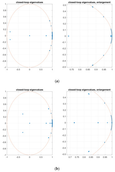
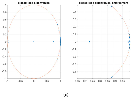
Figure 26.
Distribution of eigenvalues for the closed loop system: (a) type a protection is applied; (b) type b protection is applied; (c) type c protection is applied.

Figure 27.
Active powers of stator Pg, rotor Pr and load Po and reactive powers of stator Qg, rotor Qr and the electromagnetic torque of generator DFIG (* 100) for protection a.

Figure 28.
Waveforms of rotor phase voltages and rotor currents for protection a.

Figure 29.
Load current and generator stator current waveforms in dq coordinates for protection a.
In the presented waveforms, it can be seen how dependent they are on the proper choice of coefficients. It turns out that adding a component from the derivative of the rotor current in the cost function is quite problematic. On the other hand, adding a current of the filter that captures the fundamental harmonic from the rotor voltage in dq coordinates in the cost function contributes to a faster decay of the system oscillations. What is noteworthy is that this current is not actually sourced from the rotor voltage ; it is only used during control. Using the derivative of the rotor current in the cost function is only beneficial if its contribution to the cost function is 10 times smaller than the contribution of the filter current as in the case of a. It limits the rate of increase of the rotor current , with which it contributes to ensuring the rated limits for the current. At the same time, it is associated with correspondingly lower supply and rotor voltages.
7. Conclusions
The optimization method with square cost functions (23) and (46) confirmed its usefulness in the control of a rotor-side converter of a DFIG generator of a wind farm. The main goal was to obtain a three-phase symmetrical voltage with the minimal higher harmonic content for receivers in an islanded grid. The difficulty in gaining such a high-quality voltage is connected to an uneven load on each phase. Additionally, the load of each phase of an islanded grid changes randomly. The cost function is determined by the given matrices Q and R in the cost function (46). The relationship between these matrices is established by etaR and eta1 coefficients from Equations (47) and (48). These coefficients determine the effect of an increase in the control value and the voltage error on the control process. The decay rate of the transients of the state variables is also important. The oscillation in the rotor current in dq coordinates was observed. Successful attempts were made to control these states. In the cost function, the shares of the islanded grid voltage quality, the value of control variables and the decay rate of state variable oscillations have to be balanced. The results are presented in Figure 30. The load in these simulations is variable in nature in the time range up to 0.05 s. After this time, the load is constant. It can be seen how the oscillations of the rotor current , generator current and generator voltage decay.
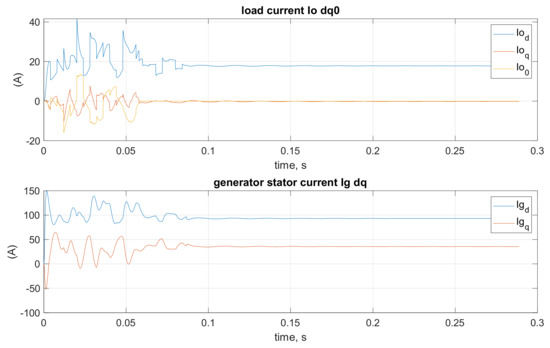
Figure 30.
Oscillations of rotor current , generator current and generator voltage in dq coordinate system.
The above considerations were carried out assuming a constant speed of the turbine. The turbine system is responsible for speed stabilization. However, when the speed of the wind turbine assembly changes, the proposed optimal control method also works well. The speed changes are slow compared to the electrical process in the system shown in Figure 1, where the calculations are performed with a time step of 10−4 s. However, both the array of state variables (45) and the gain matrix K_st from Equation (50) must be refreshed with each velocity change. Exemplary waveforms of power and electromagnetic torque with a change in rotor speed are shown in Figure 31.

Figure 31.
Active power of stator Pg, rotor Pr and load Po and reactive power of stator Qg, rotor Qr and electromagnetic torque of DFIG generator (* 100) for protection a, at variable rotor speed wr (* 10).
The value of the control variable together with the value of the rotor generator voltage has to be monitored according to (49) and (51). If the maximal values are exceeded, it is recommended to reduce these variables in such a way that both components, d and q, are proportionally reduced. It should be noted that the described method of limiting the rotor current increase by including its increments in the Q matrix of the cost function E of Equation (46) contributes to the preservation of constraints (49) and (50).
The authors see the need for further research in the following areas:
- Further investigation of oscillations in the system caused by random asymmetrical load changes and development of methods for their suppression,
- Development of a method for synchronization of the system under investigation with the grid after normal operation is restored,
- Development of methods of cooperation of several such systems to work in one islanded grid,
- Development of a control system for the tested system to cooperate with a stiff grid,
- Cooperation of the tested system with a weak grid,
- Investigating the possibility of improving the voltage at the terminals of the islanded load Vo by additionally applying the three-phase seventh harmonic (or fifth harmonic) star-connected passive filters at the output of the system, with R, L and C elements tuned to the appropriate frequency.
The purpose of this paper was to test the possibility of the control of a complex system with a DFIG generator, with a large number of variables under difficult operating conditions in an islanded grid. Optimal control made it possible to avoid additional simplifying assumptions. This resulted in good control quality manifested by symmetrization of the three-phase voltage applied to the islanded grid. The presented method made it possible to detect and suppress higher harmonics of given numbers appearing in the output voltage. A list of higher harmonic numbers to be removed was assumed. Prospective studies will allow even more in-depth investigation of the capabilities of the system under different operating conditions. This will enable the authors to construct a physical model of the system under investigation and to conduct experimental studies.
Author Contributions
Conceptualization, L.G. and M.G.; methodology, L.G.; software, M.G. and B.K.; validation, M.G. and B.K.; formal analysis, L.G. and M.G.; investigation, L.G., M.G. and B.K.; resources; data curation, M.G. and B.K.; writing—original draft preparation, M.G. and B.K.; writing—review and editing, M.G. and B.K.; visualization, M.G.; supervision, L.G.; project administration, L.G. and M.G.; funding acquisition, L.G., M.G. and B.K. All authors have read and agreed to the published version of the manuscript.
Funding
This project is financed by the Minister of Education and Science of the Republic of Poland within the “Regional Initiative of Excellence” program for years 2019–2022. Project number 027/RID/2018/19, amount granted 11 999 900 PLN. The article was presented during 16th International Conference Selected Issues of Electrical Engineering and Electronics WZEE 2021 (Rzeszow September 2021).
Institutional Review Board Statement
Not applicable.
Informed Consent Statement
Not applicable.
Data Availability Statement
Not applicable.
Conflicts of Interest
The authors declare no conflict of interest.
References
- Gołębiowski, L.; Lewicki, J. Electromagnetic Systems in Power Electronics; Oficyna Wydawnicza Politechniki Rzeszowskiej: Rzeszów, Poland, 2012. (In Polish) [Google Scholar]
- Gołębiowski, L.; Gołębiowski, M. Electrical Circuits; Oficyna Wydawnicza Politechniki Rzeszowskiej: Rzeszów, Poland, 2012. (In Polish) [Google Scholar]
- Delghavi, M.B. Advanced Islanded-Mode Control of Microgrids. Ph.D. Thesis, The University of Western Ontario, London, ON, Canada, 2011. Available online: https://ir.lib.uwo.ca/etd/297 (accessed on 12 June 2021).
- Yuan, C. Resilient Distribution Systems with Community Microgrids; The Ohio State University: Columbus, OH, USA, 2016; Available online: https://www.researchgate.net/publication/317969135_Resilient_Distribution_Systems_With_Community_Microgrids (accessed on 18 June 2021).
- Demetriou, P. A Real-Time Solution for Intentional Controlled Islanding and Restoration of Power Systems; University of Cyprus: Nicosia, Cyprus, 2017; Available online: https://www.researchgate.net/profile/Panayiotis-Demetriou/publication/327213365_A_Real-Time_Controlled_Islanding_and_Restoration_Scheme_Based_on_Estimated_States/links/5b83acf792851c1e1234b4c5/A-Real-Time-Controlled-Islanding-and-Restoration-Scheme-Based-on-Estimated-States.pdf (accessed on 18 June 2021).
- Bahrani, B. Islanding Detection and Control of Islanded Single and Two-Parallel Distributed Generation Units; University of Toronto: Toronto, ON, Canada, 2008; Available online: https://tspace.library.utoronto.ca/bitstream/1807/17152/1/Bahrani_Behrooz_200811_Master_thesis.pdf (accessed on 3 July 2021).
- Cha, S.T.; Wu, Q.; Zhao, H.; Wang, C. Frequency Control for Island Operation of Bornholm Power System, Energy Procedia; Elsevier: Amsterdam, The Netherlands, 2014; Volume 61, pp. 1389–1393. [Google Scholar]
- Vásquez, J.C.; Guerrero, J.M.; Gregorio, E.; Rodríguez, P.; Teodorescu, R.; Blaabjerg, F. Adaptive Droop Control Applied to Distributed Generation Inverters Connected to the Grid. In Proceedings of the 2008 IEEE International Symposium on Industrial Electronics, Cambridge, UK, 2–30 July 2008. [Google Scholar]
- Lewis, F.L.; Vrabie, D.L.; Syrmos, V.L. Optimal Control; John Wiley & Sons, Inc.: Hoboken, NJ, USA, 2012. [Google Scholar]
- Tian, P.; Li, Z.; Hao, Z. A Doubly-Fed Induction Generator Adaptive Control Strategy and Coordination Technology Compatible with Feeder Automation. Energies 2019, 12, 4463. [Google Scholar] [CrossRef] [Green Version]
- Tian, P.; Hao, Z.; Li, Z. Doubly-Fed Induction Generator Coordination Control Strategy Compatible with Feeder Automation. Electronics 2020, 9, 18. [Google Scholar] [CrossRef] [Green Version]
- Xu, L.; Yao, L.; Sasse, C. Grid Integration of Large DFIG-Based Wind Farms Using VSC Transmission. IEEE Trans. Power Syst. 2007, 22, 976–984. [Google Scholar] [CrossRef]
- Mlakić, D.; Baghaee, H.R.; Nikolovski, S. A Novel ANFIS-based Islanding Detection for Inverter–Interfaced Microgrids. IEEE Trans. Smart Grid 2018, 10, 4411–4424. [Google Scholar] [CrossRef]
- Ulu, C.; Komurgoz, G. Electrical design and testing of a 500 kW doubly fed induction generator for wind power applications. Turk. J. Electr. Eng. Comput. Sci. 2017, 25, 1278–1290. [Google Scholar]
- Dehong, X.U.; Blaabjerg, F.; Chen, W.; Zhu, N. Advanced Control of Doubly Fed Induction Generator for Wind Power Systems; John Wiley & Sons: Hoboken, NJ, USA, 2018. [Google Scholar]
- Colli, V.D.; Marignetti, F.; Attaianese, C. Analytical and Multiphysics Approach to the Optimal Design of a 10-MW DFIG for Direct-Drive Wind Turbines. IEEE Trans. Ind. Electron. 2012, 59, 2791–2799. [Google Scholar] [CrossRef]
- Sourkounis, C.; Tourou, P. Grid Code Requirements for Wind Power Integration in Europe. Science 2013, 2013, 437674. [Google Scholar] [CrossRef] [Green Version]
- Reindl, P.; Kreischer, C. Diskussion aktueller Netzanschlussbedingungen für DFIG-Windenergieanlagen. Essen. Tag.-Tech. Instandhalt. Schäden 2020, 14, 18–19. [Google Scholar]
- Fortmann, J. Modeling of Wind Turbines with Doubly Fed Generator System, 2015th ed.; Springer Vieweg: Wiesbaden, Germany, 2014. [Google Scholar] [CrossRef]
- El-Naggar, A.K. Advanced Modeling and Analysis of the Doubly-Fed Induction Generator Based Wind Turbines. Ph.D. Thesis, University Duisburg-Essen, Duisburg, Essen, 2016. [Google Scholar]
- Nawir, M.H. Integration of Wind Farms into Weak AC Grids; Cardiff University: Cardiff, UK, 2017. [Google Scholar]
- Gomez, L.A.G.; Grilo, A.P.; Salles, M.B.C.; Filho, A.J.S. Combined Control of DFIG-Based Wind Turbine and Battery Energy Storage System for Frequency Response in Microgrids. Energies 2020, 13, 894. [Google Scholar] [CrossRef] [Green Version]
- Bakouri, A.; Mahmoudi, H.; Abbou, A. Modelling and optimal control of the doubly fed induction generator wind turbine system connected to utility grid. In Proceedings of the 2016 International Renewable and Sustainable Energy Conference (IRSEC), Marrakech, Morocco, 14–17 November 2016. [Google Scholar] [CrossRef]
- Yang, L.; Yang, G.Y.; Xu, Z.; Dong, Z.; Wong, K.P.; Ma, X. Optimal controller design of a doubly fed induction generator wind turbine system for small signal stability enhancement. IET Gener. Transm. Distrib. 2010, 4, 579–597. [Google Scholar] [CrossRef]
- Kanellos, F.D.; Hatziargyriou, N.D. Optimal Control of Variable Speed Wind Turbines in Islanded Mode of Operation. IEEE Trans. Energy Convers. 2010, 25, 1142–1151. [Google Scholar] [CrossRef]
- Yazdani, A. Islanded Operation of a Doubly-Fed Induction Generator (DFIG) Wind-Power System with Integrated Energy Storage. In Proceedings of the 2007 IEEE Canada Electrical Power Conference, Montreal, QC, Canada, 25–26 October 2007. [Google Scholar] [CrossRef]
- Vas, P. Sensorless Vector and Direct Torque Control; Oxford University Press: Oxford, UK, 1998. [Google Scholar]
- Madani, S.S.; Abbaspour, A.; Beiraghi, M.; Dehkordi, P.Z.; Ranjbar, A.M. Islanding detection for PV and DFIG using decision tree and AdaBoost algorithm. In Proceedings of the 2012 3rd IEEE PES Innovative Smart Grid Technologies Europe (ISGT Europe), Berlin, Germany, 14–17 October 2012; pp. 1–8. [Google Scholar]
- Cárdenas, R.; Peña, R.; Alepuz, S.; Asher, G. Overview of Control Systems for the Operation of DFIGs in Wind Energy Applications. IEEE Trans. Ind. Electron. 2013, 60, 2776–2798. [Google Scholar] [CrossRef]
- Yang, L.; Xu, Z.; Østergaard, J.; Dong, Z.Y.; Wong, K.P. Advanced Control Strategy of DFIG Wind Turbines for Power System Fault Ride Through. IEEE Trans. Power Syst. 2012, 27, 713–722. [Google Scholar] [CrossRef] [Green Version]
- Brekken, T.; Mohan, N. Control of a doubly fed induction wind generator under unbalanced grid voltage conditions. IEEE Trans. Energy Convers. 2007, 22, 129–135. [Google Scholar] [CrossRef]
- Ekanayake, J.B.; Holdsworth, L.; Jenkins, N. Comparison of 5th order and 3rd order machine models for doubly fed induction generator (DFIG) wind turbines. Electr. Power Syst. Res. 2003, 67, 207–215. [Google Scholar] [CrossRef]
- Wang, Z.; Sun, Y.; Li, G.; Ooi, B.T. Magnitude and frequency control of grid connected doubly fed induction generator based on synchronized model for wind power generation. IET Renew. Power Gener. 2010, 4, 232. [Google Scholar] [CrossRef]
- Bharti, O.P.; Saket, R.K.; Nagar, S.K. Controller design for DFIG driven by variable speed wind turbine using static output feedback technique. Eng. Technol. Appl. Sci. Res. 2016, 6, 1056–1061. [Google Scholar] [CrossRef]
- Naidu, N.K.S.; Singh, B. Experimental implementation of a doubly fed induction generator used for voltage regulation at a remote location. IEEE Trans. Ind. Appl. 2016, 52, 5065–5072. [Google Scholar] [CrossRef]
- Hee-Sang, K.O.; Yoon, G.; Kyung, N.; Hong, W. Modeling and control of DFIG-based variable speed wind-turbine. Electr. Power Syst. Res. 2008, 78, 1841–1849. [Google Scholar]
- Ko, H.S. Supervisory Voltage Control Scheme for Grid-connected Wind Farms. Ph.D. Dissertation, University of British Columbia, Vancouver, BC, Canada, 2006. [Google Scholar]
- Baghaee, H.R.; Mlakic, D.; Nikolovski, S.; Dragicevic, T. Support Vector Machine-Based Islanding and Grid Fault Detection in Active Distribution Networks. IEEE J. Emerg. Sel. Top. Power Electron. 2020, 8, 2385–2403. [Google Scholar] [CrossRef]
- Butcher, J.C. Numerical Methods for Ordinary Differential Equations, 2nd ed.; John Wiley & Sons, Ltd.: Hoboken, NJ, USA, 2008; ISBN 978-0-470-72335-7. [Google Scholar]
Publisher’s Note: MDPI stays neutral with regard to jurisdictional claims in published maps and institutional affiliations. |
© 2021 by the authors. Licensee MDPI, Basel, Switzerland. This article is an open access article distributed under the terms and conditions of the Creative Commons Attribution (CC BY) license (https://creativecommons.org/licenses/by/4.0/).