
Reverse Osmosis Desalination Plants Energy Consumption Management and Optimization for Improving Power Systems Voltage Stability with PV Generation Resources


Abstract
:1. Introduction
2. Modelling and Assumption
2.1. Problem Formulation
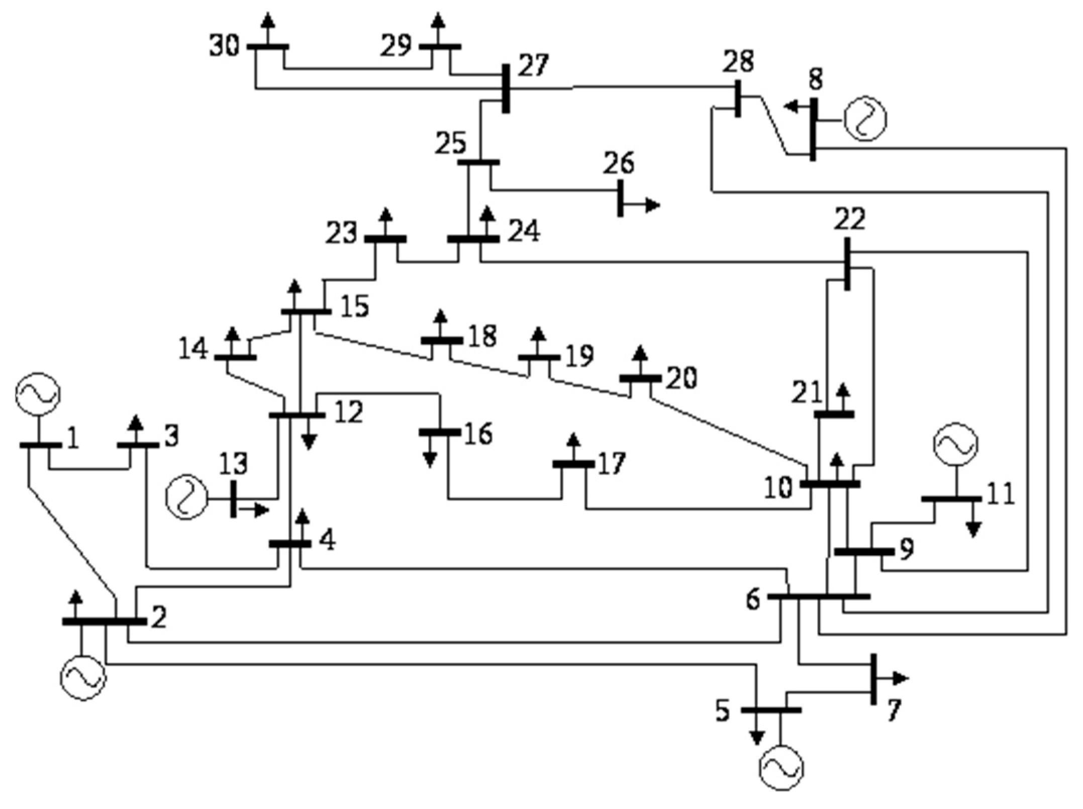
2.2. IEEE 30-Bus System
2.3. Power Flow Study
2.4. PV Power Plants Modelling
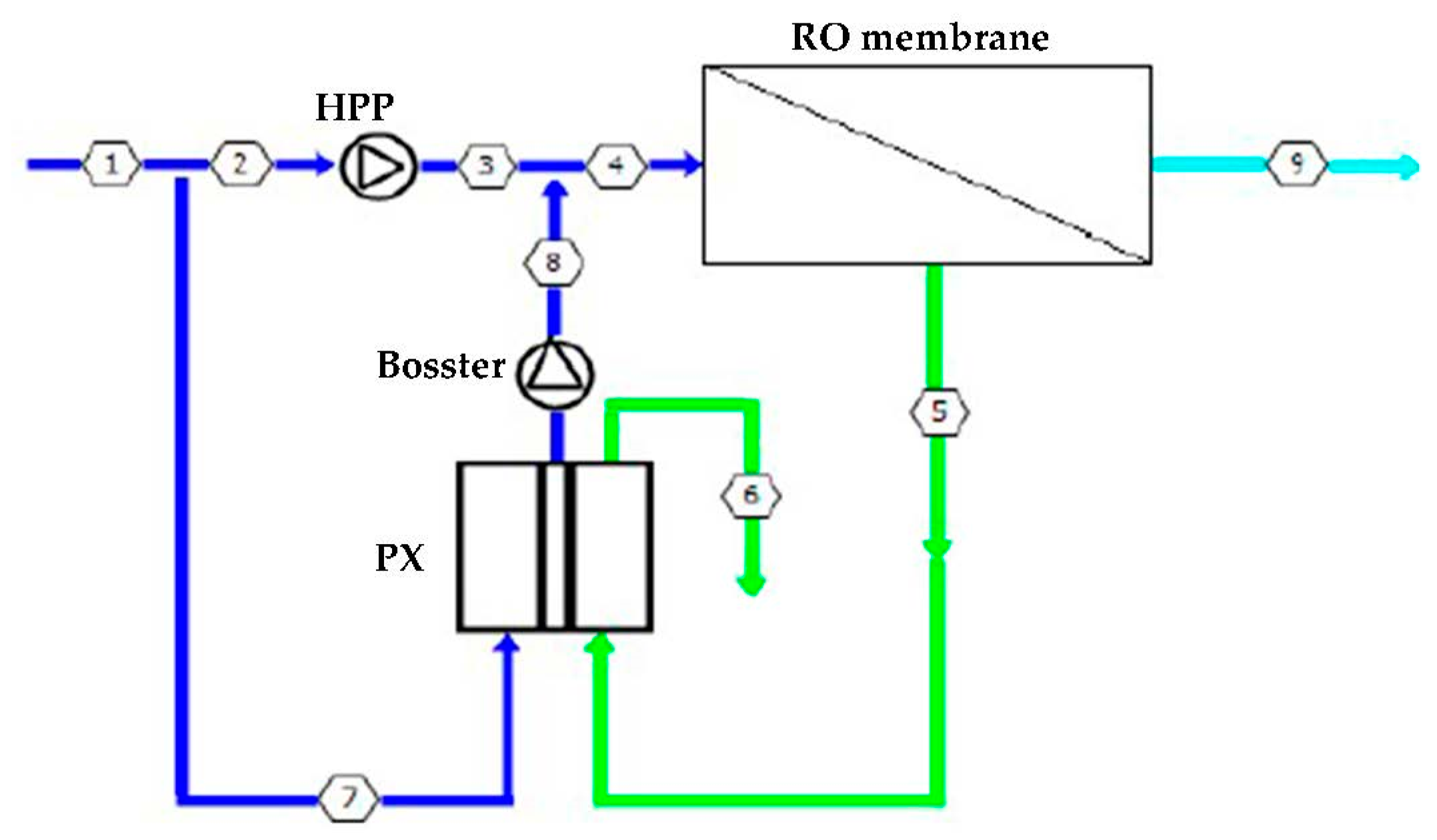
2.5. RO Plant and Energy Consumption Modeling
RO Plants Energy Consumption
- Constant Recovery Ratio Control (CRRC) Scheme
- Variable Recovery Ratio Control (VRRC) Scheme
- The fresh water objective must be maintained at the end of the day so that the water security will not be affected.
- The minimum operating pressure of the HPPs must be higher than the osmotic pressure to prevent back flow.
- The RO trains pressurization and depressurization must be conducted in a controlled way to avoid the mechanical damage of the system. Hydranautics recommends that the RO system be pressurized at no more than 0.69 bar/second to ensure no damage occurs to the membranes. As this study is performed at hourly time basis, this constraint is respected.
- The salinity and temperature of the feed water are constant.
- At any instance, and for safe operation, the RO membrane pressure-temperature limits must not be exceeded. For Hyranautics membranes, the pressure-temperature limits is shown in the following fitted equation [39]:where in bar and T in °C.
3. Results
3.1. Base Case
3.2. RO Plant Integration without Power Consumption Control
3.3. RO Plant Integration with Power Consumption Control
3.3.1. CRRC Scheme
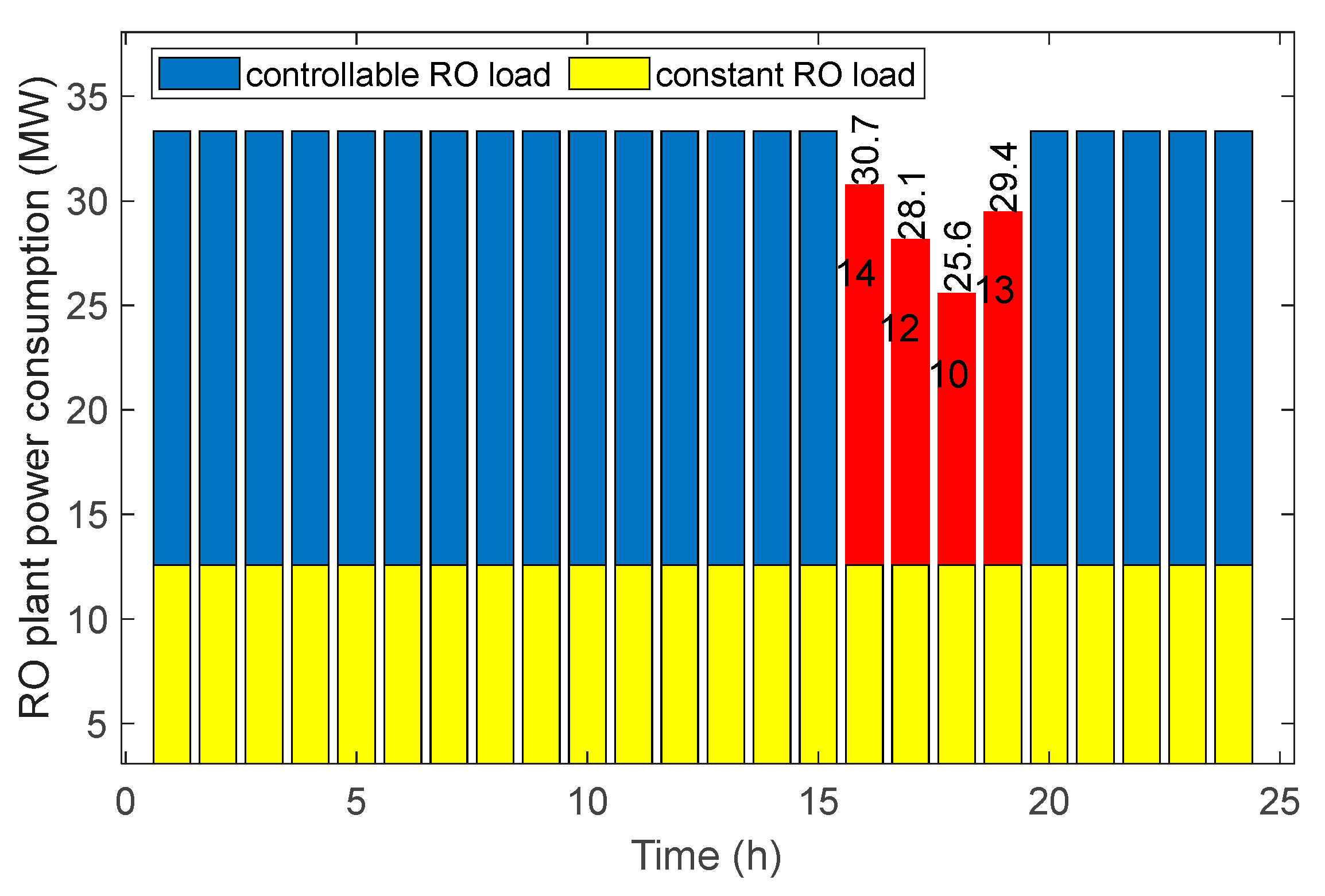
3.3.2. VRRC Scheme
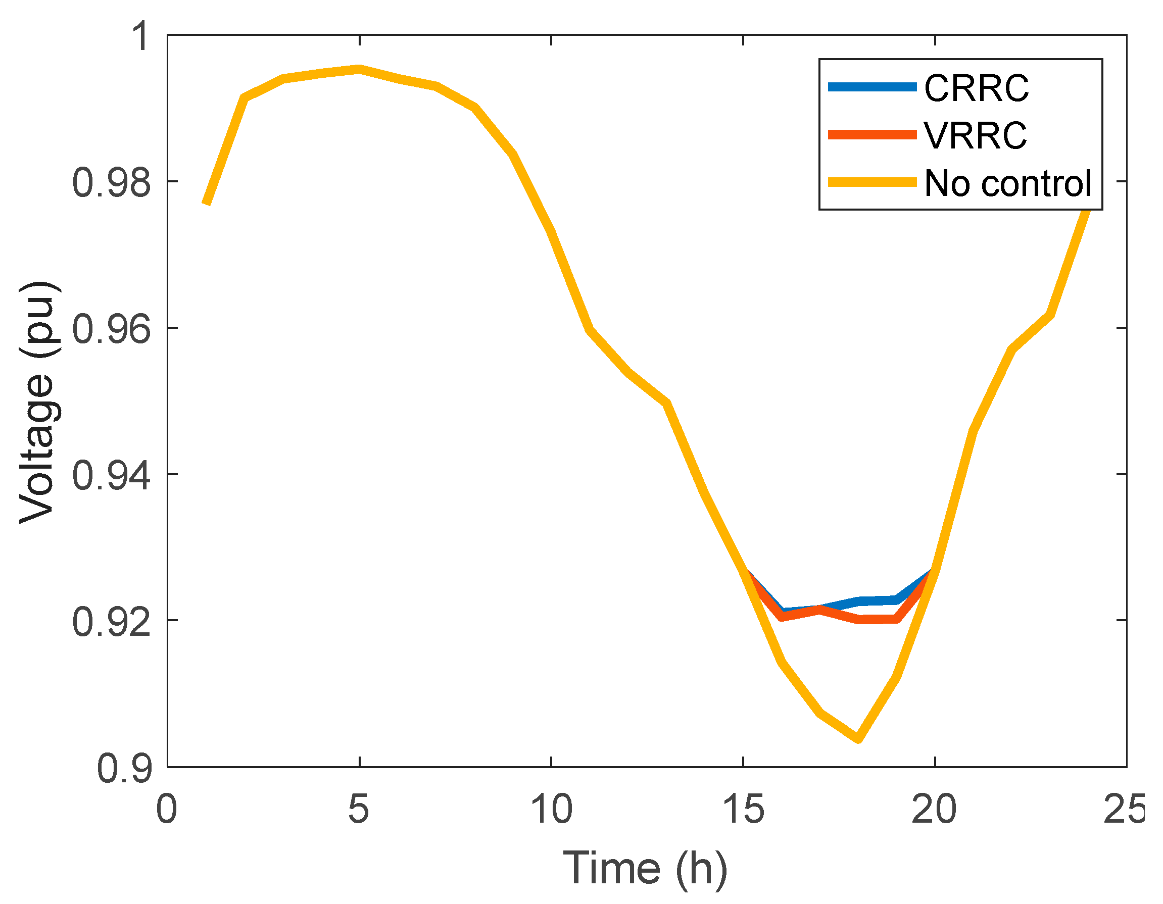
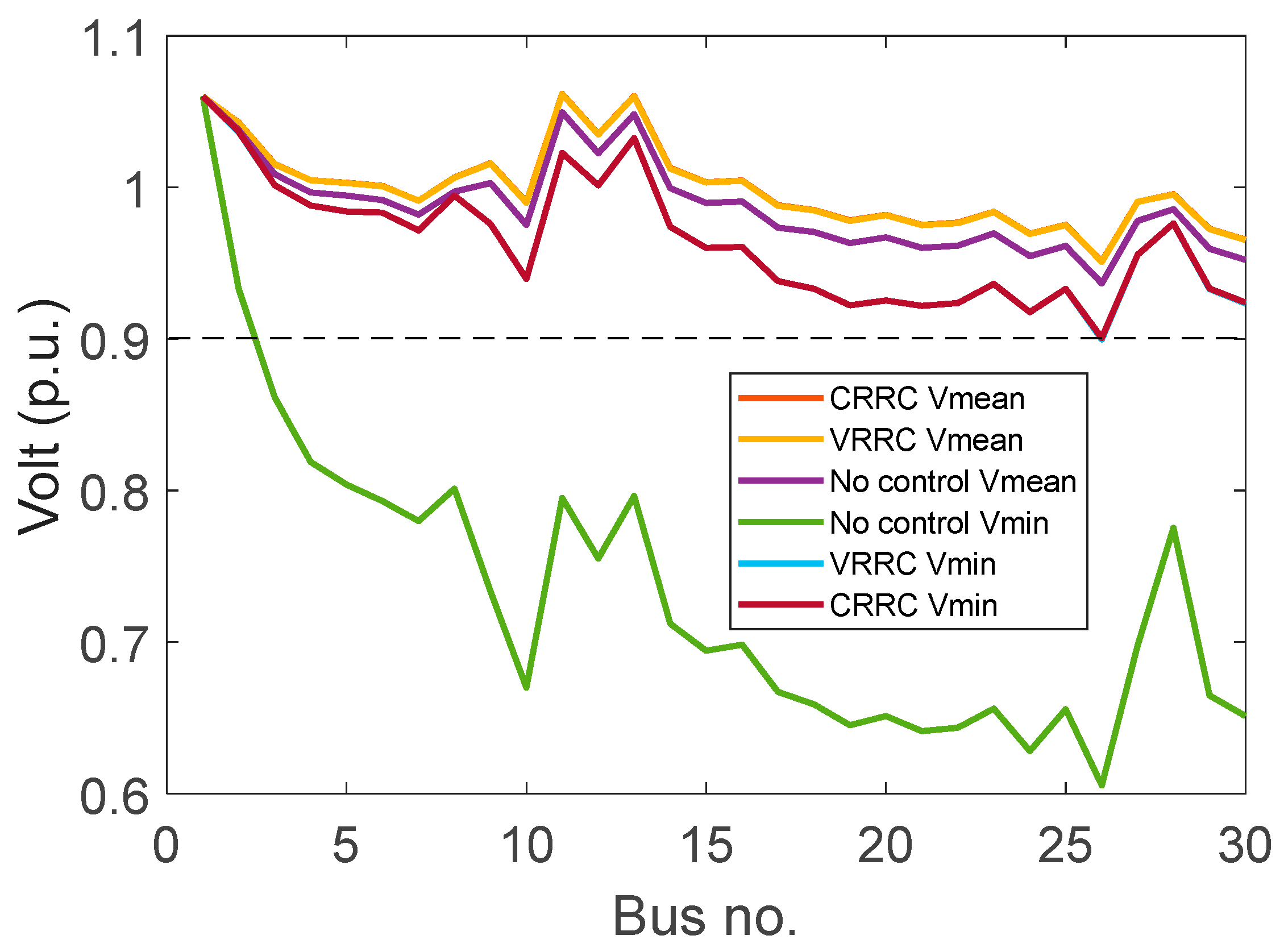
3.4. Comparison between the RO Operational Schemes
3.5. Impact of 5% Increment in Electrical Demand
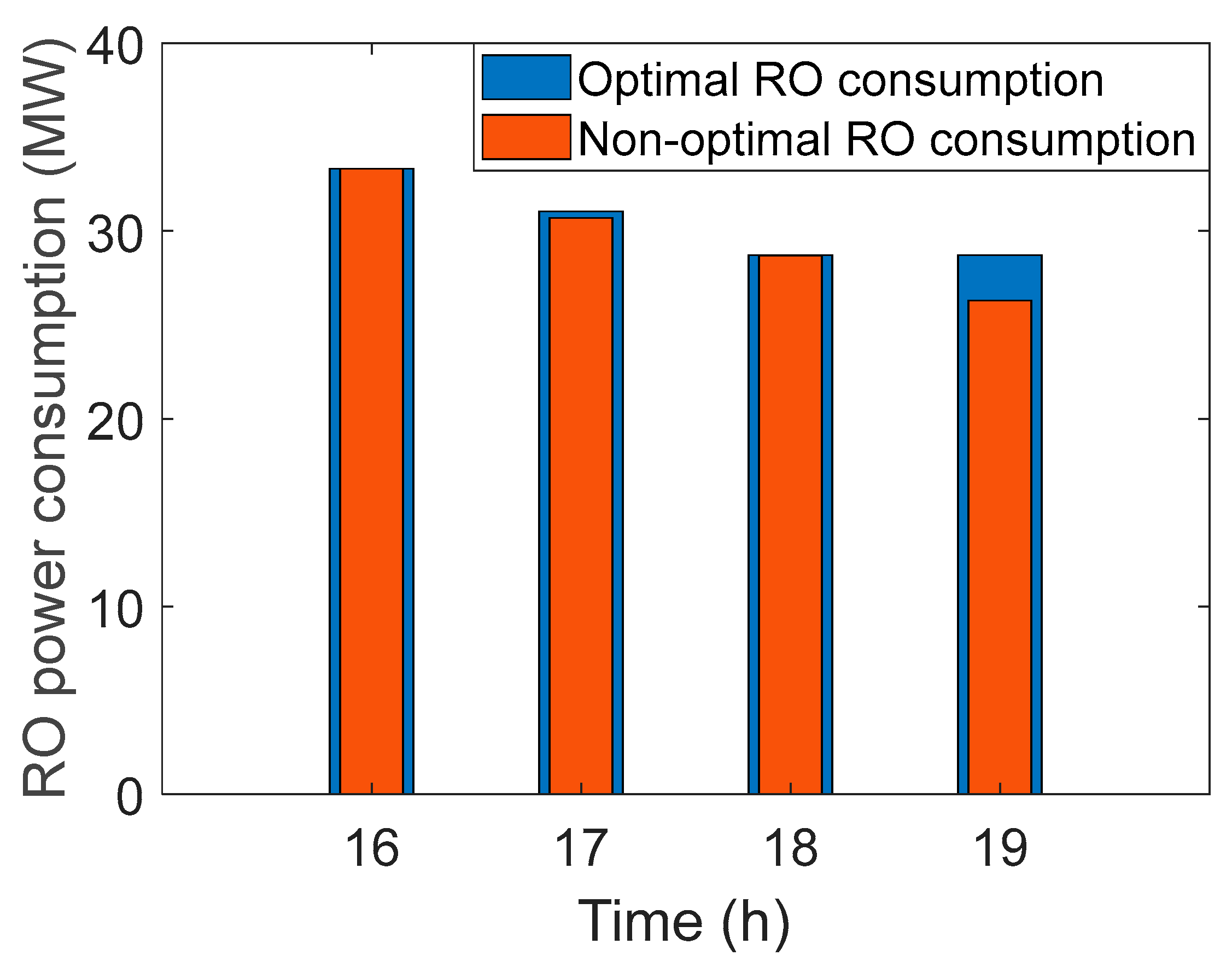
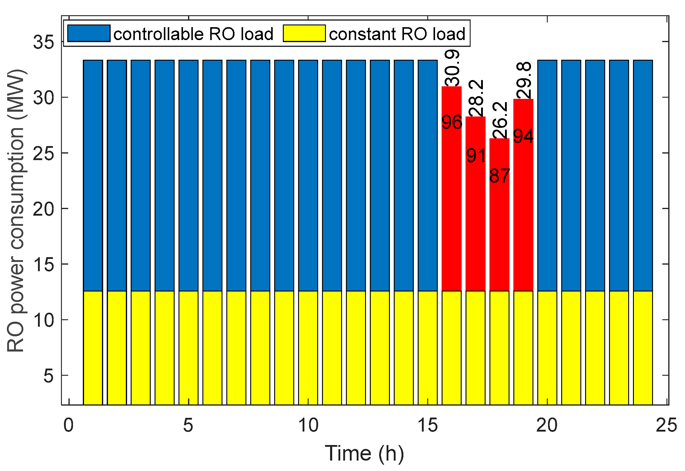
3.6. RO Power Consumption Optimization
4. Conclusions
Author Contributions
Funding
Institutional Review Board Statement
Informed Consent Statement
Data Availability Statement
Acknowledgments
Conflicts of Interest
Nomenclature
| VS | voltage stability |
| PS | power system |
| RO | reverse osmsis |
| SEC | spcefic energy consumption |
| PV | photovoltaic |
| VFD | variable frquency drive |
| RE | renewable energy |
| HPP | high pressure pumps |
| NDP | net driving pressure |
| TDS | total dissolved solids |
| PX | pressure exchanger |
| ERD | energy recovery device |
| CRRC | constant recovery ratio control |
| VRRC | variable recovery ratio control |
| PLAL | Power lines active loss factor |
| PLLF | Power lines loading factor |
| MVA | apparent power flow |
| PG | active power generated |
| MWL | active power loss |
| PSO | particle swarm optimization |
| P | electric active power |
| Q | electric active power |
| voltage | |
| serise resistance | |
| paralell resistance | |
| I | electric current |
| solar radiation | |
| charge of electron | |
| K | Boltzmann’s constant |
| light-generated current | |
| saturation current | |
| pressure | |
| flow rate | |
| f | the ratio of rotational speed/frequency of the centrifugal pumps |
| pump rotational speed | |
| number of RO process working/running units | |
| R | the universal gas constant |
| molar concentration | |
| water transport coefficient | |
| membrane area | |
| permeate flux | |
| recovery ratio | |
| Y | admittance |
| Subscripts | |
| D | demand |
| d | drop |
| l | loss |
| g | generation |
| n | nominal |
| i | bus number |
| j | bus number |
| f | feed |
| I | permeate |
| m | motor |
| P | pump |
| sc | short circuit |
| oc | open circuit |
| Special Symbols | |
| phase angle | |
| efficiency |
References
- Hossain, J.; Pota, H.R. Robust control for grid voltage stability: High penetration of renewable energy. In Power Systems; Springer: Berlin/Heidelberg, Germany, 2014. [Google Scholar]
- Monteiro, M.; de Souza, A.Z.; Lopes, B. The influence of renewable generation in voltage collapse indexes. In Proceedings of the 2017 6th International Conference on Clean Electrical Power (ICCEP), Santa Margherita Ligure, Italy, 27–29 June 2017; pp. 513–518. [Google Scholar]
- Amraee, T.; Ranjbar, A.; Mozafari, B.; Sadati, N. An enhanced under-voltage load-shedding scheme to provide voltage stability. Electr. Power Syst. Res. 2007, 77, 1038–1046. [Google Scholar] [CrossRef]
- Nakawiro, W.; Erlich, I. Optimal load shedding for voltage stability enhancement by ant colony optimization. In Proceedings of the 2009 15th International Conference on Intelligent System Applications to Power Systems, Curitiba, Brazil, 8–12 November 2009; pp. 1–6. [Google Scholar]
- Ahmadi, A.; Alinejad-Beromi, Y. A new integer-value modeling of optimal load shedding to prevent voltage instability. Int. J. Electr. Power Energy Syst. 2015, 65, 210–219. [Google Scholar] [CrossRef]
- Kim, J.S.; Chen, J.; Garcia, H.E. Modeling, control, and dynamic performance analysis of a reverse osmosis desalination plant integrated within hybrid energy systems. Energy 2016, 112, 52–66. [Google Scholar] [CrossRef] [Green Version]
- Novosel, T.; Ćosić, B.; Krajačić, G.; Duić, N.; Pukšec, T.; Mohsen, M.; Ashhab, M.; Ababneh, A. The influence of reverse osmosis desalination in a combination with pump storage on the penetration of wind and PV energy: A case study for Jordan. Energy 2014, 76, 73–81. [Google Scholar] [CrossRef] [Green Version]
- Lienhard, J.H.; Thiel, G.P.; Warsinger, D.M.; Banchik, L.D. Low Carbon Desalination: Status and Research, Development, and Demonstration Needs, Report of a Workshop Conducted at the Massachusetts Institute of Technology in Association with the Global Clean Water Desalination Alliance; Massachusetts Institute of Technology: Cambridge, MA, USA, 2016. [Google Scholar]
- Crainz, M.; Curto, D.; Franzitta, V.; Longo, S.; Montana, F.; Musca, R.; Riva Sanseverino, E.; Telaretti, E. Flexibility services to minimize the electricity production from fossil fuels. A case study in a Mediterranean small island. Energies 2019, 12, 3492. [Google Scholar] [CrossRef] [Green Version]
- Soshinskaya, M. Integrating Renewable Energy Resources: A Microgrid Case Study of a Dutch Drink Water Treatment Plant; Utrecht University: Utrecht, The Netherlands, 2013. [Google Scholar]
- Hummon, M.; Palchak, D.; Denholm, P.; Jorgenson, J.; Olsen, D.J.; Kiliccote, S.; Matson, N.; Sohn, M.; Rose, C.; Dudley, J. Grid Integration of Aggregated Demand Response, Part 2: Modeling Demand Response in a Production Cost Model; National Renewable Energy Lab.(NREL): Golden, CO, USA, 2013. [Google Scholar]
- Atia, A.A.; Fthenakis, V. Active-salinity-control reverse osmosis desalination as a flexible load resource. Desalination 2019, 468, 114062. [Google Scholar] [CrossRef]
- Bognar, K.; Blechinger, P.; Behrendt, F.J.E. Sustainability; Society. Seawater desalination in micro grids: An integrated planning approach. Energy Sustain. Soc. 2012, 2, 14. [Google Scholar] [CrossRef] [Green Version]
- Prathapaneni, D.R.; Detroja, K. Optimal design of energy sources and reverse osmosis desalination plant with demand side management for cost-effective freshwater production. Desalination 2020, 496, 114741. [Google Scholar] [CrossRef]
- Karavas, C.-S.; Arvanitis, K.G.; Papadakis, G. Optimal technical and economic configuration of photovoltaic powered reverse osmosis desalination systems operating in autonomous mode. Desalination 2019, 466, 97–106. [Google Scholar] [CrossRef]
- Lee, S.; Myung, S.; Hong, J.; Har, D. Reverse osmosis desalination process optimized for maximum permeate production with renewable energy. Desalination 2016, 398, 133–143. [Google Scholar] [CrossRef]
- Mohammadi, F.; Sahraei-Ardakani, M.; Al-Abdullah, Y.M.; Heydt, G.T. Coordinated scheduling of power generation and water desalination units. IEEE Trans. Power Syst. 2019, 34, 3657–3666. [Google Scholar] [CrossRef]
- Karakitsios, I.; Dimeas, A.; Hatziargyriou, N. Optimal Management of the Desalination System Demand in Non-Interconnected Islands. Energies 2020, 13, 4021. [Google Scholar] [CrossRef]
- Carta, J.; Gonzalez, J.; Subiela, V. Operational analysis of an innovative wind powered reverse osmosis system installed in the Canary Islands. Sol. Energy 2003, 75, 153–168. [Google Scholar] [CrossRef]
- Torabi, R.; Gomes, A.; Dias, F.M. Demand management for load smoothing in small power systems: The case of Porto Santo island. In Proceedings of the 2019 International Conference in Engineering Applications (ICEA), Sao Miguel, Portugal, 8–11 July 2019; pp. 1–5. [Google Scholar]
- Bognar, K. Energy and Water Supply Systems in Remote Regions Considering Renewable Energies and Seawater Desalination; Shaker: Berlin, Germany, 2013. [Google Scholar]
- Bdour, M.; Dalala, Z.; Al-Addous, M.; Kharabsheh, A.; Khzouz, H. Mapping RO-Water Desalination System Powered by Standalone PV System for the Optimum Pressure and Energy Saving. Appl. Sci. 2020, 10, 2161. [Google Scholar] [CrossRef] [Green Version]
- Ruiz-García, A.; Nuez, I. On-Off Control Strategy in a BWRO System under Variable Power and Feedwater Concentration Conditions. Appl. Sci. 2020, 10, 4748. [Google Scholar] [CrossRef]
- Power Systems Test Case Archive, 30 Bus Power Flow Test Case.
- Villalva, M.G.; Gazoli, J.R.; Ruppert Filho, E. Comprehensive approach to modeling and simulation of photovoltaic arrays. IEEE Trans. Power Electron. 2009, 24, 1198–1208. [Google Scholar] [CrossRef]
- Zarzo, D.; Prats, D. Desalination and energy consumption. What can we expect in the near future? Desalination 2018, 427, 1–9. [Google Scholar] [CrossRef]
- Voutchkov, N. Desalination Engineering: Planning and Design; McGraw Hill Professional: New York, NY, USA, 2012. [Google Scholar]
- Wan, C.F.; Chung, T.-S. Techno-economic evaluation of various RO+ PRO and RO+ FO integrated processes. Appl. Energy 2018, 212, 1038–1050. [Google Scholar] [CrossRef]
- Lobanoff, V.S.; Ross, R.R. Centrifugal Pumps: Design and Application; Elsevier: Amsterdam, The Netherlands, 2013. [Google Scholar]
- Vrouwenvelder, J.; Buiter, J.; Riviere, M.; Van der Meer, W.; Van Loosdrecht, M.; Kruithof, J. Impact of flow regime on pressure drop increase and biomass accumulation and morphology in membrane systems. Water Res. 2010, 44, 689–702. [Google Scholar] [CrossRef]
- Vrouwenvelder, J.; Hinrichs, C.; Van der Meer, W.; Van Loosdrecht, M.; Kruithof, J. Pressure drop increase by biofilm accumulation in spiral wound RO and NF membrane systems: Role of substrate concentration, flow velocity, substrate load and flow direction. Biofouling 2009, 25, 543–555. [Google Scholar] [CrossRef]
- Gu, B.; Adjiman, C.S.; Xu, X.Y. The effect of feed spacer geometry on membrane performance and concentration polarisation based on 3D CFD simulations. J. Membr. Sci. 2017, 527, 78–91. [Google Scholar] [CrossRef]
- Hydranautics. Available online: https://membranes.com/solutions/software-imsdesign/ (accessed on 17 September 2021).
- Hydranautics. SWC4 MAX. Available online: https://membranes.com/wp-content/uploads/Documents/Element-Specification-Sheets/RO/SWC/SWC4-MAX.pdf (accessed on 17 September 2021).
- DUPONT. Tech Manual Excerpt System Operation Initial Start-Up. 2020. Available online: https://www.dupont.com/content/dam/dupont/amer/us/en/water-solutions/public/documents/en/45-D01609-en.pdf (accessed on 17 September 2021).
- International, R.O.C. Reverse Osmosis Plant Shut-Down Procedures. Available online: http://reverseosmosischemicals.com/reverse-osmosis-guides/reverse-osmosis-plant-shut-down-procedures (accessed on 17 September 2021).
- Boda, R. Plant Services Engineering Manager, Hydranautics–A Nitto Group Company; Jebel Ali Free Zone: Dubai, United Arab Emirates, 2020. [Google Scholar]
- VFD versus Control Valve for Pump Flow Controls. Available online: http://www.vfds.org/vfd-versus-control-valve-for-pump-flow-controls-580010.html (accessed on 17 September 2021).
- Company, H.N.G. Technical Service Bulletin, Reverse Osmosis and Nanofiltration Membrane Element Details and Precautions for Use. 2020. Available online: https://membranes.com/wp-content/uploads/Documents/TSB/TSB105.pdf (accessed on 17 September 2021).
- Daily Energy Demand Curve. Available online: https://energymag.net/daily-energy-demand-curve/ (accessed on 17 September 2021).


| Parameter | Value |
|---|---|
| Maximum power Pmax (W) | 250 W |
| Optimum Operating Voltage Vmax (V) | 30.1 V |
| Optimum Operating current Imax (A) | 8.3 A |
| Open Circuit volatage Voc (V) | 37.2 V |
| Short Circuit Current Isc (A) | 8.87 A |
| Pmax Temperature Coefficient | −0.43%/°C |
| Stream No | q (m3/h) | p (bar) | TDS | Econd (µs/cm) |
|---|---|---|---|---|
| 1 | 1042 | 0 | 35,000 | 53,540 |
| 2 | 526 | 0 | 35,000 | 53,540 |
| 3 | 526 | 69.1 | 35,000 | 53,540 |
| 4 | 1042 | 69.1 | 36,099 | 55,122 |
| 5 | 521 | 67.2 | 71,972 | 105,836 |
| 6 | 521 | 0 | 69,754 | 102,741 |
| 7 | 521 | 0 | 35,000 | 53,540 |
| 8 | 521 | 69.1 | 37,218 | 56,732 |
| 9 | 521 | 0 | 188 | 409 |
| VFD Factor | Hour 16 | Hour 17 | Hour 18 | Hour 19 |
|---|---|---|---|---|
| f1 | 0.8 | 0.8 | 0.8 | 0.8 |
| f2 | 0.8 | 0.8 | 0.8 | 0.8 |
| f3 | 0.8 | 0.8 | 0.8 | 0.8 |
| f4 | 0.917 | 0.8 | 0.8 | 0.8 |
| f5 | 1 | 0.8 | 0.8 | 0.89 |
| f6 | 1 | 0.84 | 0.8 | 1 |
| f7 | 1 | 0.87 | 0.813 | 1 |
| f8 | 1 | 0.92 | 0.962 | 1 |
| f9 | 1 | 0.97 | 1 | 1 |
| f10 | 1 | 1 | 1 | 1 |
| f11 | 1 | 1 | 1 | 1 |
| f12 | 1 | 1 | 1 | 1 |
| f13 | 1 | 1 | 1 | 1 |
| f14 | 1 | 1 | 1 | 1 |
| f15 | 1 | 1 | 1 | 1 |
| f16 | 1 | 1 | 1 | 1 |
Publisher’s Note: MDPI stays neutral with regard to jurisdictional claims in published maps and institutional affiliations. |
© 2021 by the authors. Licensee MDPI, Basel, Switzerland. This article is an open access article distributed under the terms and conditions of the Creative Commons Attribution (CC BY) license (https://creativecommons.org/licenses/by/4.0/).
Share and Cite
Haidar, Z.A.; Al-Saud, M.; Orfi, J.; Al-Ansary, H. Reverse Osmosis Desalination Plants Energy Consumption Management and Optimization for Improving Power Systems Voltage Stability with PV Generation Resources. Energies 2021, 14, 7739. https://doi.org/10.3390/en14227739
Haidar ZA, Al-Saud M, Orfi J, Al-Ansary H. Reverse Osmosis Desalination Plants Energy Consumption Management and Optimization for Improving Power Systems Voltage Stability with PV Generation Resources. Energies. 2021; 14(22):7739. https://doi.org/10.3390/en14227739
Chicago/Turabian StyleHaidar, Zeyad A., Mamdooh Al-Saud, Jamel Orfi, and Hany Al-Ansary. 2021. "Reverse Osmosis Desalination Plants Energy Consumption Management and Optimization for Improving Power Systems Voltage Stability with PV Generation Resources" Energies 14, no. 22: 7739. https://doi.org/10.3390/en14227739
APA StyleHaidar, Z. A., Al-Saud, M., Orfi, J., & Al-Ansary, H. (2021). Reverse Osmosis Desalination Plants Energy Consumption Management and Optimization for Improving Power Systems Voltage Stability with PV Generation Resources. Energies, 14(22), 7739. https://doi.org/10.3390/en14227739