Inverse Optimal Control Using Metaheuristics of Hydropower Plant Model via Forecasting Based on the Feature Engineering

Abstract

Optimal operation of hydropower plants (HP) is a crucial task for the control of several variables involved in the power generation process, including hydraulic level and power generation rate. In general, there are three main problems that an optimal operation approach must address: (i) maintaining a hydraulic head level which satisfies the energy demand at a given time, (ii) regulating operation to match with certain established conditions, even in the presence of system’s parametric variations, and (iii) managing external disturbances at the system’s input. To address these problems, in this paper we propose an approach for optimal hydraulic level tracking based on an Inverse Optimal Controller (IOC), devised with the purpose of regulating power generation rates on a specific HP infrastructure. The Closed–Loop System (CLS) has been simulated using data collected from the HP through a whole year of operation as a tracking reference. Furthermore, to combat parametric variations, an accumulative action is incorporated into the control scheme. In addition, a Recurrent Neural Network (RNN) based on Feature Engineering (FE) techniques has been implemented to aid the system in the prediction and management of external perturbations. Besides, a landslide is simulated, causing the system’s response to show a deviation in reference tracking, which is corrected through the control action. Afterward, the RNN is including of the aforementioned system, where the trajectories tracking deviation is not perceptible, at the hand of, a better response with respect to use a single scheme. The results show the robustness of the proposed control scheme despite climatic variations and landslides in the reservoir operation process. This proposed combined scheme shows good performance in presence of parametric variations and external perturbations.

1. Introduction

Hydropower plants management is a problem which complexity is related to the increase of the population on the vicinities of these power generation systems. Taking decisions related to dam volumes and their reservoir of destination poses a real challenge, especially when there are inhabited areas that could be at risk of flooding [1]. Some of the factors involved in dam volumes management include some climatic phenomena, particularly those which may cause landslides and, as a result, changes in storage capacity [2]. Such perturbations in storage capacity are problematic because these cause the system to be unable to satisfy the required energy demand [3], thus, it is necessary to implement techniques to handle said external perturbations and to manage the hydraulic level without hindering power generation or the network’s energy supply.

To tackle this problem, it is necessary to model the dynamics hydropower plant [4,5,6,7], in order to calculate the power generated by the system [8]. Recently, several works related to the power regulation problem in hydropower plants have been published; in [9], for example, an application of a robust controller to regulate the speed of the governor was proposed. Following this trend, in [10] a PID controller that allows one to maximize power generation was developed. Then, in [11], an application for a controller based on passivity was presented.

Due to the complexity involved in the development of an integrated control model which satisfies energy demand while also maintaining the desired hydraulic level, in [5] a new control system is designed by decomposing the dynamic system into subsystems, allowing it to tackle several problematics, including the management of the hydraulic head. To reach a desirable performance in the CLS, in [12,13] the implementation of metaheuristic algorithms were proposed in order to optimize the controller parameters.

Another trait as important as the management of the hydraulic head is trajectory tracking, in which a compromise between ensuring the desired output and the discharge evacuation through landfills are sought after. Several works exist within the literature that are aimed to tackle this problem, especially those that describe the IOC technique as an alternative for referenced tracking, in which a passive system is constructed through the feedback of the output, ensuring its stability, and optimizing its response [14,15,16]. However, despite its good performance, this technique is not suitable in the presence of parametric variations within the system [17]. Furthermore, in [18] an integrator is added to the control scheme to gain robustness to uncertainties. Another challenge when implementing IOCs in the modeling of hydropower systems involves the management of external perturbations modifying the input. With the purpose of solving this problem, in [19] a state observer is proposed to handle these perturbations. In [20] an application of both an adaptable fuzzy controller and IOC is proposed with great success in terms of reference tracking in the presence of external dynamics. Furthermore, in [21], a combination of sliding mode controllers and neural IOC was presented, resulting in a robust scheme even in the face of parametric variations and external perturbations, although modeling of hydropower systems is not implemented. While the previously mentioned works have shown good results in their own right, these drive away from the necessity of ensuring optimal trajectory tracking in hydraulic systems, as identifying external perturbations are required. To tackle this problem, many researchers have proposed the use of artificial intelligence algorithms for prediction. A first approximation is presented in [3], where a chaotic model was described for flow simulation subjected to environmental variations. A better approach is presented in [22], where a Nonlinear Auto–regressive Neural Network (NN) with exogenous input was applied with good results, while in [23] predictions on the flow tendency and its remainder was also implemented to compensate the resulting output, thus reducing prediction error. Due to the previous, NN are attractive for predictions, particularly for a task known as neural forecasting [24]. To allow efficient neural forecasting, Feature Engineering (FE) is a crucial step in the machine learning pipeline [25]. However, there are some issues involved in this methodology, such as loss of information and the presence of noise (spurious data). In [26] several data input approaches based on Nearest Neighbor criterion where presented. Then, in [27,28] some techniques based on averaged noise filter for time series are presented. In [29] some criterions aimed to measure statistics anomalies are presented; however, the use of these techniques requires measuring distances and also need the implementation of several data transformations to normalize data [30] and correct the bias related to historical data [31].

Contribution and Organization

In this research, a robust IOC scheme with an RNN is applied to the HP system. The control is adjusted through the Particle Swarm Optimization (PSO) algorithm [32], and the data for the neuronal predictor is worked with FE. The objective of this work is to track a reference to hydraulic head and mechanical power with an unknown flow rate depending on the weather. The main contribution of this paper is to incorporate an accumulative gain for Inverse Optimal algorithm to attenuate the parametric variations and include a NN to forecasting the external disturbance. Also, to train the NN, the historical data is pre-processed using FE methods.

To achieve the objective presented, it is necessary to obtain a discrete-time model of a reservoir, parsed in Section 2. Then, the Inverse Optimal control with an accumulative action is described in Section 3. Subsequently, the NN structure is deduced and the FE methods are applied to perform the forecasting in Section 4. The general scheme is simulated in Section 5. After that, we present the discussion, results, and their interpretation in Section 6. Finally, the paper is concluded in Section 7.

2. Dynamical Model

Consider the balance flow equation, that describes the variation rate of hydraulic head [4,5,6,7]

$$A\dot{H}=Q_{in}-Q_{out},$$

(1)

where, $Q_{in}$ is the unknown input flow. $Q_{out}=q_s+{\sum }_{i=1}^n{Q}_i$, with $q_s$ as the flow out of spillway and, $Q_i$ as the flow in the duct i, for $i=\{1,2,\dots ,n\}$. Besides, A is the transverse area of the reservoir and H is the hydraulic head level.

Then, an expression to represents the dynamical contribution for flow rate, is obtained from the second Newton law

$$\sum F=m\dot{v},$$

(2)

with the sum of interactions $\sum F=A_{c}H\rho g+A_c{L}_i\rho g\frac{h_b}{L_i}-A_c{h}_i\rho g$, this describes the contribution of the reservoir, the gravity interaction from the duct i, and the opposite force by the pressure in the turbine i, respectively. The mass in each duct is $m=A_c{L}_i\rho$, where $A_c$ is the transverse section of each duct, $L_i$ is the longitude of conduct, $\rho$ and g are the water density and the acceleration by gravitational interaction, respectively. Notice that, the model contemplates that the reservoir must always maintain a minimum level of water. This level has to be greater than the diameter of the cross-section to avoid variations in mass from (2). Whereas, ${\dot{v}}_i=\frac{{\dot{Q}}_i}{A_c}$ correspond to the derivative of velocity water. Then the flow dynamics is depicted as follows

$${\dot{Q}}_i=\frac{A_{c}g}{L_i}(H+h_b-h_i).$$

(3)

Consider also, the energy balance proposed by the Bernoulli equation

$$\frac{\mathsf{\Delta }P}{\rho }+\mathsf{\Delta }Hg+\frac{1}{2}\mathsf{\Delta }{v}^2=0$$

(4)

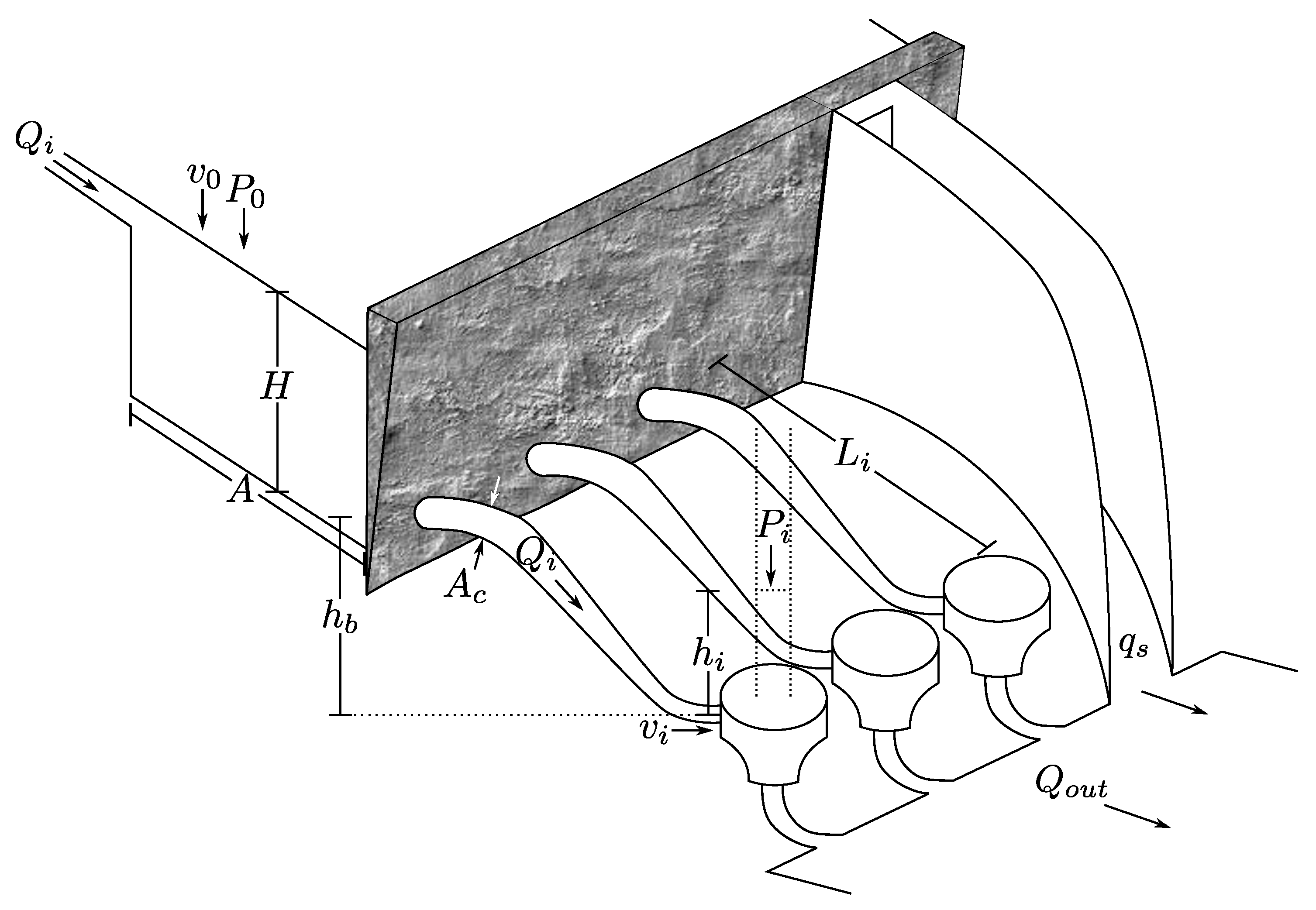
where, $\mathsf{\Delta }P=P_i-P_0$ is the pressure difference, with $P_i$ as the pressure in the turbine i and $P_0$ the atmospheric pressure. $\mathsf{\Delta }H=H+h_b-h_i$ is the difference between the hydraulic head and the turbine level, with $h_b$ as the level from the turbine under the reservoir. The Figure 1 shows the considered architecture. Also, $\mathsf{\Delta }{v}^2=v_0^2-v_i^2$ is the difference between the square of the top and turbine flow velocities. The velocity at the top is assuming $v_0\approx 0$.

Figure 1. Reservoir construction.

The pressure in each turbine is represented as a water column of $h_i$ length, this is $P_i=P_0+h_i\rho g$. Then, from (4), we can see that

$$h_i=\frac{1}{2g}{\left(\frac{Q_i}{A_c}\right)}^2-(H+h_b).$$

(5)

To apply the Inverse Optimal Control algorithm, the system (1)–(3) is discretized

$$\begin{array}{ccc}\hfill H(k+1)& =& H\left(k\right)+\frac{1}{A}\left(Q_{in}\left(k\right)-\sum _{i=1}^n{Q}_i\left(k\right)-q_s\left(k\right)\right)\hfill \end{array}$$

(6)

$$\begin{array}{ccc}\hfill \sum _{i=1}^n{Q}_i(k+1)& =& \sum _{i=1}^n{Q}_i\left(k\right)+\frac{A_{c}g}{L_i}(H\left(k\right)-h_b-h_i\left(k\right))\hfill \end{array}$$

(7)

where, the head at the turbine i is

$$h_i\left(k\right)=\frac{1}{2g}{\left(\frac{Q_i\left(k\right)}{A_c{G}_i\left(k\right)}\right)}^2-(H\left(k\right)+h_b),$$

(8)

being $G_i\left(k\right)$ the i-th gate opening percentage. Finally, the turbines mechanical power generated is computed as follows [8]

$$P_m=\eta g\rho \sum _{i=1}^n{Q}_i\left(k\right)(H\left(k\right)+h_b).$$

(9)

Once the model is presented, first, the algorithm to control the plant is described, and then to this application case is designed.

3. Inverse Optimal Control

Inverse optimal control is a technique, which consists in designing a stabilizing feedback control law, which is based on an a priori known Control Lyapunov Function (CLF), that ensures the optimization of a cost functional [15].

Considering the affine in the control input of a discrete-time nonlinear system

$$\begin{array}{ccc}\hfill x(k+1)& =& f\left(x\right(k\left)\right)+g\left(x\right(k\left)\right)u\left(k\right)\hfill \\ \hfill y\left(k\right)& =& h\left(x\right(k\left)\right)+j\left(x\right(k\left)\right)u\left(k\right)\hfill \end{array}$$

(10)

where $x_0=x\left(0\right)$ and $x\left(k\right)\in {\mathbb{R}}^n$ is the state of the system at time k, the output $y\left(k\right)\in {\mathbb{R}}^m$. Also, the mappings $h:{\mathbb{R}}^n\to {\mathbb{R}}^m$, and $j:{\mathbb{R}}^n\to {\mathbb{R}}^{m\times m}$ are smooth. Under assumption $h\left(0\right)=0$.

To establish the target system, lets consider the following definition

Definition 1

(Passivity). The dynamic system (10) is said to be passive for a supply rate $w\left(y\right(k),$$u\left(k\right))=y^T\left(k\right)u\left(k\right)$ if there exists a non–negative function $S\left(x\right(k\left)\right)$ with $S\left(0\right)=0$, defined as the storage function, such that for all $u\left(k\right)$

$$S\left(x(k+1)\right)-S\left(x\left(k\right)\right)\le y_k^{T}u\left(k\right)$$

(11)

which is named the passivation inequality [14].

For passive systems, asymptotic stability can be achieved using the output feedback

$$u\left(k\right)=-y\left(k\right),$$

setting the storage function $S\left(x\right(k\left)\right)>0$ as a Lyapunov function $\mathcal{V}\left(x\right(k\left)\right)$.

On the other hand, a purpose of this control scheme is to make (10) to a passivated system through the feedback input, this system is defined as follows

Definition 2

(Feedback Passive System). The system (10) is said to be Feedback Passive if there exists a passivation law

$$u\left(k\right)=\alpha \left(x\right(k\left)\right)+v\left(k\right),$$

(12)

with $v\left(k\right)\in {\mathbb{R}}^m$ as the new input and α is a smooth function of the suitable dimension. Such that, the CLS (10), (12) is described by

$$\begin{array}{ccc}\hfill x(k+1)& =& \overline{f}\left(x\left(k\right)\right)+g\left(x\left(k\right)\right)v\left(k\right)\hfill \\ \hfill \overline{y}\left(k\right)& =& \overline{h}\left(x\left(k\right)\right)+\overline{j}\left(x\left(k\right)\right)v\left(k\right),\hfill \end{array}$$

(13)

where $\overline{f}\left(x\left(k\right)\right)=f\left(x\left(k\right)\right)+g\left(x\left(k\right)\right)\alpha \left(x\left(k\right)\right)$ and $\overline{h}$ a smooth mapping with $\overline{h}\left(0\right)=0$. Satisfies the relation

$$\mathcal{V}\left(x(k+1)\right)-\mathcal{V}\left(x\left(k\right)\right)\le \overline{y}{\left(k\right)}^{T}v\left(k\right).$$

The Inverse Optimal Control is formulated as follows: consider the passivity condition $\mathcal{V}\left(x(k+1)\right)-\mathcal{V}\left(x\left(k\right)\right)\le \overline{y}{\left(k\right)}^{T}v\left(k\right)$ with a candidate Lyapunov function

$$\mathcal{V}\left(x\left(k\right)\right)=\frac{1}{2}x{\left(k\right)}^{T}Px\left(k\right),$$

(14)

where $P=P^T>0$. And the control input as in (12), where the passifying law is

$$\begin{array}{ccc}\hfill \alpha \left(x\right(k\left)\right)& =& -{(I_m+\overline{j}\left(x\left(k\right)\right))}^{-1}\overline{h}\left(x\left(k\right)\right)\hfill \\ \hfill v\left(k\right)& =& -\overline{y}\left(k\right),\hfill \end{array}$$

where $I_m$ is the identity matrix, and

$$\begin{array}{ccc}\hfill \overline{h}\left(x\left(k\right)\right)& =& g^T\left(x\left(k\right)\right)P\overline{f}\left(x\left(k\right)\right)\hfill \\ \hfill \overline{j}\left(x\left(k\right)\right)& =& \frac{1}{2}{g}^T\left(x\left(k\right)\right)Pg\left(x\left(k\right)\right).\hfill \end{array}$$

(15)

If there exists P such that

$$\overline{f}{\left(x\left(k\right)\right)}^{T}P\overline{f}\left(x\left(k\right)\right)-x{\left(k\right)}^{T}Px\left(k\right)\le 0,$$

then, the system (10) with input (12) is globally asymptotically stable at the equilibrium point $x\left(k\right)=0$. Moreover, is inverse optimal in the sense that the input control minimizes the meaningful functional given by [16]

$$\mathcal{J}\left(x\left(k\right)\right)=\sum _{k=0}^{\infty }\mathcal{L}(x\left(k\right),\alpha \left(x\left(k\right)\right))$$

where $\mathcal{L}(x\left(k\right),\alpha \left(x\left(k\right)\right))=l\left(x\left(k\right)\right)+{\alpha }^T\left(x\left(k\right)\right)\alpha \left(x\left(k\right)\right)$, $l\left(x\left(k\right)\right)=-\frac{1}{2}(\overline{f}{\left(x\left(k\right)\right)}^{T}P\overline{f}\left(x\left(k\right)\right)-x{\left(k\right)}^{T}Px\left(k\right))\le 0$ and the optimal function value is ${\mathcal{J}}^{*}\left(x\left(0\right)\right)=\mathcal{V}\left(x\left(0\right)\right)$.

For this application, two inverse optimal control schemes are applied. First, to tracking a level reference from the hydraulic head using the spillway as a control input, and then to tracking a mechanical power using the gates to manipulate the flow rate for each turbine.

To apply the desired algorithm, it is necessary to know the discrete model on its totality (6)–(7); in particular, for the hydraulic level, it is necessary to know the flow rate $Q_{in}\left(k\right)$ occurring at every day. With this in mind, a NN is proposed to predict the flow rate. The proposed general scheme is shown in Figure 2. Once the flow rate occurring during the day is predicted, the IOC is applied to the continuous plant model by knowing the level and flow rate references.

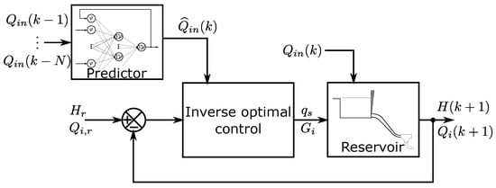
Figure 2. Control–forecasting scheme to reservoir.

It is supposed that A, $A_c$, $L_i$, and $h_b$ are all known, although this may have slight measurement variations with regard to their real dimensions, this under the supposition that, in case of a landslide, some of their magnitudes may become altered. To compensate for these deviations, an error cumulative action is proposed for each of the outputs that are required to be controlled.

$$\begin{array}{ccc}\hfill i_H(k+1)& =& i_H\left(k\right)+H\left(k\right)-H_r\left(k\right)\hfill \end{array}$$

(16)

$$\begin{array}{ccc}\hfill i_Q(k+1)& =& i_Q\left(k\right)+Q_i\left(k\right)-Q_{i,r}\left(k\right),\hfill \end{array}$$

(17)

where $H_r\left(k\right)$ and $Q_{i,r}\left(k\right)$ are the hydraulic head and flow rate references, respectively. Also, $i_H\left(k\right)$ is the level error accumulation and $i_Q\left(k\right)$ is the flow rate error accumulation. These magnitudes correspond to the discretization of integral action for continuous systems [18].

Then, for the hydraulic head subsystem (6)–(16), the estimation of input flow rate ${\widehat{Q}}_{in}\left(k\right)$, and the reference $H_r\left(k\right)$ are assume knowing. To control $q_s$, this estimation is adding, then, the control law results

$$q_s\left(k\right)=-\frac{1}{2}{(I+{\overline{j}}_H\left(k\right))}^{-1}{\overline{h}}_H\left(k\right)-v_H\left(k\right)+{\widehat{Q}}_{in}\left(k\right),$$

(18)

where

$$\begin{array}{ccc}\hfill {\overline{j}}_H& =& {\overline{g}}_H^T{P}_H{\overline{g}}_H\hfill \end{array}$$

(19)

$$\begin{array}{ccc}\hfill {\overline{h}}_H\left(k\right)& =& {\overline{g}}_H^T{P}_H{\overline{f}}_{e,H}\left(k\right)\hfill \\ \hfill {\overline{g}}_H& =& \left[\begin{array}{c}-1/A\\ 0\end{array}\right]\hfill \\ \hfill {\overline{f}}_{e,H}\left(k\right)& =& {\overline{f}}_H\left(k\right)-\left[\begin{array}{c}{H}_r\left(k\right)\\ 0\end{array}\right]\hfill \\ \hfill {\overline{f}}_H\left(k\right)& =& \left[\begin{array}{c}-\sum Q_i\left(k\right)/A\\ i_H\left(k\right)+H\left(k\right)-H_r\left(k\right)\end{array}\right],\hfill \end{array}$$

(20)

the matrix $P_H$ is found through PSO algorithm. Finally, as a new control input to the passivated subsystem is choose

$$v_H\left(k\right)=\left[10.1\right]\left[\begin{array}{c}H\left(k\right)-H_r\left(k\right)\\ i_H\left(k\right)\end{array}\right],$$

since the subsystem output is defined as a linear combination of the tracking error and the error accumulation.

In the case of the mechanical power, by knowing the reference $P_r\left(k\right)$, we calculate $Q_{i,r}\left(k\right)$ from $H\left(k\right)$ using (9) by imposing the same flow circulation in all turbines, this is $Q_{i,r}=Q_{i+1,r}$ for $i=\{1,2,\dots ,n-1\}$. Thus, with a known $Q_{i,r}$, we use $h_i\left(k\right)$ as a pseudo–controller to calculate the opening of each gate $G_i$ using (8). Thus, the Inverse Optimal Controller used for tracking the reference in subsystem (7)–(17) is

$$h_i\left(k\right)=-\frac{1}{2}{(I+{\overline{j}}_Q\left(k\right))}^{-1}{\overline{h}}_Q\left(k\right)+v_Q\left(k\right),$$

(21)

where

$$\begin{array}{ccc}\hfill {\overline{j}}_Q\left(k\right)& =& {\overline{g}}_Q^T\left(k\right)P_Q{\overline{g}}_Q\left(k\right)\hfill \end{array}$$

(22)

$$\begin{array}{ccc}\hfill {\overline{h}}_Q\left(k\right)& =& {\overline{g}}_Q^T\left(k\right)P_Q{\overline{f}}_{e,Q}\left(k\right)\hfill \\ \hfill {\overline{g}}_Q\left(k\right)& =& \left[\begin{array}{c}{A}_c/L_{i}g(H\left(k\right)+h_b-{(Q_i\left(k\right)/A_c)}^2)\\ 0\end{array}\right]\hfill \\ \hfill {\overline{f}}_{e,Q}\left(k\right)& =& {\overline{f}}_Q\left(k\right)-\left[\begin{array}{c}{Q}_{i,r}\left(k\right)\\ 0\end{array}\right]\hfill \\ \hfill {\overline{f}}_Q\left(k\right)& =& \left[\begin{array}{c}{Q}_i\left(k\right)\\ i_Q\left(k\right)+Q_i\left(k\right)-Q_{i,r}\left(k\right)\end{array}\right].\hfill \end{array}$$

(23)

Matrix $P_Q$ is found using the PSO algorithm [32]. Also, the new input for the control of this passive subsystem is

$$v_Q\left(k\right)=\left[10.1\right]\left[\begin{array}{c}{Q}_i\left(k\right)-Q_{i,r}\left(k\right)\\ i_Q\left(k\right)\end{array}\right].$$

Thus, from (8), using head at the turbine as in (21) we get the control law for the opening

$$G_i=\sqrt{\left|\frac{Q_i^2\left(k\right)}{2g(h_i\left(k\right)+H\left(k\right)+h_b)A_c^2}\right|}.$$

(24)

which represent the opening rate $G_i\in (0,1]$, on each gate so that the pressure on each turbine i correspond to a water column $h_i$ in meters.

To find the matrix $P_H$ and $P_Q$, we used the PSO algorithm describe in follows.

Metaheuristic Algorithm

The Particle Swarm Optimization (PSO) algorithm [33] is used in the IOC procedure to find the matrix that guarantees asymptotic stability in passivity CL–system [15,16,17,21].

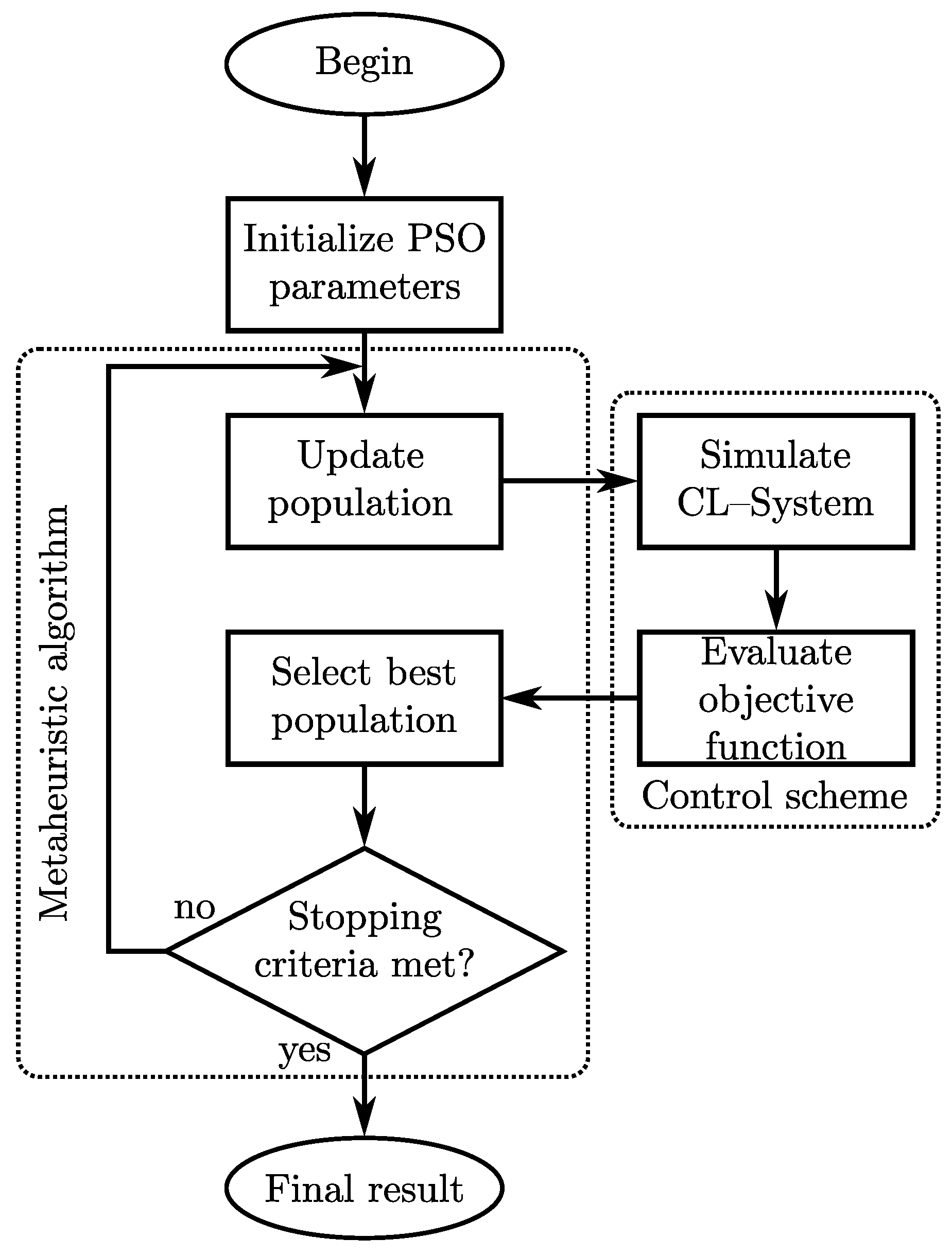
The algorithm describes the social behavior of birds and fish. It relies mostly on the basic principles of self–organization. The algorithm starts with a population of random position, the control scheme in Figure 2 is evaluated under a minimization criterion J, the best positions are selected from the proposed criterion. Then, the positions and velocities of the particles are recalculated so that the objective function decreases, this process is repeated until a stopping criterion is met. The flowchart is depicted in Figure 3.

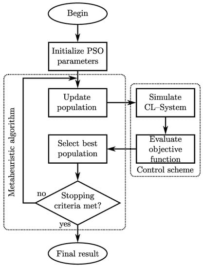
Figure 3. PSO algorithm flowchart.

To update the population, the follow equations are presented

$$\begin{array}{ccc}\hfill V_i(t+1)& =& w\left(t\right)V_i\left(t\right)+r_1{c}_1(L_i\left(t\right)-K_i\left(t\right))+r_2{c}_2(B\left(t\right)-K_i\left(t\right))\hfill \\ \hfill K_i(t+1)& =& K_i\left(t\right)+V_i(t+1)\hfill \end{array}$$

(25)

where $V_i\left(t\right)$ is the velocity of particle i at time t, $K_i\left(t\right)$ is the position of particle. The first element in velocity equation is the inertia term, next the cognitive component, and finally, the social component. Besides, $w\left(t\right)$ is the inertia coefficient, $c_1$ and $c_2$ are the personal and social acceleration coefficient, respectively. $r_1$ and $r_2$ are two uniformly aleatory numbers between $(0,1]$. $L_i\left(t\right)$ is the personal best position of particle i, and $B\left(t\right)$ is the social best position.

Additionally, the inertia coefficient is damping in each iteration by.

$$w(t+1)=w\left(t\right)w_{damp}.$$

Then, the matrix $P_H$ and $P_Q$ used in (19), (20), (22), and (23) are constructed from B at final iteration as follows

$$\begin{array}{ccc}\hfill P_H& =& \left[\begin{array}{cc}{b}_1& b_2\\ b_2& b_3\end{array}\right]\hfill \\ \hfill P_Q& =& \left[\begin{array}{cc}{b}_4& b_5\\ b_5& b_6\end{array}\right],\hfill \end{array}$$

being, $b_i$, with $i=\{1,2,\dots ,6\}$, the elements of $B=[b_1,b_2,\dots ,b_6]$. From that, the dimension of each particle is six.

4. Forecasting

The inverse optimal control algorithm by itself is not robust [17], since it is limited to the fact that, through an inverse model, the system behaves passively, to later stabilize it. For this reason, an integral gain is added to each output to attenuate the parametric variations of the system, however, in the presence of external disturbance, such as $Q_{in}$, the results may not be as expected.

To reduce the effect of flow velocity at the input, a NN is designed. this NN is based on the nature of the historical data. To obtain a better representation of the signal, a series of treatments are applied to reduce the possible effect of noise on sensors, human error, or data loss. Treatment is as follows:

• Missing values imputation using Nearest Neighbor method [26].
• Discrete low–pass filtering [27,28].
• Yeo–Johnson transformation to minimize variance in prediction [31].
• Identification and imputation of atypical data by the quantile method [29].
• Offset and scaling [30].

When obtaining a prediction, the inverse of scaling and offset must be applied to the result.

Once we have our pre-processed data is obtained, we construct the NN by taking the following criteria into account:

• The signal auto-correlation.

  Hypothesis 1.

  The auto-correlation indicates the number of sufficient inputs of previous data that have less relation with each other. In this way it does not fall into information redundancies.
• Order estimation of the system that generates the signal.

  Hypothesis 2.

  If the signal is a solution of a differential equation of order n, then, $n-1$ feedback outputs are sufficient.
• Signal frequency.

  Hypothesis 3.

  The number of hidden layers in the NN is directly proportional to the frequencies of the signal to be represented.
• Finally, the number of data to be predicted is considered, which is the number of outputs of the mentioned network.

These hypotheses are proposed and applied in this work but we plan to develop them in-depth as the main contribution in a future work.

To calculate the auto-correlation, we define a set of elements that constitute the signal as

$$s(a,b)=\{Q_{in}\left(a\right),Q_{in}(a+1),\dots ,Q_{in}\left(b\right)\},$$

with $0<a<b$. Then, the auto–correlation using the x previous elements is calculated as follows:

$$C\left(x\right)=\underset{x<k<size\left(Q_{in}\right)-1}{min}\frac{\sum (s(k-x,k)-{\mu }_x)(s(k-x,k+1)-\mu )}{x{\sigma }_x\sigma },$$

where, ${\mu }_x$ and ${\sigma }_x$ are the mean and standard deviation for $s(k-x,k)$, whereas $\mu$ and $\sigma$ stand for the mean and standard deviation for $s(k-x,k+1)$.

5. Simulation

5.1. Tracking Control

Let’s take the Inverse Optimal Control scheme shown in Figure 2. As reference, we use the hydraulic head and mechanical power described by the following equation

$$\begin{array}{ccc}\hfill H_r& =& 60+5cos\left(0.05t\right)\hfill \\ \hfill P_{m,r}& =& 0.8g\left(60+5cos\left(0.05t\right)\right)\left(1300+100sin\left(0.2t\right)sin(t/365)\right).\hfill \end{array}$$

If the hydraulic system has three turbines, and the control reference for each flow is known, for an efficiency of $\eta =0.8$, we have that:

$$Q_{i,r}=\frac{1300}{3}+\frac{100}{3}sin\left(0.2t\right)sin(t/365).$$

Assuming a trained NN, the control gains are found through the PSO algorithm. The stopping criteria is to reach 100 iterations. The objective function is

$$J=\frac{J_Q(T_{1,Q}+T_{2,Q})}{{\sum }_{k=1}^{T_{1,Q}+T_{2,Q}}{Q}_{i,r}^2\left(k\right)}+\frac{J_H(T_{1,H}+T_{2,H})}{{\sum }_{k=1}^{T_{1,H}+T_{2,H}}{H}_r^2\left(k\right)},$$

(26)

where $T_{1,Q}$ and $T_{2,Q}$ are the transitory and stationary time for the flow rate. $T_{1,H}$ and $T_{2,H}$ are the times analog to flow rate for hydraulic head. $J_Q$ and $J_H$ are the objective functions associated to tracking error from flow rate, and hydraulic head, respectively. The corresponds objective function are computed as

$$J_Q=w_{1,Q}\frac{1}{T_{1,Q}}\sum _{k=1}^{T_{1,Q}}{(Q_{i,r}\left(k\right)-Q_i\left(k\right))}^2+w_{2,Q}\frac{1}{T_{2,Q}}\sum _{k=T_{1,Q}+1}^{T_{1,Q}+T_{2,Q}}{(Q_{i,r}\left(k\right)-Q_i\left(k\right))}^2,$$

(27)

being, $w_{1,Q}$ and $w_{2,Q}$ are constants to weigh the transient and steady state for $Q_i$.

On the other hand, the objective function of the hydraulic head is

$$J_H=w_{1,H}\frac{1}{T_{1,H}}\sum _{k=0}^{T_{1,H}}{(H_r\left(k\right)-H\left(k\right))}^2+w_{2,H}\frac{1}{T_{2,H}}\sum _{k=T_{1,H}+1}^{T_{1,H}+T_{2,H}}{(H_r\left(k\right)-H\left(k\right))}^2,$$

(28)

with $w_{1,H}$ and $w_{2,H}$ as constants to weigh the transient and steady state for H.

In other matters, the constants used in (27) and (28) are described in Table 1.

Table 1. Constants used in the objective function.

Constant	Value
$w_{1,Q}$	0.01
$w_{2,Q}$	0.99
$w_{1,H}$	0.01
$w_{2,H}$	0.99
$T_{1,Q}$	2 days
$T_{2,Q}$	3285 days
$T_{1,H}$	20 days
$T_{2,H}$	3267 days

Furthermore, on the PSO algorithm, we use the parameters described in Table 2.

Table 2. Parameters used in PSO algorithm.

Parameter	Description	Value
N	population	500 particles
$c_1$	personal acceleration coefficient	2
$c_2$	social acceleration coefficient	2
w	inertia coefficient	1
$w_{damp}$	damping ratio of inertia coefficient	0.99

Besides, the range search is between $[-1,5000]$. The algorithm is simulated using the code provided by the Yarpiz team [34].

5.2. Inverse Optimal Control including Parametric Variations

Further, at May–2013 a landslide is simulated, this causes an increase in the hydraulic head of 10 m, a decrease of the reservoir area, and obstruction in duct area of $50\%$. It is expected that these parametric changes are attenuated by the cumulative dynamic proposed in this work. The simulated system includes a discrete model of the hydropower plant (6)–(7) and the Inverse Optimal Controller (18)–(24) with cumulative action (16)–(17).

5.3. Inverse Optimal Control including External Disturbances

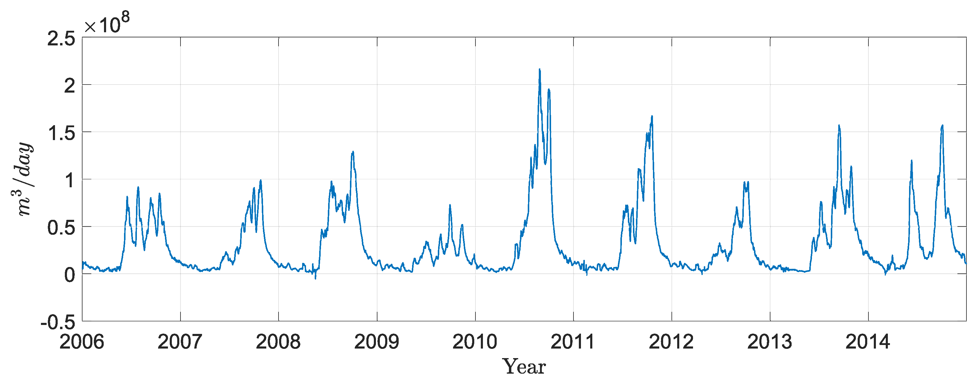
To eliminate the undesired effect of increasing the hydraulic head, knowing the flow that serves as the input of the hydropower system is required. Thus, it is needed to construct a neural predictor to estimate the flow at each day k, to do this, we first process the data needed to train such predictor. The historical data for $Q_{in}$ is shown in the Figure 4 and its attributes are depicted in Table 3. From this table, it may be noticed that the minimum value of the flow is rate negative; however, as the flow rate must be positive, these negative values are considered outliers.

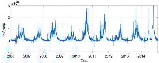
Figure 4. Historical data for $Q_{in}$ without pre–processing.

Table 3. Attributes for historical data $Q_{in}$.

Attribute	Value
count	3202
mean	30.882717
std	39.399464
min	−73.790000
max	299.740000
missed	85

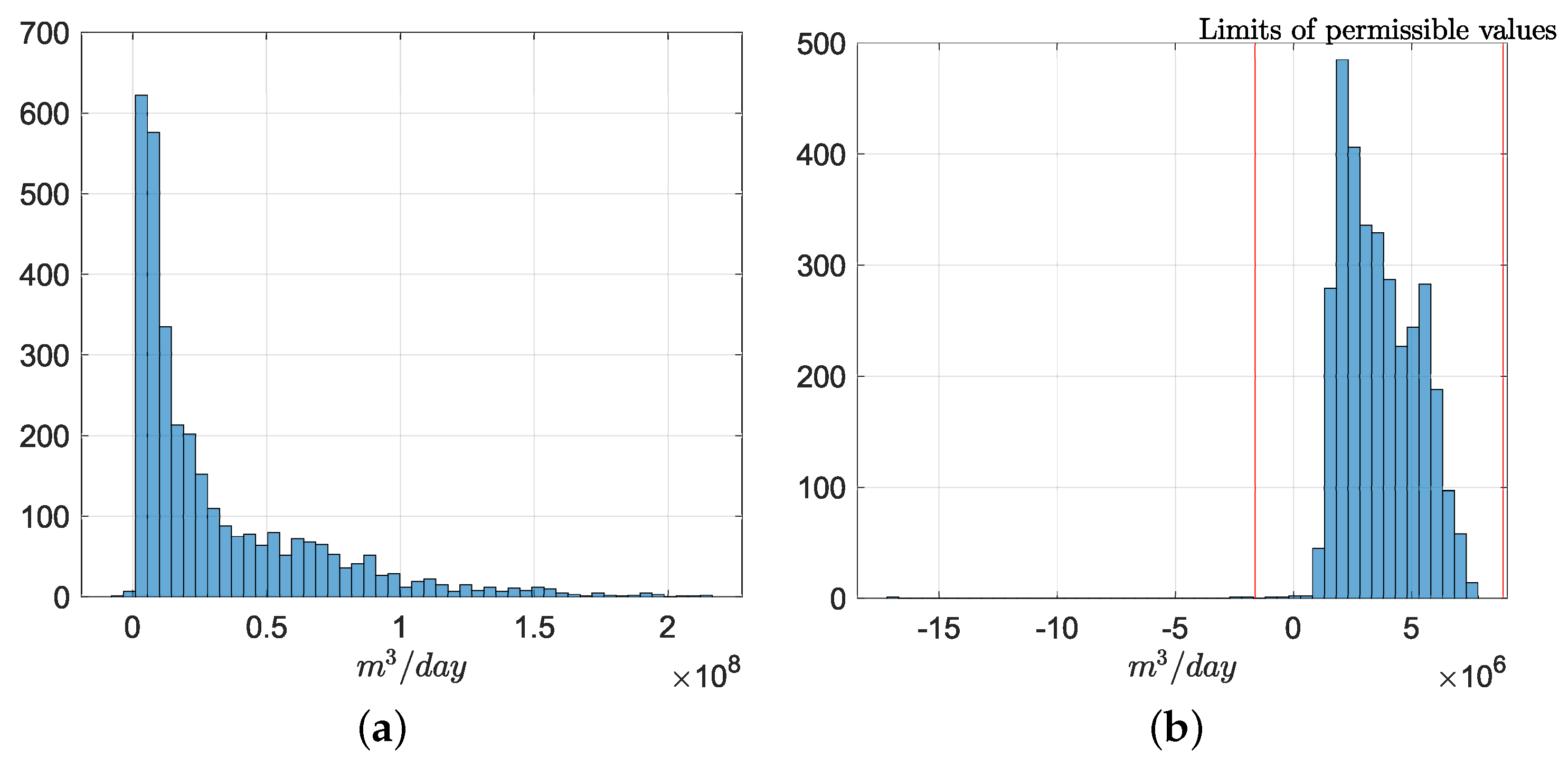
The results of inputting the missing values and applied the discrete low–pass filter, is displayed in Figure 5, after, the data is studied from a frequency point of view, then, a Yeo–Johnson transform is applied to discriminate the outliers values, this is considered all values $1.5(q_3-q_1)$ times under $q_1$ or upper $q_3$, where $q_1$ and $q_3$ are the first and third quartile of the data filtered, respectively. A comparative histogram is shown in Figure 6. The parameter to transform the data is calculated from the maximum likelihood method, this is $\lambda =0.12217$.

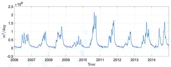
Figure 5. Historical data of $Q_{in}$ filtered with missing values imputed.

Figure 6. Comparative histogram of filtered data and the Yeo–Johnson transform. (a) Filtered data histogram. (b) Transformed data histogram.

Once the obtained data is clean, based on the attributes shown in Table 4, the negative values suggest an offset on the sensor reading of at least $0.7090$. This value must be found by testing the model recursively on the plant. A first compensation value of $0.8000$ is proposed.

Table 4. Attributes of data cleaning.

Attribute	Value
count	3287
mean	31.8105
std	35.8087
min	−0.7090
max	216.3110

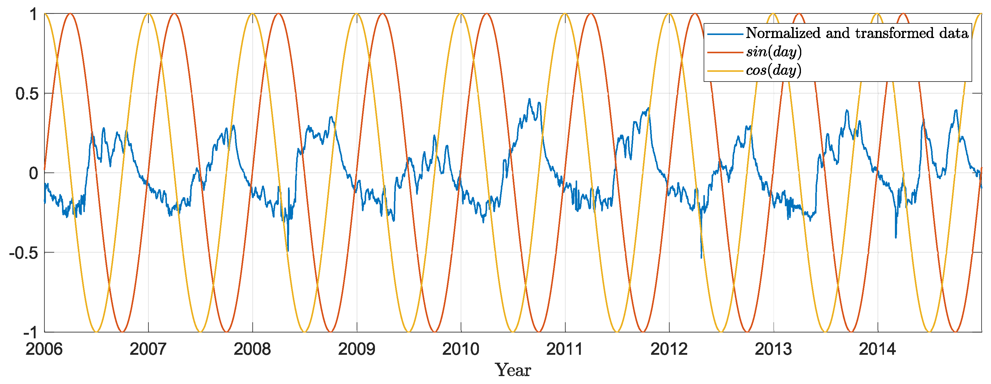
The input for the transformed data is scaled so that its response values are $-1\le x\le 1$ with mean zero, and they are added to time in the form of a sine/cosine signal with a period of one year to the NN input. These inputs are shown in Figure 7.

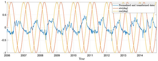
Figure 7. Input data to NN.

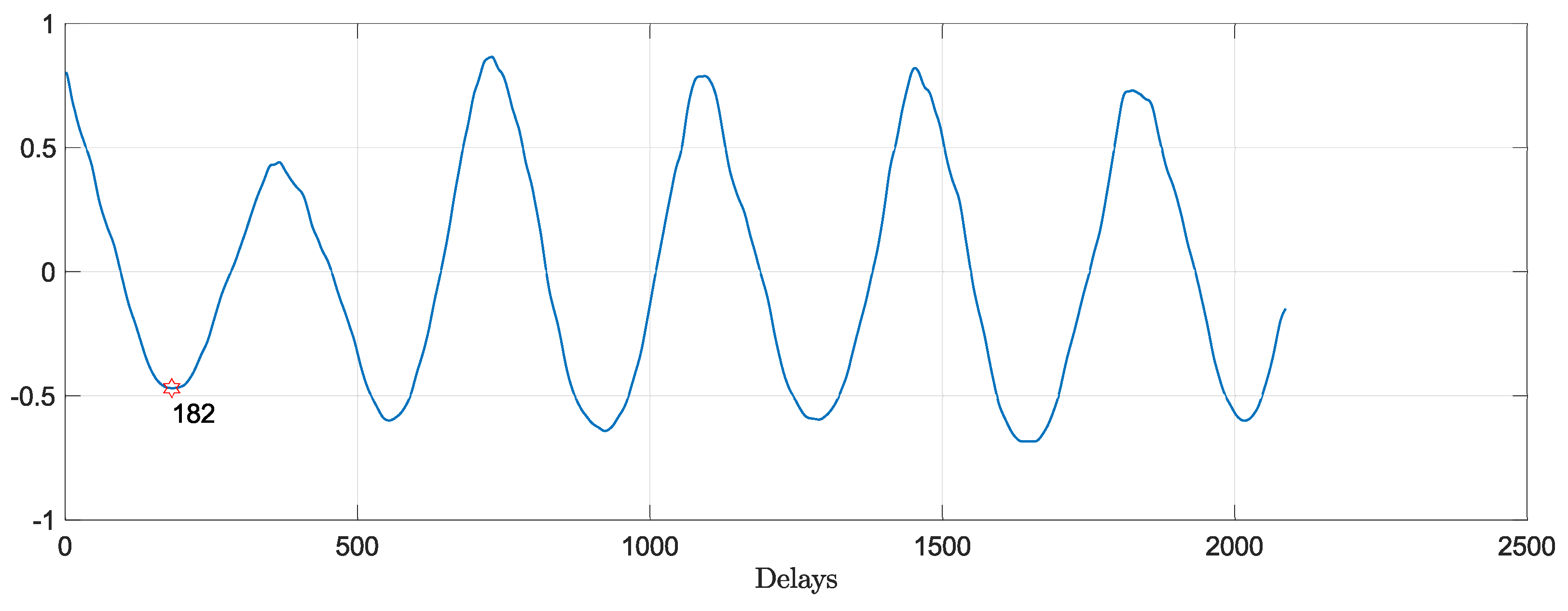
For the design of the NN, we find the auto-correlation of the clean data. In Figure 8 it is shown that with $x=182$ the first minimum is reached, thus this value is chosen as the number of inputs for the previous days.

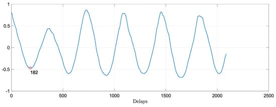
Figure 8. Signal auto-correlation from historical data.

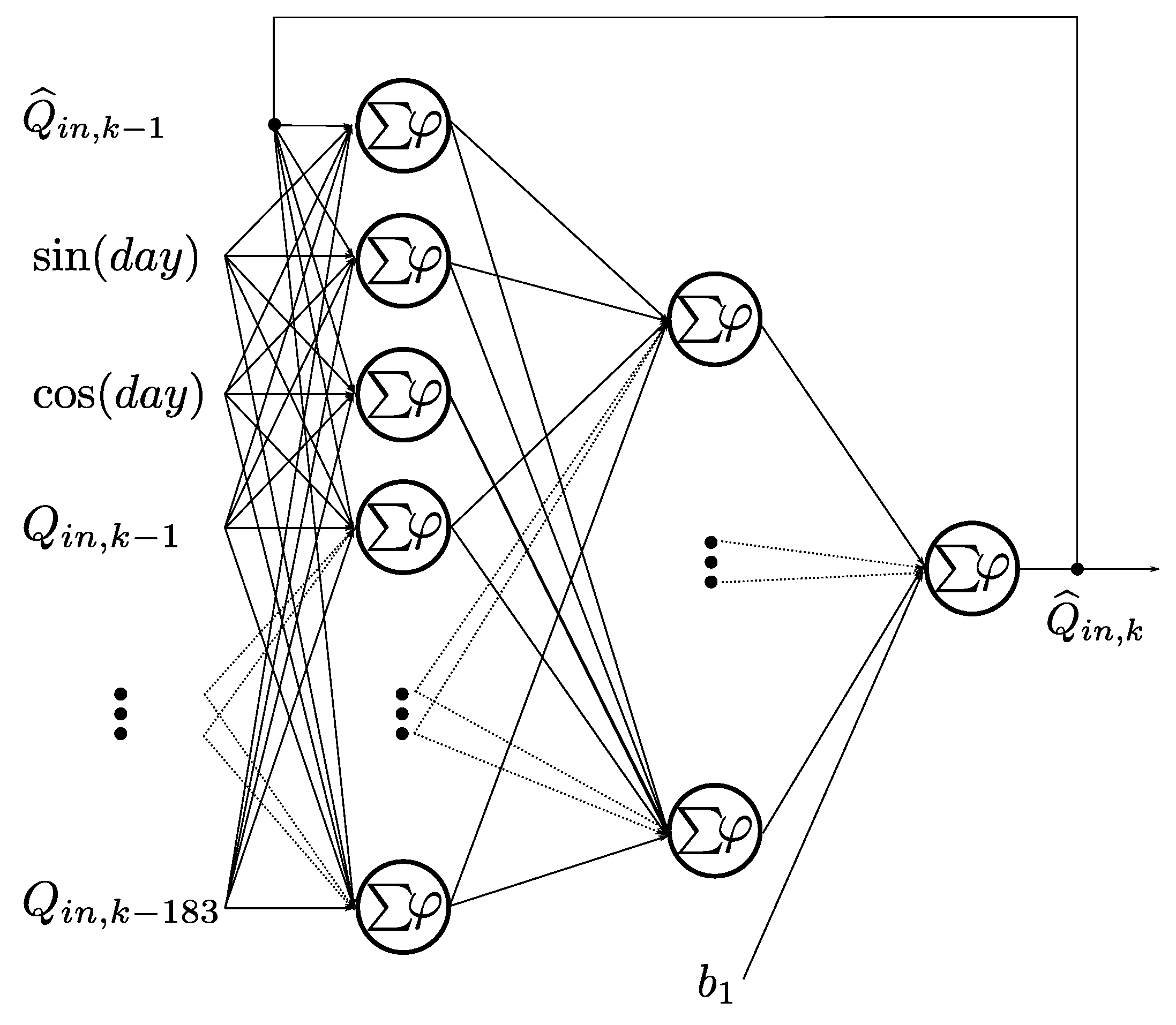
To know the number of output elements yr that are feedback to the NN, we start from the supposition that this signal may be generated by knowing its actual value, as well as its derivative, this supposing a 2nd order system; this means that a delay of the output is enough to feedback, $y_r=1$. Furthermore, it is supposed that, due to its periodicity, the NN only requires a hidden layer to be applied. The number of neurons before the output layer is directly proportional to the desired resolution, thus, it is proposed to use 30 of them. The number of neurons on the input layer is given by $5(x+yr+dt)$, where $dt$ stands for the number of elements considered to model time. The scheme of the applied NN is shown in Figure 9.

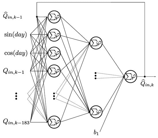
Figure 9. NN to forecasting.

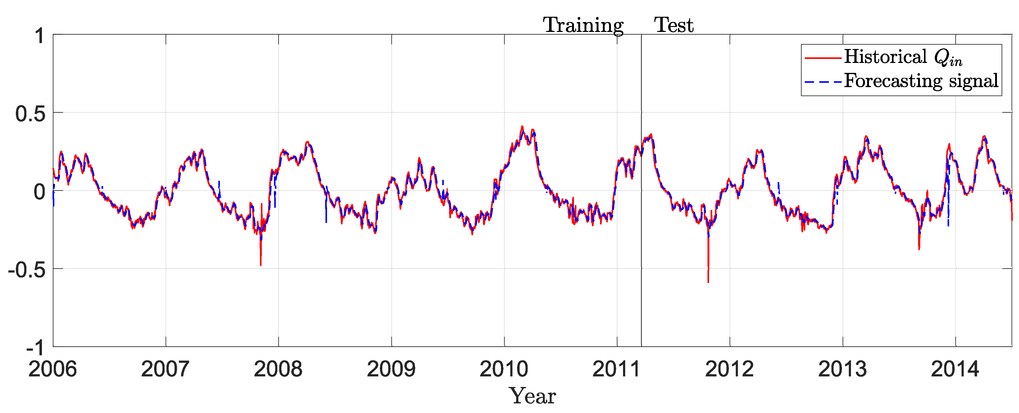
The historical data taken to train the NN contemplates the hydraulic head monitored through January-2006 to April-2011. On the other hand, data from April-2011 to December-2014 is utilized to test the prediction model.

6. Results and Discussions

6.1. Model: Technical Considerations

Due to the control robustness, a non-linear model is described simplifying the losses due to evaporation, friction, leaks, etc. These are absorbed by the cumulative action of the IOC.

The model contemplates that the reservoir must always maintain a minimum level of water. This level has to be greater than the diameter of the cross-section to avoid variations in mass from (2).

The power generated by the turbines is calculated as a stationary state. This is assuming an adequate speed regulation in the governor.

The model includes a spillway as a control input which is used as an alternative to releasing water when the levels of the dam exceed the reference. This work does not contemplate policies of release by spillways that limit the outflow. A general multipurpose study is necessary for the proper management of the water diverted by the system. This analysis should consider the need to satisfy specific demands, such as agriculture, navigation, human accents, among others. To know the destination of the water released by the spillway, as well as the limits of the river to avoid risks and losses in the aforementioned aspects.

6.2. Tracking Control

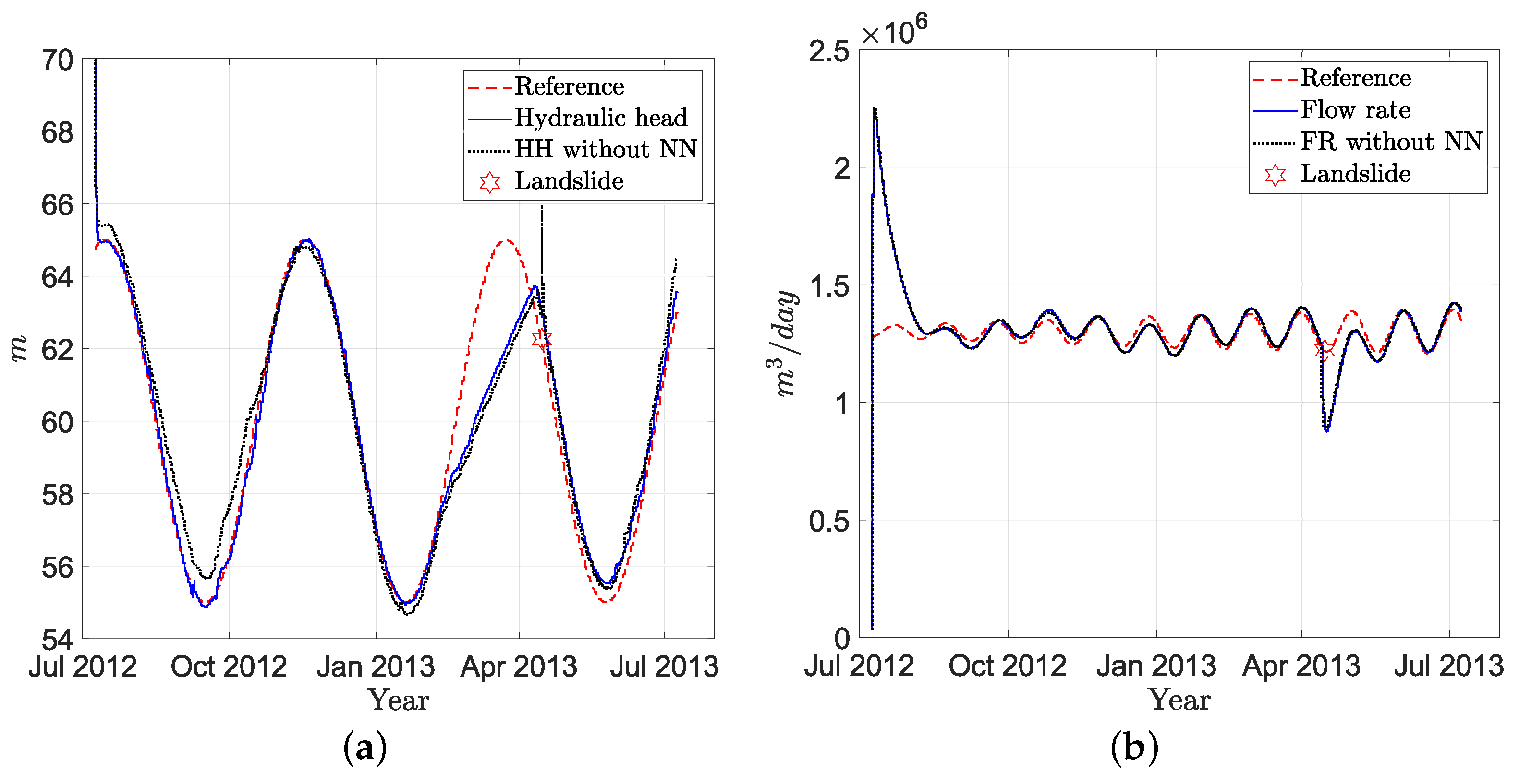
At the end of the metaheuristic algorithm, the best cost was $0.0128$ with position $B=[6.4409,-1.0000,15.7979,50,000.00,21.654,2835.136]$. The Figure 10 shows a comparison between hydraulic head reference and Inverse optimal control output without forecasting (dotted line), Figure 10a. Also, the Figure 10b shows a comparison between the flow rate reference (discontinuous line) and the output without forecasting (dotted line). From this, it is observed that there is a period where the hydraulic head remains below the reference. This is because the permitted limit is greater than that provided by the input flow, which suggests a dry season.

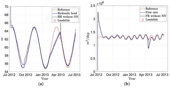
Figure 10. Flow rate and Hydraulic head output comparison. (a) Hydraulic head output and reference. (b) Flow rate output and reference.

6.3. Inverse Optimal Control including Parametric Variations

By simulating the controller without prediction data, we get a root mean squared error of 0.0145. Thanks to the integral action it is possible to handle perturbations $Q_{in}$, however, the hydraulic head is above the permitted limit, which could be undesirable. The landslide is marked with a star in Figure 10. Figure 10a shows a comparison between hydraulic head references and IOC output with accumulative action (dotted line). Furthermore, Figure 10b shows a comparison between the flow rate reference (dashed line) and the output (dotted line). It is observed that the controller manages to adjust the response of the system to the desired reference. A prediction block is included to improve this response.

6.4. Inverse Optimal Control including External Disturbances

The response of the applied NN is shown in Figure 11. Data suggest that the filtering criterion is very conservative. There is a presence of values that provoke an unlikely derivative in the signal (this by considering a Bayesian criterion); however, these values are not eliminated with the noise filtering. These results motivate the use of a filter that limits the derivative, which can also update itself as time progress.

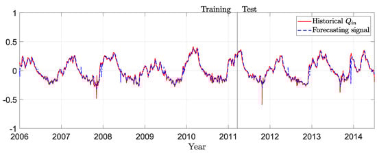
Figure 11. Forecasting to normalized data.

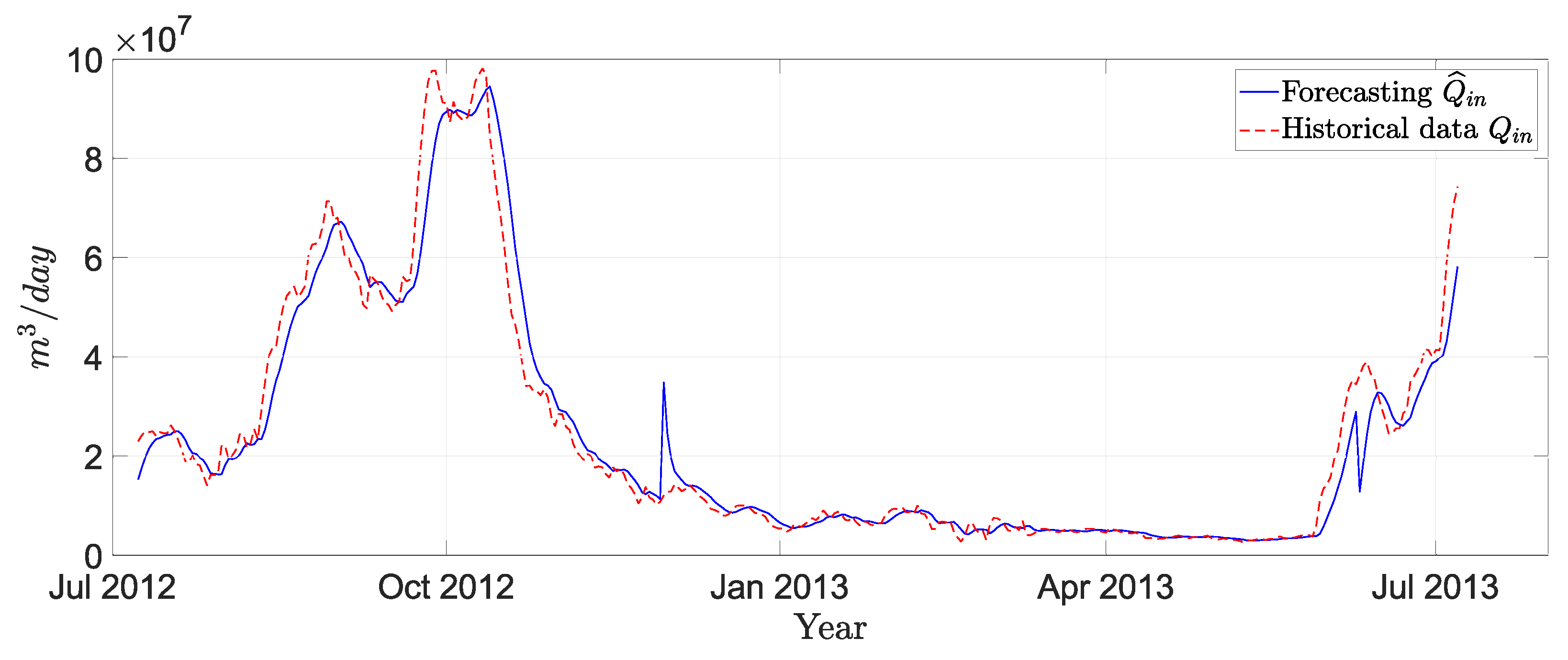
We simulated the operation process of the dam by using the flow rate historical data corresponding to 365 days of operation, starting from July 2012. The resulting prediction outputted by the NN (Figure 9) is used to calculate the inverse Yeo–Johnson function, giving as a result what is shown in Figure 12. However, after discarding and replacing the spurious data with the Yeo–Johnson data transformation (Figure 6) it is possible that the resulting signal has a distribution when said transformation is applied once more. In future works, it is planned to explore the idea of a recursive data transformation–elimination process to minimize spurious data.

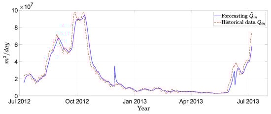
Figure 12. Simulation forecasting to ${\widehat{Q}}_{in}$.

With the inclusion of the NN for prediction we achieve a root mean squared error of 0.0143. The Figure 10a shows a comparison between hydraulic head reference and Inverse Optimal Control output with forecasting (continuous line), Figure 10a. Also, the Figure 10b shows a comparison between the flow rate reference (dashed line) and the IOC output using forecasting (continuous line). The landslide is also simulated in May-2013, causing the same variations of 50%. The control response is depicted in Figure 13, the evolution of $q_s\left(k\right)$ is in Figure 13a and the gate of a turbine is shown in Figure 13b.

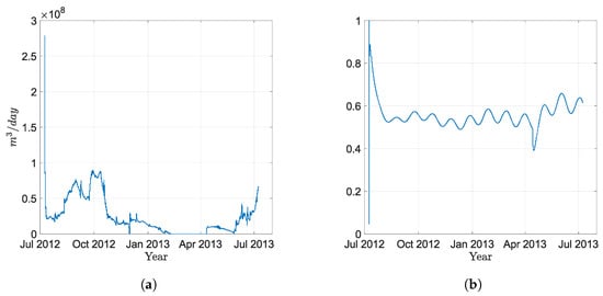
Figure 13. Control inputs using Forecasting NN. (a) Control signal $q_{vert}$. (b) Control signal of a turbine gate.

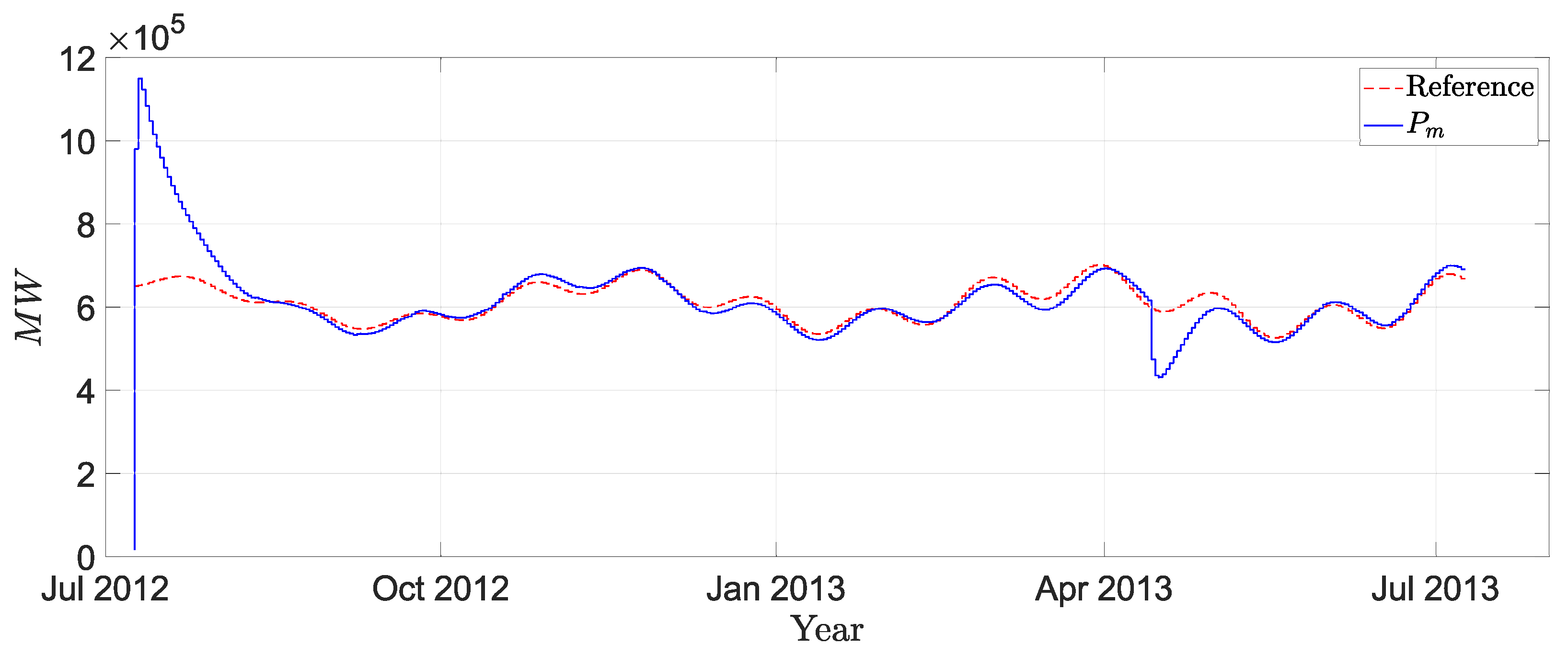
The power generates is shown in Figure 14, where it is compared with the reference signal (dashed line).

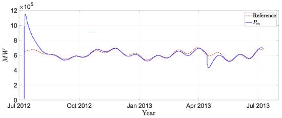
Figure 14. Mechanical Power generation $P_m$.

In here, there are two important observations

• The output in the hydraulic head should always be below the reference since it is considered that the controller input $q_s$ is always positive; this is, the flow is always unidirectional, Figure 10.
• Besides handling parametric variations (such as the case of landslides), the proposed Integral Action Inverse Optimal Controller scheme is also able to properly manage external perturbations; in fact, it is observed that the output of the controller does not differ significantly from the reference, Figure 10.

7. Conclusions

7.1. Tracking Control

The implementation of the Inverse Optimal Control technique for tracking along with the application of the PSO algorithm, the model manages to minimize the tracking error, thus demonstrating it to be a good alternative for adjusting to a time-varying reference. It is been observed that, when modeling a system with abundant flows, a negligible margin of error of up to 1.7% is observed. Following the recommendation proposed in the discussion, it is suggested to establish upper/lower reference limits that allow one to keep the head level below the reference, this is a safety measure.

7.2. Inverse Optimal Control including Parametric Variations

In the event of an unforeseen event (such as a landslide), it is been shown that the Inverse Optimal Control scheme is capable of following the reference with a minimum deviation, thus ensuring that the systems level is maintained close to the reference while also warranting a supply which satisfies the current energy demand despite a reduction in its storage capacity.

7.3. Inverse Optimal Control including External Disturbances

By applying Feature Engineering techniques to the system’s historical data and subsequently feeding the neural network with this information, an excellent approximation is achieved in the training stage and a minimum error in the predictions.

References

- Win, S.; Zin, W.W.; Kawasaki, A.; San, Z.M.L.T. Establishment of flood damage function models: A case study in the Bago River Basin, Myanmar. Int. J. Disaster Risk Reduct. 2018, 28, 688–700. [Google Scholar] [CrossRef]
- Sidle, R.C.; Greco, R.; Bogaard, T. Overview of landslide hydrology. Water 2019, 11, 148. [Google Scholar] [CrossRef] [Green Version]
- Morcillo, J.D.; Angulo, F.; Franco, C.J. Analyzing the hydroelectricity variability on power markets from a system dynamics and dynamic systems perspective: Seasonality and ENSO phenomenon. Energies 2020, 13, 2381. [Google Scholar] [CrossRef]
- Chanson, H. (Ed.) 2-Fundamentals of open channel flows. In Environmental Hydraulics of Open Channel Flows; Butterworth-Heinemann: Oxford, UK, 2004; pp. 11–34. [Google Scholar]
- Mahmoud, M.; Dutton, K.; Denman, M. Dynamical modelling and simulation of a cascaded reserevoirs hydropower plant. Electr. Power Syst. Res. 2004, 70, 129–139. [Google Scholar] [CrossRef]
- Robert, G.; Michaud, F. Hydro power plant modeling for generation control applications. In Proceedings of the 2012 American Control Conference (ACC), Montreal, QB, Canada, 27–29 June 2012; pp. 2289–2294. [Google Scholar]
- Moglen, G.E. Fundamentals of Open Channel Flow; CRC Press: Boca Raton, FL, USA, 2015. [Google Scholar]
- Blair, T.H. Energy Production Systems Engineering; John Wiley & Sons: Hoboken, NJ, USA, 2016. [Google Scholar]
- Huang, S.; Linyun, X.; Wang, J.; Li, P.; Wang, Z.; Ma, M. Fixed-time synergetic controller for stabilization of hydraulic turbine regulating system. Renew. Energy 2020, 157, 1233–1242. [Google Scholar] [CrossRef]
- Reigstad, T.I.; Uhlen, K. Variable speed hydropower conversion and control. IEEE Trans. Energy Convers. 2019, 35, 386–393. [Google Scholar] [CrossRef]
- Gil-González, W.J.; Garces, A.; Fosso, O.B.; Escobar-Mejía, A. Passivity-based control of power systems considering hydro-turbine with surge tank. IEEE Trans. Power Syst. 2019, 35, 2002–2011. [Google Scholar] [CrossRef]
- Sahin, E. Design of an Optimized Fractional High Order Differential Feedback Controller for Load Frequency Control of a Multi-Area Multi-Source Power System with Nonlinearity. IEEE Access 2020, 8, 12327–12342. [Google Scholar] [CrossRef]
- Singh, A.; Ghosh, S. Heuristic Optimization based Controller Design for Voltage Regulation in Small Hydropower Plant. In Proceedings of the 2020 First International Conference on Power, Control and Computing Technologies (ICPC2T), Raipur, India, 3–5 January 2020; pp. 111–116. [Google Scholar]
- Byrnes, C.; Lin, W. Losslessness, feedback equivalence, and the global stabilization of discrete-time nonlinear systems. IEEE Trans. Autom. Control 1994, 39, 83–98. [Google Scholar] [CrossRef]
- Gurubel, K.J.; Sanchez, E.N.; Coronado-Mendoza, A.; Zuniga-Grajeda, V.; Sulbaran-Rangel, B.; Breton-Deval, L. Inverse optimal neural control via passivity approach for nonlinear anaerobic bioprocesses with biofuels production. Optim. Control Appl. Methods 2019, 40, 848–858. [Google Scholar] [CrossRef]
- Gurubel, K.; Osuna-Enciso, V.; Coronado-Mendoza, A.; Cuevas, E. Optimal control strategy based on neural model of nonlinear systems and evolutionary algorithms for renewable energy production as applied to biofuel generation. J. Renew. Sustain. Energy 2017, 9, 033101. [Google Scholar] [CrossRef]
- Sanchez, E.N.; Ornelas-Tellez, F. Discrete-Time Inverse Optimal Control for Nonlinear Systems; CRC Press: Boca Raton, FL, USA, 2017. [Google Scholar]
- Morari, M. Robust stability of systems with integral control. IEEE Trans. Autom. Control 1985, 30, 574–577. [Google Scholar] [CrossRef] [Green Version]
- Ma, H.; Chen, M.; Wu, Q. Disturbance Observer-Based Inverse Optimal Tracking Control of the Unmanned Aerial Helicopter. In Proceedings of the 2019 IEEE 8th Data Driven Control and Learning Systems Conference (DDCLS), Dali, China, 24–27 May 2019; pp. 448–452. [Google Scholar]
- Min, X.; Li, Y.; Tong, S. Adaptive fuzzy output feedback inverse optimal control for vehicle active suspension systems. Neurocomputing 2020, 403, 257–267. [Google Scholar] [CrossRef]
- Djilali, L.; Sanchez, E.N.; Ornelas-Tellez, F.; Ruz-Hernandez, J.A.; Ricalde, L.J. Real-time neural inverse optimal control for low-voltage rid-through enhancement of double fed induction generator based wind turbines. ISA Trans. 2021, 113, 111–126. [Google Scholar] [CrossRef] [PubMed]
- Yang, S.; Yang, D.; Chen, J.; Zhao, B. Real-time reservoir operation using recurrent neural networks and inflow forecast from a distributed hydrological model. J. Hydrol. 2019, 579, 124229. [Google Scholar] [CrossRef]
- Ogliari, E.; Nespoli, A.; Mussetta, M.; Pretto, S.; Zimbardo, A.; Bonfanti, N.; Aufiero, M. A Hybrid Method for the Run-Of-The-River Hydroelectric Power Plant Energy Forecast: HYPE Hydrological Model and Neural Network. Forecasting 2020, 2, 410–428. [Google Scholar] [CrossRef]
- Benidis, K.; Rangapuram, S.S.; Flunkert, V.; Wang, B.; Maddix, D.; Turkmen, C.; Gasthaus, J.; Bohlke-Schneider, M.; Salinas, D.; Stella, L.; et al. Neural forecasting: Introduction and literature overview. arXiv 2020, arXiv:2004.10240. [Google Scholar]
- Zheng, A.; Casari, A. Feature Engineering for Machine Learning: Principles and Techniques for Data Scientists; O’Reilly Media, Inc.: Sebastopol, CA, USA, 2018. [Google Scholar]
- Tutz, G.; Ramzan, S. Improved methods for the imputation of missing data by nearest neighbor methods. Comput. Stat. Data Anal. 2015, 90, 84–99. [Google Scholar] [CrossRef] [Green Version]
- Smith, S.W. (Ed.) Chapter 15—Moving Average Filters. In Digital Signal Processing; Newnes: Boston, MA, USA, 2003; pp. 277–284. [Google Scholar] [CrossRef]
- Babu, C.N.; Reddy, B.E. A moving-average filter based hybrid ARIMA–ANN model for forecasting time series data. Appl. Soft Comput. 2014, 23, 27–38. [Google Scholar] [CrossRef]
- Wilcox, R. (Ed.) Chapter 3—Estimating Measures of Location and Scale. In Introduction to Robust Estimation and Hypothesis Testing, 4th ed.; Statistical Modeling and Decision Science; Academic Press: Cambridge, MA, USA, 2017; pp. 45–106. [Google Scholar] [CrossRef]
- Kuhn, M.; Johnson, K. Feature Engineering and Selection: A Practical Approach for Predictive Models; CRC Press: Boca Raton, FL, USA, 2019. [Google Scholar]
- Yeo, I.K.; Johnson, R.A. A new family of power transformations to improve normality or symmetry. Biometrika 2000, 87, 954–959. [Google Scholar] [CrossRef]
- Kennedy, J.; Eberhart, R. Particle swarm optimization. In Proceedings of the ICNN’95—International Conference on Neural Networks, Perth, WA, Australia, 27 November–1 December 1995; Volume 4, pp. 1942–1948. [Google Scholar]
- Eberhart, R.; Kennedy, J. A new optimizer using particle swarm theory. In Proceedings of the Sixth International Symposium on Micro Machine and Human Science, Nagoya, Japan, 4–6 October 1995; pp. 39–43. [Google Scholar]
- Yarpiz. Particle Swarm Optimization (PSO) in MATLAB—Video Tutorial. 2016. Available online: https://yarpiz.com/440/ytea101-particle-swarm-optimization-pso-in-matlab-video-tutorial (accessed on 28 June 2021).
Publisher’s Note: MDPI stays neutral with regard to jurisdictional claims in published maps and institutional affiliations. |
© 2021 by the authors. Licensee MDPI, Basel, Switzerland. This article is an open access article distributed under the terms and conditions of the Creative Commons Attribution (CC BY) license (https://creativecommons.org/licenses/by/4.0/).