
Inverse Optimal Control Using Metaheuristics of Hydropower Plant Model via Forecasting Based on the Feature Engineering

 ,
,  ,
,  and
and 
Abstract
:1. Introduction
Contribution and Organization
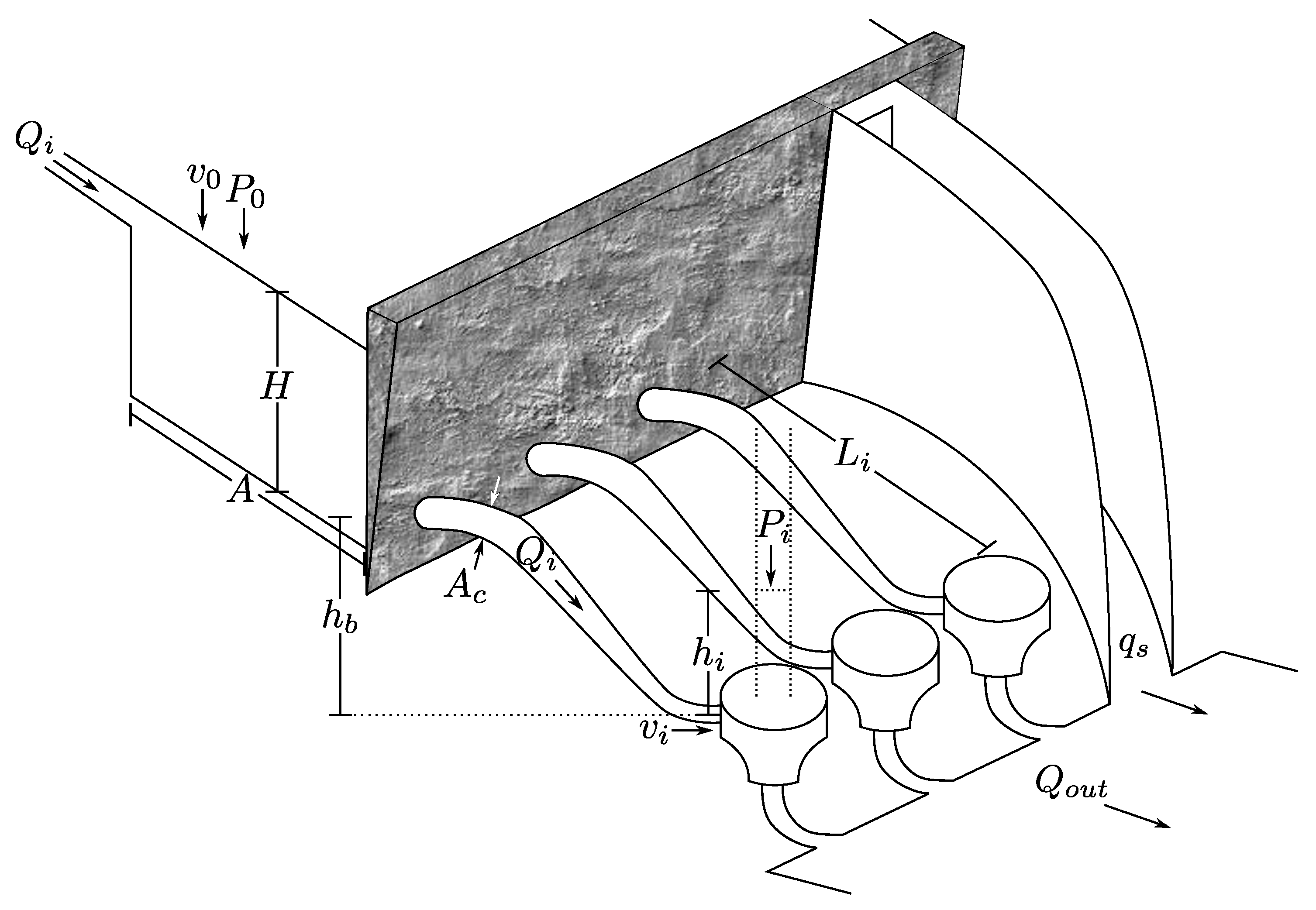
2. Dynamical Model
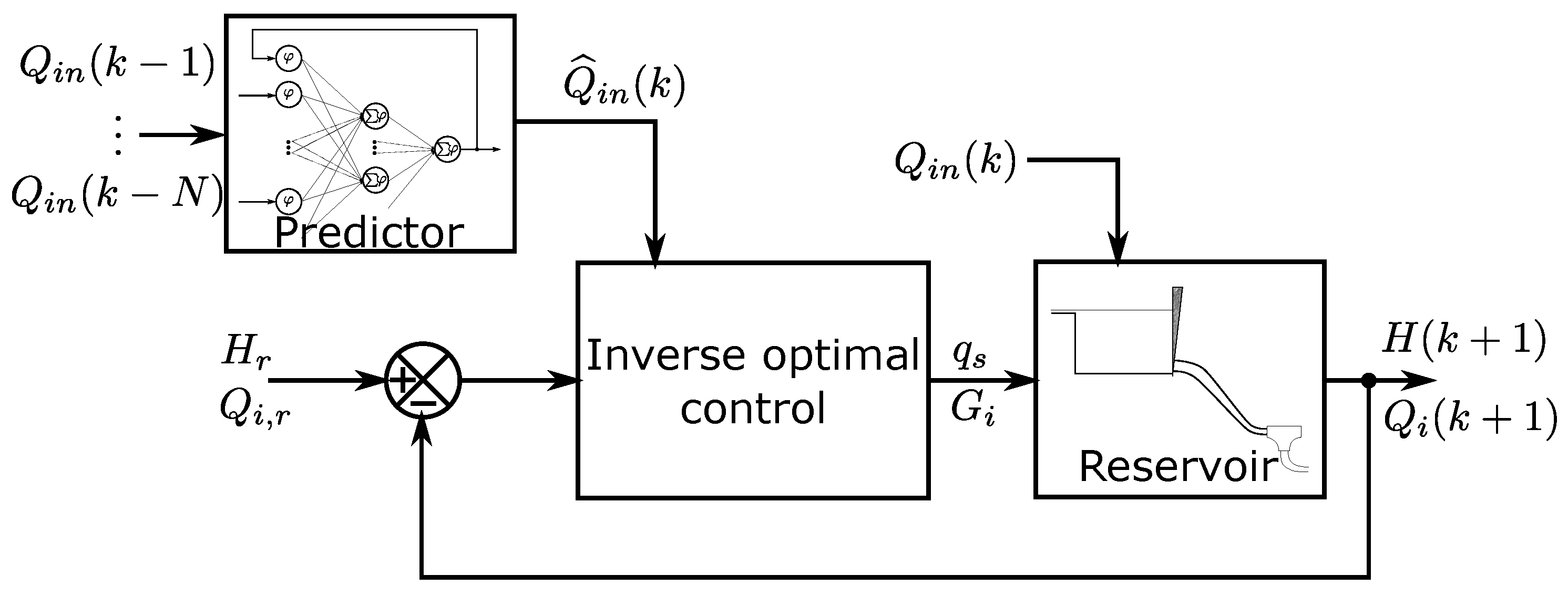
3. Inverse Optimal Control
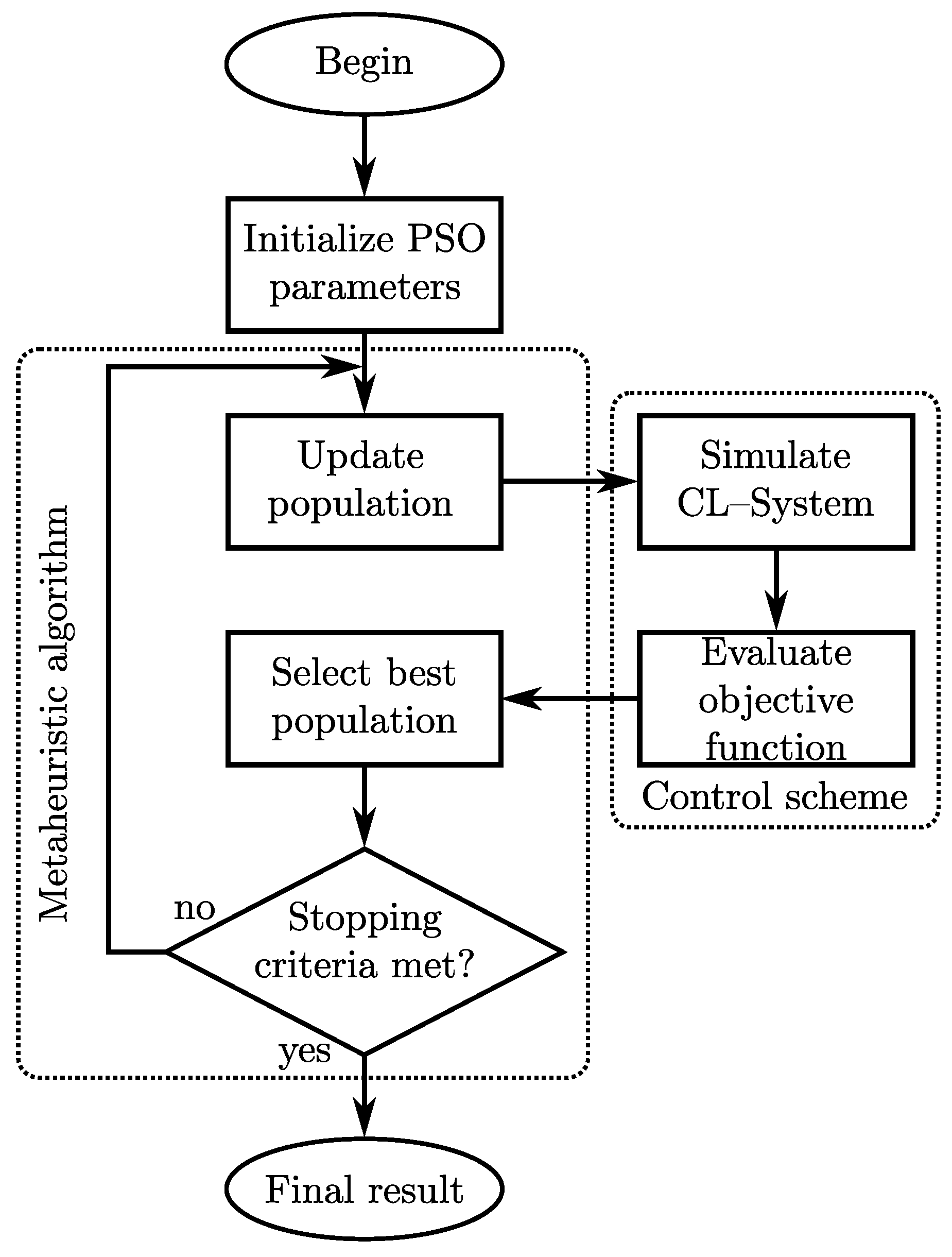
Metaheuristic Algorithm
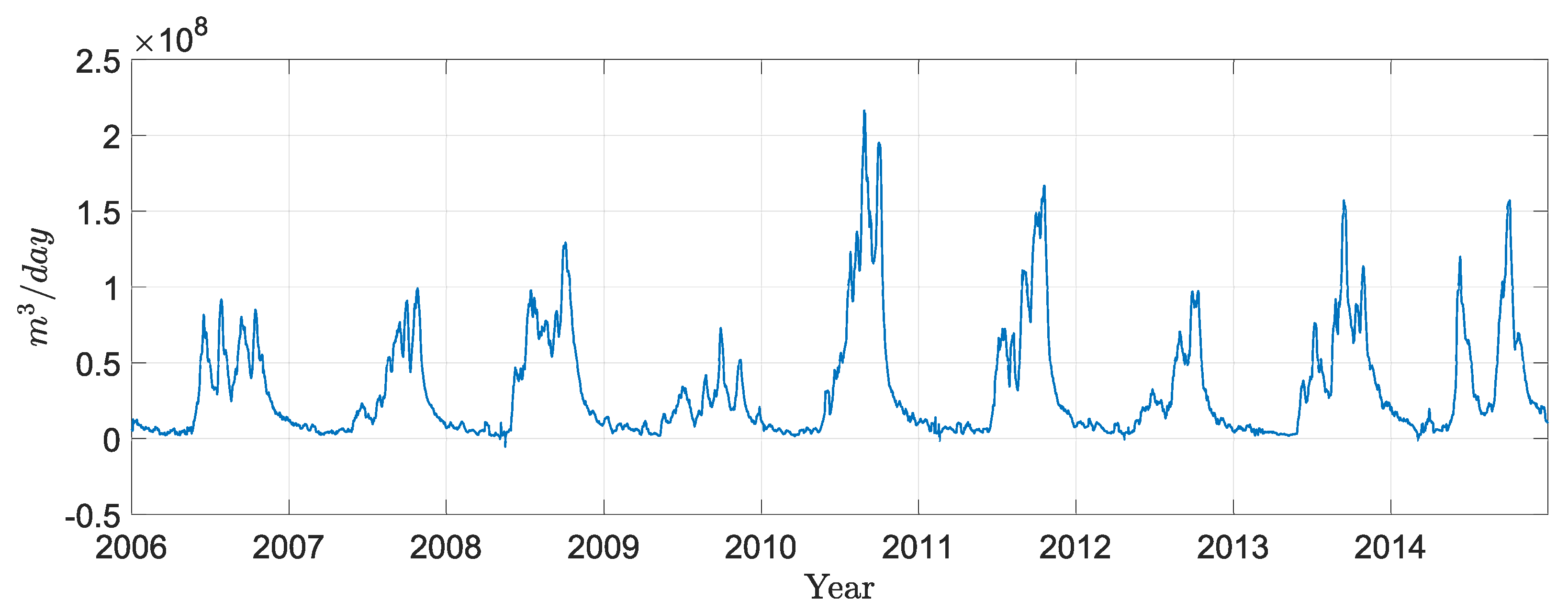
4. Forecasting
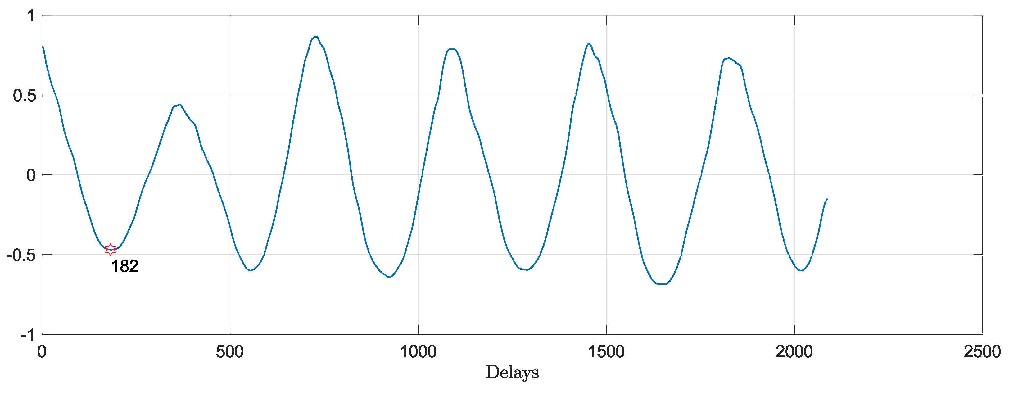
- The signal auto-correlation.Hypothesis 1.The auto-correlation indicates the number of sufficient inputs of previous data that have less relation with each other. In this way it does not fall into information redundancies.
- Order estimation of the system that generates the signal.Hypothesis 2.If the signal is a solution of a differential equation of order n, then, feedback outputs are sufficient.
- Signal frequency.Hypothesis 3.The number of hidden layers in the NN is directly proportional to the frequencies of the signal to be represented.
- Finally, the number of data to be predicted is considered, which is the number of outputs of the mentioned network.
5. Simulation
5.1. Tracking Control
5.2. Inverse Optimal Control including Parametric Variations
5.3. Inverse Optimal Control including External Disturbances
6. Results and Discussions
6.1. Model: Technical Considerations
6.2. Tracking Control
6.3. Inverse Optimal Control including Parametric Variations
6.4. Inverse Optimal Control including External Disturbances
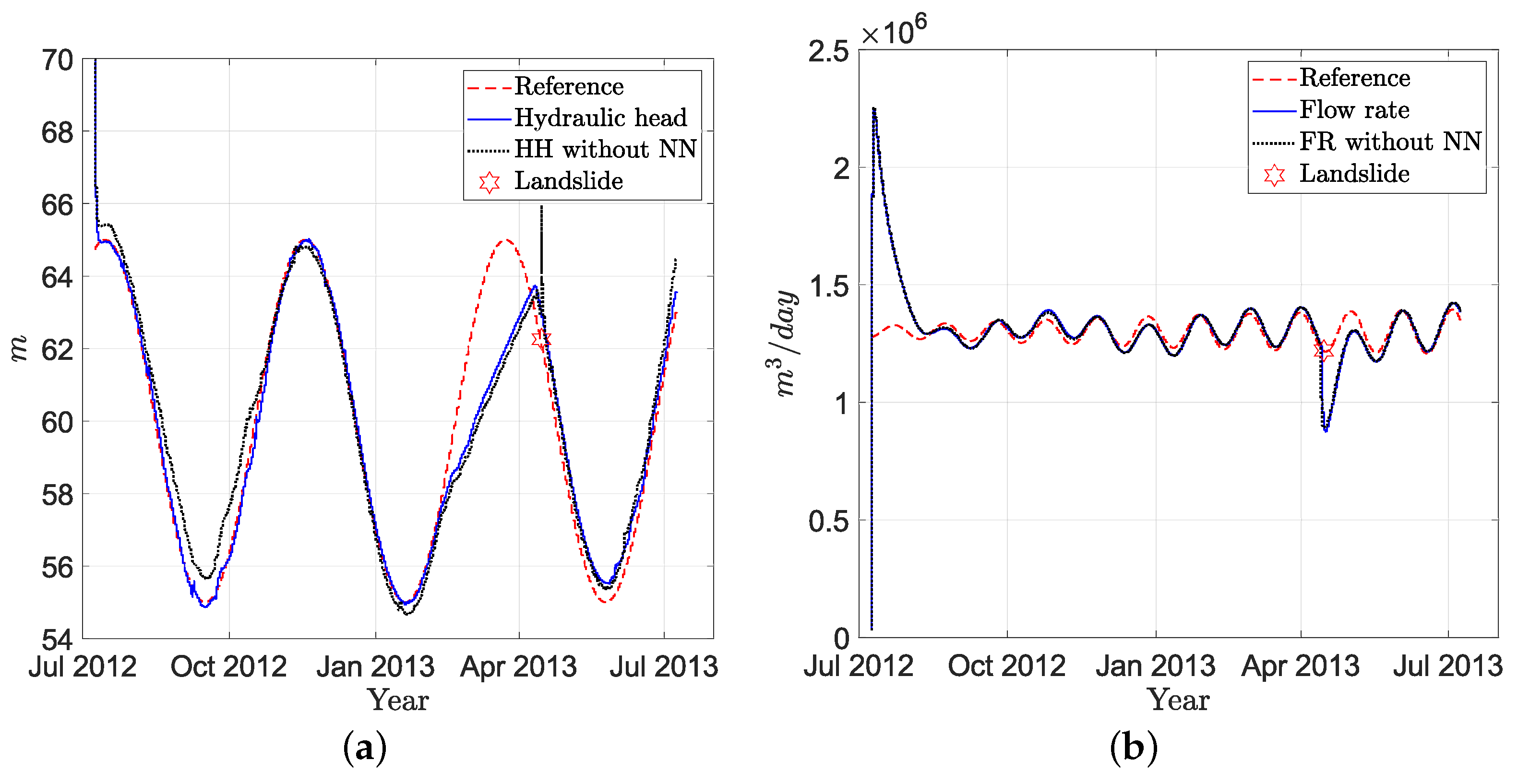
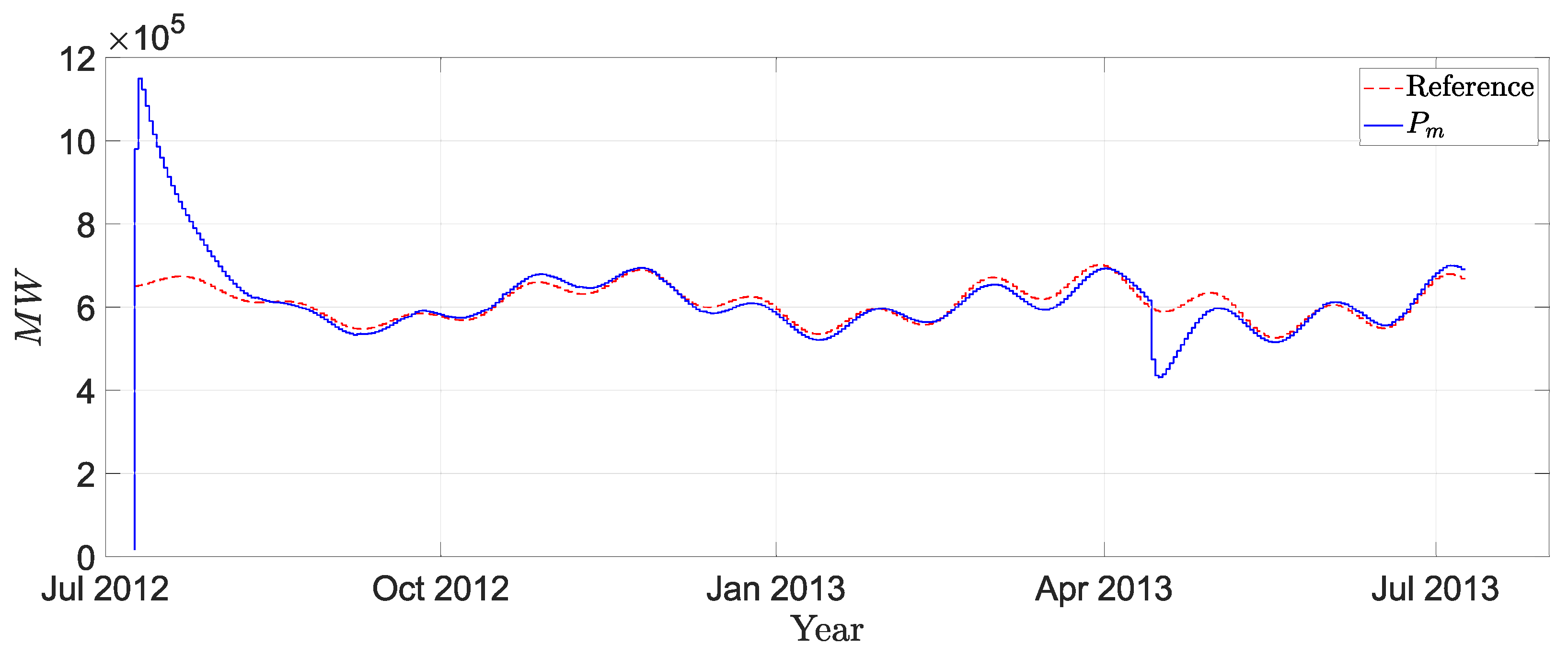
- The output in the hydraulic head should always be below the reference since it is considered that the controller input is always positive; this is, the flow is always unidirectional, Figure 10.
- Besides handling parametric variations (such as the case of landslides), the proposed Integral Action Inverse Optimal Controller scheme is also able to properly manage external perturbations; in fact, it is observed that the output of the controller does not differ significantly from the reference, Figure 10.
7. Conclusions
7.1. Tracking Control
7.2. Inverse Optimal Control including Parametric Variations
7.3. Inverse Optimal Control including External Disturbances
Author Contributions
Funding
Institutional Review Board Statement
Informed Consent Statement
Data Availability Statement
Acknowledgments
Conflicts of Interest
References
- Win, S.; Zin, W.W.; Kawasaki, A.; San, Z.M.L.T. Establishment of flood damage function models: A case study in the Bago River Basin, Myanmar. Int. J. Disaster Risk Reduct. 2018, 28, 688–700. [Google Scholar] [CrossRef]
- Sidle, R.C.; Greco, R.; Bogaard, T. Overview of landslide hydrology. Water 2019, 11, 148. [Google Scholar] [CrossRef] [Green Version]
- Morcillo, J.D.; Angulo, F.; Franco, C.J. Analyzing the hydroelectricity variability on power markets from a system dynamics and dynamic systems perspective: Seasonality and ENSO phenomenon. Energies 2020, 13, 2381. [Google Scholar] [CrossRef]
- Chanson, H. (Ed.) 2-Fundamentals of open channel flows. In Environmental Hydraulics of Open Channel Flows; Butterworth-Heinemann: Oxford, UK, 2004; pp. 11–34. [Google Scholar]
- Mahmoud, M.; Dutton, K.; Denman, M. Dynamical modelling and simulation of a cascaded reserevoirs hydropower plant. Electr. Power Syst. Res. 2004, 70, 129–139. [Google Scholar] [CrossRef]
- Robert, G.; Michaud, F. Hydro power plant modeling for generation control applications. In Proceedings of the 2012 American Control Conference (ACC), Montreal, QB, Canada, 27–29 June 2012; pp. 2289–2294. [Google Scholar]
- Moglen, G.E. Fundamentals of Open Channel Flow; CRC Press: Boca Raton, FL, USA, 2015. [Google Scholar]
- Blair, T.H. Energy Production Systems Engineering; John Wiley & Sons: Hoboken, NJ, USA, 2016. [Google Scholar]
- Huang, S.; Linyun, X.; Wang, J.; Li, P.; Wang, Z.; Ma, M. Fixed-time synergetic controller for stabilization of hydraulic turbine regulating system. Renew. Energy 2020, 157, 1233–1242. [Google Scholar] [CrossRef]
- Reigstad, T.I.; Uhlen, K. Variable speed hydropower conversion and control. IEEE Trans. Energy Convers. 2019, 35, 386–393. [Google Scholar] [CrossRef]
- Gil-González, W.J.; Garces, A.; Fosso, O.B.; Escobar-Mejía, A. Passivity-based control of power systems considering hydro-turbine with surge tank. IEEE Trans. Power Syst. 2019, 35, 2002–2011. [Google Scholar] [CrossRef]
- Sahin, E. Design of an Optimized Fractional High Order Differential Feedback Controller for Load Frequency Control of a Multi-Area Multi-Source Power System with Nonlinearity. IEEE Access 2020, 8, 12327–12342. [Google Scholar] [CrossRef]
- Singh, A.; Ghosh, S. Heuristic Optimization based Controller Design for Voltage Regulation in Small Hydropower Plant. In Proceedings of the 2020 First International Conference on Power, Control and Computing Technologies (ICPC2T), Raipur, India, 3–5 January 2020; pp. 111–116. [Google Scholar]
- Byrnes, C.; Lin, W. Losslessness, feedback equivalence, and the global stabilization of discrete-time nonlinear systems. IEEE Trans. Autom. Control 1994, 39, 83–98. [Google Scholar] [CrossRef]
- Gurubel, K.J.; Sanchez, E.N.; Coronado-Mendoza, A.; Zuniga-Grajeda, V.; Sulbaran-Rangel, B.; Breton-Deval, L. Inverse optimal neural control via passivity approach for nonlinear anaerobic bioprocesses with biofuels production. Optim. Control Appl. Methods 2019, 40, 848–858. [Google Scholar] [CrossRef]
- Gurubel, K.; Osuna-Enciso, V.; Coronado-Mendoza, A.; Cuevas, E. Optimal control strategy based on neural model of nonlinear systems and evolutionary algorithms for renewable energy production as applied to biofuel generation. J. Renew. Sustain. Energy 2017, 9, 033101. [Google Scholar] [CrossRef]
- Sanchez, E.N.; Ornelas-Tellez, F. Discrete-Time Inverse Optimal Control for Nonlinear Systems; CRC Press: Boca Raton, FL, USA, 2017. [Google Scholar]
- Morari, M. Robust stability of systems with integral control. IEEE Trans. Autom. Control 1985, 30, 574–577. [Google Scholar] [CrossRef] [Green Version]
- Ma, H.; Chen, M.; Wu, Q. Disturbance Observer-Based Inverse Optimal Tracking Control of the Unmanned Aerial Helicopter. In Proceedings of the 2019 IEEE 8th Data Driven Control and Learning Systems Conference (DDCLS), Dali, China, 24–27 May 2019; pp. 448–452. [Google Scholar]
- Min, X.; Li, Y.; Tong, S. Adaptive fuzzy output feedback inverse optimal control for vehicle active suspension systems. Neurocomputing 2020, 403, 257–267. [Google Scholar] [CrossRef]
- Djilali, L.; Sanchez, E.N.; Ornelas-Tellez, F.; Ruz-Hernandez, J.A.; Ricalde, L.J. Real-time neural inverse optimal control for low-voltage rid-through enhancement of double fed induction generator based wind turbines. ISA Trans. 2021, 113, 111–126. [Google Scholar] [CrossRef] [PubMed]
- Yang, S.; Yang, D.; Chen, J.; Zhao, B. Real-time reservoir operation using recurrent neural networks and inflow forecast from a distributed hydrological model. J. Hydrol. 2019, 579, 124229. [Google Scholar] [CrossRef]
- Ogliari, E.; Nespoli, A.; Mussetta, M.; Pretto, S.; Zimbardo, A.; Bonfanti, N.; Aufiero, M. A Hybrid Method for the Run-Of-The-River Hydroelectric Power Plant Energy Forecast: HYPE Hydrological Model and Neural Network. Forecasting 2020, 2, 410–428. [Google Scholar] [CrossRef]
- Benidis, K.; Rangapuram, S.S.; Flunkert, V.; Wang, B.; Maddix, D.; Turkmen, C.; Gasthaus, J.; Bohlke-Schneider, M.; Salinas, D.; Stella, L.; et al. Neural forecasting: Introduction and literature overview. arXiv 2020, arXiv:2004.10240. [Google Scholar]
- Zheng, A.; Casari, A. Feature Engineering for Machine Learning: Principles and Techniques for Data Scientists; O’Reilly Media, Inc.: Sebastopol, CA, USA, 2018. [Google Scholar]
- Tutz, G.; Ramzan, S. Improved methods for the imputation of missing data by nearest neighbor methods. Comput. Stat. Data Anal. 2015, 90, 84–99. [Google Scholar] [CrossRef] [Green Version]
- Smith, S.W. (Ed.) Chapter 15—Moving Average Filters. In Digital Signal Processing; Newnes: Boston, MA, USA, 2003; pp. 277–284. [Google Scholar] [CrossRef]
- Babu, C.N.; Reddy, B.E. A moving-average filter based hybrid ARIMA–ANN model for forecasting time series data. Appl. Soft Comput. 2014, 23, 27–38. [Google Scholar] [CrossRef]
- Wilcox, R. (Ed.) Chapter 3—Estimating Measures of Location and Scale. In Introduction to Robust Estimation and Hypothesis Testing, 4th ed.; Statistical Modeling and Decision Science; Academic Press: Cambridge, MA, USA, 2017; pp. 45–106. [Google Scholar] [CrossRef]
- Kuhn, M.; Johnson, K. Feature Engineering and Selection: A Practical Approach for Predictive Models; CRC Press: Boca Raton, FL, USA, 2019. [Google Scholar]
- Yeo, I.K.; Johnson, R.A. A new family of power transformations to improve normality or symmetry. Biometrika 2000, 87, 954–959. [Google Scholar] [CrossRef]
- Kennedy, J.; Eberhart, R. Particle swarm optimization. In Proceedings of the ICNN’95—International Conference on Neural Networks, Perth, WA, Australia, 27 November–1 December 1995; Volume 4, pp. 1942–1948. [Google Scholar]
- Eberhart, R.; Kennedy, J. A new optimizer using particle swarm theory. In Proceedings of the Sixth International Symposium on Micro Machine and Human Science, Nagoya, Japan, 4–6 October 1995; pp. 39–43. [Google Scholar]
- Yarpiz. Particle Swarm Optimization (PSO) in MATLAB—Video Tutorial. 2016. Available online: https://yarpiz.com/440/ytea101-particle-swarm-optimization-pso-in-matlab-video-tutorial (accessed on 28 June 2021).


| Constant | Value |
|---|---|
| 0.01 | |
| 0.99 | |
| 0.01 | |
| 0.99 | |
| 2 days | |
| 3285 days | |
| 20 days | |
| 3267 days |
| Parameter | Description | Value |
|---|---|---|
| N | population | 500 particles |
| personal acceleration coefficient | 2 | |
| social acceleration coefficient | 2 | |
| w | inertia coefficient | 1 |
| damping ratio of inertia coefficient | 0.99 |
| Attribute | Value |
|---|---|
| count | 3202 |
| mean | 30.882717 |
| std | 39.399464 |
| min | −73.790000 |
| max | 299.740000 |
| missed | 85 |
| Attribute | Value |
|---|---|
| count | 3287 |
| mean | 31.8105 |
| std | 35.8087 |
| min | −0.7090 |
| max | 216.3110 |
Publisher’s Note: MDPI stays neutral with regard to jurisdictional claims in published maps and institutional affiliations. |
© 2021 by the authors. Licensee MDPI, Basel, Switzerland. This article is an open access article distributed under the terms and conditions of the Creative Commons Attribution (CC BY) license (https://creativecommons.org/licenses/by/4.0/).
Share and Cite
Perez-Villalpando, M.A.; Gurubel Tun, K.J.; Arellano-Muro, C.A.; Fausto, F. Inverse Optimal Control Using Metaheuristics of Hydropower Plant Model via Forecasting Based on the Feature Engineering. Energies 2021, 14, 7356. https://doi.org/10.3390/en14217356
Perez-Villalpando MA, Gurubel Tun KJ, Arellano-Muro CA, Fausto F. Inverse Optimal Control Using Metaheuristics of Hydropower Plant Model via Forecasting Based on the Feature Engineering. Energies. 2021; 14(21):7356. https://doi.org/10.3390/en14217356
Chicago/Turabian StylePerez-Villalpando, Marlene A., Kelly J. Gurubel Tun, Carlos A. Arellano-Muro, and Fernando Fausto. 2021. "Inverse Optimal Control Using Metaheuristics of Hydropower Plant Model via Forecasting Based on the Feature Engineering" Energies 14, no. 21: 7356. https://doi.org/10.3390/en14217356
APA StylePerez-Villalpando, M. A., Gurubel Tun, K. J., Arellano-Muro, C. A., & Fausto, F. (2021). Inverse Optimal Control Using Metaheuristics of Hydropower Plant Model via Forecasting Based on the Feature Engineering. Energies, 14(21), 7356. https://doi.org/10.3390/en14217356