Full-Order Terminal Sliding-Mode Control of Brushless Doubly Fed Induction Generator for Ship Microgrids

Abstract

This paper proposes a full-order terminal sliding-mode (FOTSM) control scheme for brushless doubly fed induction generator (BDFIG)-based islanded microgrids. To deal with mismatched uncertainties in the BDFIG system, virtual control technique-based full-order sliding-mode control is applied to stabilize the amplitude and frequency of terminal voltage. In the current loops, two full-order terminal sliding-mode controllers are designed to make sure that the current tracking errors can reach their equilibrium points in finite time. It is demonstrated by the comprehensive simulations that the proposed method can significantly improve the tracking accuracy, the rapidness, and the robustness to the uncertainties of the BDFIG control system and can enhance the output voltage quality. Furthermore, an experimental study of the proposed control method for BDFIG-based islanded microgrids would be another important future work.

1. Introduction

The brushless doubly fed induction generator (BDFIG) has demonstrated promising prospects in the energy-saving performance of microgrids, such as applications in wind power systems, ship shaft power generation systems, etc. Among the members of the induction motor (IM) family, the BDFIG has no brushes and slip rings, which is the main difference from the traditional doubly fed induction generator (DFIG) [1,2,3]. The BDFIG not only inherits the merits of the DFIG but also shows higher reliability and longer work lifetime. Therefore, it has been regarded as a feasible alternative [4,5].

The BDFIG consists of a rotor and two stator windings with different pole pairs. The indirect electromagnetic coupling effect between the two stator is generated via a specially designed squirrel-cage type rotor without the rotor voltage [6,7]. The BDFIG-based system for a ship microgrid is depicted in Figure 1. The BDFIG is connected to the main engine of the ship, the power winding (PW) is directly joined to the grid, while the control winding (CW) is supplied by a back-to-back converter achieving the bidirectional power flow [8]. The PW-side converter maintains the stability of the DC-bus voltage, and the CW-side converter regulates the frequency variable exciting current.

The control strategies proposed for BDFIGs include the typical vector control (VC) [9]; the direct torque control (DTC) [10]; and some others such as the phase angle control [11], indirect stator quantity control [12], etc. The DTC has advantages such as rapidness and robustness under operating conditions, but large torque/power ripples and current-waveform distortions will degrade the quality of the output power [13]. While in the VC system, the current harmonic spectra are better than those under the DTC. However, the common controllers are sensitive to inner parameter perturbation and external disturbances. The controller design for the BDFIG-based microgrid is somewhat difficult to develop for the following two main reasons: $\left(1\right)$ the mathematical model of the BDFIG is a class of highly nonlinear multi-input-multi-output (MIMO) systems with unavoidable uncertainties and lots of degrees of freedom; $\left(2\right)$ the parameters of the PW, the CW, and the rotor vary with current frequency, motor temperature, and magnetic saturation effect. The existing controller design algorithms are generally heavy parameter-dependence, meanwhile common and practical proportional-integral (PI) control cannot meet the requirements of control objectives well in the precision and dynamic performance [14,15]. Therefore, it is necessary to design advanced nonlinear controllers to compensate for the influence of parameter variations in the system, so that the BDFIG-based microgrid can obtain a good operating performance in various environments and conditions.

With the development of control theory, lots of control methods for DFIG systems have been proposed to implement high-performance control for the BDFIG, such as backstepping control [16], adaptive control [17], $H\infty$ control [18], fuzzy control [19], model reference adaptive control (MRAC) [20], model predictive control (MPC) [21], active disturbance rejection control (ADRC) [22,23,24], neural network control [25], sliding-mode control (SMC) [26], etc.

Due to the low sensitivity to parameter perturbations and the strong robustness to external disturbance, the sliding mode control (SMC) is proposed for the IM [27,28], the DFIG [29], and the BDFIGs [30]. An integral sliding-mode-based DTC scheme is proposed for DFIG-based wind-energy conversion systems in [31], and the advantages against parameter variations is illustrated. However, the convergence is not finite and undesired chattering exists. To deal with the chattering problem, an adaptive internal SMC is developed to optimize the efficiency of variable-speed wind turbines and to meet the control requirements of wind energy conversion systems under model uncertainties, which generates smoothed active power with minimized ripple [32]. However, a discrete control output with a high switching frequency is needed when applying this method. Alternatively, the second-order SMC can eliminate chattering without a discrete output [33,34]. However, the mathematical calculations of this method are complex and the implementation becomes difficult in the case of the increasing states [35]. A saturation function-based integral SMC with feed-forward terms is proposed for the BDFIG, but a quasi-sliding mode controller utilizing the boundary layer would decrease the control accuracy [36]. In [34], a super twisting sliding mode direct power control scheme for the BDFIGs is implemented. Although the super twisting SMC is an effective way to suppress the chattering with continuous signals, it is non-monotonically convergent to the sliding manifold and may cause a large overshoot [37].

The mathematical model of the BDFIG is a class of second-order nonlinear systems with matched and mismatched uncertainties. However, the SMC in general is regarded as an excellent method for nonlinear systems, while until now, most SMC methods depended on the so-called matched conditions [31]. The reference of $d$- and $q$- currents designed by the traditional SMC contains high-frequency switching signals, and its derivative existing in the signals of space vector pulse width modulation (SVPWM) would lead to the singularity problem. In existing works, little attention has been paid to this issue. Therefore, to improve the accuracy rapidness and robustness to the uncertainties, advanced control methods for the BDFIGs are demanded to have a strong disturbance rejection capability for mismatched uncertainties.

The full-order terminal sliding-mode (FOTSM) is one of the most recent proposed SMC theory, which is proven to be efficient for mismatched nonlinear systems [38]. By introducing the ideal of both the full-order terminal sliding-mode (FOTSM) control algorithm and the virtual control technique, this paper proposes a novel FOTSM-based control method to stabilize the amplitude and frequency of terminal voltage under the parameter perturbation and electrical load vary. The main contributions in this article can be summarized as follows:

(1) Compared with the conventional controllers, the control precision and transient response of the amplitude and frequency of terminal voltage improved by adopting the proposed FOTSM controllers without using low pass filters or the boundary layer method.

(2) On the premise that the excellent anti-disturbance of the SMC is kept in case of uncertainties, the chattering in the conventional SMC is mitigated by the integral control law and continuous pulse width modulation (PWM) output signals can be generated.

(3) The matched and mismatched uncertainties in the BDFIG system are adequately considered and thoroughly compensated. The adaptive gain is utilized to avoid overestimating the upper bound of the uncertainties and to improve the adaptation of the BDFIG system to the uncertainties.

This paper is organized as follows: Section 2 introduces the mathematical model of the BDFIG with uncertainties. In Section 3, the voltage amplitude- and current-loop controllers based on FOTSM are designed. Section 4 gives the simulation results. Finally, the conclusions are summarized in Section 5.

2. Preliminary

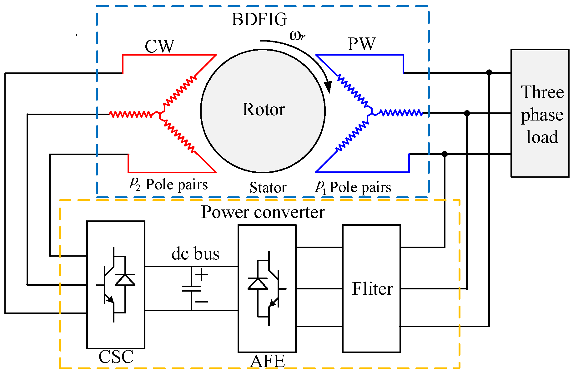
2.1. Dynamic Model of the BDFIG

The dynamic mathematical model of the BDFIG in the d-q coordinate with the angle frequency ${\omega }_2$ of the rotating can be expressed as

$$\left\{\begin{array}{c}\hfill u_{1d}=R_1{i}_{1d}+s{\varphi }_{1d}-{\omega }_2{\varphi }_{1q}\\ \hfill u_{1q}=R_1{i}_{1q}+s{\varphi }_{1q}+{\omega }_2{\varphi }_{1d}\end{array}\right.$$

(1)

$$\left\{\begin{array}{c}\hfill u_{2d}=R_2{i}_{2d}+s{\varphi }_{2d}-[{\omega }_2-(p_1+p_2){\omega }_r]{\varphi }_{2q}\\ \hfill u_{2q}=R_2{i}_{2q}+s{\varphi }_{2q}+[{\omega }_2-(p_1+p_2){\omega }_r]{\varphi }_{2d}\end{array}\right.$$

(2)

$$\left\{\begin{array}{c}\hfill u_{rd}=R_r{i}_{rd}+s{\varphi }_{rd}-({\omega }_2-p_1{\omega }_r){\varphi }_{rq}\\ \hfill u_{rq}=R_r{i}_{rq}+s{\varphi }_{rq}+({\omega }_2-p_1{\omega }_r){\varphi }_{rd}\end{array}\right.$$

(3)

$$\left\{\begin{array}{c}\hfill {\varphi }_{1d}=L_1{i}_{1d}+L_{1r}{i}_{rd}\\ \hfill {\varphi }_{1q}=L_1{i}_{1q}+L_{1r}{i}_{rq}\end{array}\right.$$

(4)

$$\left\{\begin{array}{c}\hfill {\varphi }_{2d}=L_2{i}_{2d}+L_{2r}{i}_{rd}\\ \hfill {\varphi }_{2q}=L_2{i}_{2q}+L_{2r}{i}_{rq}\end{array}\right.$$

(5)

$$\left\{\begin{array}{c}\hfill {\varphi }_{rd}=L_r{i}_{rd}+L_{1r}{i}_{1d}+L_{2r}{i}_{2d}\\ \hfill {\varphi }_{rq}=L_r{i}_{rq}+L_{1r}{i}_{1q}+L_{2r}{i}_{2q}\end{array}\right.$$

(6)

and the rotor speed of the BDFIG can be expressed as

$${\omega }_1+{\omega }_2\widetilde{=}(p_1+p_2){\omega }_r.$$

(7)

Setting the rotor voltages to zero $u_{rd}=u_{rq}=0$, the voltage equation of rotor (3) can be rewritten as

$$\left\{\begin{array}{c}\hfill 0=R_r{i}_{rd}+s{\varphi }_{rd}-[{\omega }_2-p_1{\omega }_r]{\varphi }_{rq}\\ \hfill 0=R_r{i}_{rq}+s{\varphi }_{rq}+[{\omega }_2-p_1{\omega }_r]{\varphi }_{rd}\end{array}\right..$$

(8)

Substituting (6) and (7) into (8) yields

$$\begin{array}{cc}\hfill i_{rd}=& -\frac{[L_r{s}^2+R_{r}s+L_r{({\omega }_1-p_2{\omega }_2)}^2](L_{1r}{i}_{1d}+L_{2r}{i}_{2d})}{{(R_r+L_{r}s)}^2+L_r^2{({\omega }_1-p_2{\omega }_r)}^2}\hfill \\ \hfill & -\frac{R_r({\omega }_1-p_2{\omega }_r)(L_{1r}{i}_{1q}+L_{2r}{i}_{2q})}{{(R_r+L_{r}s)}^2+L_r^2{({\omega }_1-P_2{\omega }_r)}^2}\hfill \end{array}$$

(9)

$$\begin{array}{cc}\hfill i_{rq}=& \frac{{\omega }_1-p_2{\omega }_r}{R_r+L_{r}s}[1-\frac{L_r^2{s}^2+L_r{R}_{r}s+L_r^2{({\omega }_1-p_2{\omega }_r)}^2}{{(R_r+L_{r}s)}^2+L_r^2{({\omega }_1-p_2{\omega }_r)}^2}](L_{1r}{i}_{1d}+L_{2r}{i}_{2d})\hfill \\ \hfill & -\frac{1}{R_r+L_{r}s}(L_{1r}{i}_{1q}+L_{2r}{i}_{2q})[s+\frac{L_r{R}_r{({\omega }_1-p_2{\omega }_r)}^2}{{(R_r+L_{r}s)}^2+L_r^2{({\omega }_1-p_2{\omega }_r)}^2}].\hfill \end{array}$$

(10)

In general, the values of $R_r$ are close to $L_r$. According to (7), the rotor speed range is limited. Hence, the ${\omega }_2$ is generally limited to $30\%$ of ${\omega }_1$. Therefore, the first term of (9) can be rewritten as

$$i_{rd}=-\frac{[s^2+(R_r/L_r)s+{({\omega }_1-p_2{\omega }_2)}^2](L_{1r}{i}_{1d}+L_{2r}{i}_{2d})}{L_r[s^2+2(R_r/L_r)s+{({\omega }_1-p_2{\omega }_r)}^2]}.$$

(11)

Considering that the zeroes and poles of this term can cancel each other, the Equation (11) can be simplified as

$$i_{rd}=-\frac{L_{1r}{i}_{1d}+L_{2r}{i}_{rd}}{L_r}-\frac{R_r(L_{1r}{i}_{1q}+L_{2r}{i}_{2q})}{L_r^2({\omega }_1-p_2{\omega }_r)}.$$

(12)

Similarly, Equation (10) can be simplified as

$$i_{rq}=-\frac{L_{1r}{i}_{1q}+L_{2r}{i}_{2q}}{L_r}.$$

(13)

According to (12) and (13), the voltage function of the CW (2) can be rewritten as

$$\frac{\mathrm{d}{i}_{2d}}{\mathrm{d}t}={\sigma }_2{L}_2(u_{2d}-R_2{i}_{2d}+D_{2d})$$

(14)

$$\frac{\mathrm{d}{i}_{2q}}{\mathrm{d}t}={\sigma }_2{L}_2(u_{2q}-R_2{i}_{2q}+D_{2q})$$

(15)

where $D_{2d}={\alpha }_1{i}_{2q}+{\alpha }_2{i}_{1d}+{\alpha }_3{i}_{1q}$, $D_{2q}={\alpha }_4{i}_{2d}+{\alpha }_5{i}_{1d}+{\alpha }_6{i}_{1q}$, ${\sigma }_2=1-L_{2r}^2/\left(L_2{L}_r\right)$,

$$\begin{array}{cc}\hfill {\alpha }_1& =-\frac{{\omega }_1({\omega }_1-p_2{\omega }_r)(L_r^2{L}_2+L_{2r}^2{L}_r)-L_{2r}^2{R}_{r}s}{L_r^2({\omega }_1-p_2{\omega }_r)},{\alpha }_2=\frac{L_{1r}{L}_{2r}s}{L_r},\hfill \\ \hfill {\alpha }_3& =-\frac{L_{1r}{L}_{2r}[R_{r}s+L_r{\omega }_1({\omega }_1-p_2{\omega }_r)]}{L_r^2({\omega }_1-p_2{\omega }_r)},{\alpha }_4=\frac{{\sigma }_2{L}_2{L}_r{\omega }_1}{L_1},\hfill \\ \hfill {\alpha }_5& =-\frac{{\omega }_1{L}_{1r}{L}_{2r}}{L_r},{\alpha }_6=-\frac{L_{1r}{L}_{2r}[{\omega }_1{R}_r-L_r({\omega }_1-p_2{\omega }_{r}s)]}{L_r^2({\omega }_1-p_2{\omega }_r)}.\hfill \end{array}$$

The currents of CW are assumed as $i_{2q}=0$, $i_{2d}=I_2$. Substituing (14) and (15) into (1), the voltage of the PW can be expressed as

$$u_{1d}=R_1{i}_{1d}+\frac{{\omega }_2(L_{1r}^2-L_1{L}_r)}{L_r}{i}_{1q}$$

(16)

$$u_{1q}=R_1{i}_{1q}-\frac{{\omega }_2(L_{1r}^2-L_1{L}_r)}{L_r}{i}_{1d}-\frac{{\omega }_2{L}_{1r}{L}_{2r}}{L_r}{I}_2.$$

(17)

The PW voltage can be calculated by

$$\begin{array}{cc}\hfill U_1& =\sqrt{u_{1d}^2+u_{1q}^2}\hfill \\ \hfill & =\{{({\omega }_2\frac{L_{1r}{L}_{2r}}{L_r})}^2{I}_2^2-\frac{2{\omega }_2{L}_{1r}{L}_{2r}}{L_r}[({\omega }_2{L}_1-\frac{{\omega }_2{L}_{1r}^2}{L_r})i_{1d}+R_1{i}_{1q}]I_2\hfill \\ \hfill & +R_1^2(i_{1d}^2+i_{1q}^2)+({\omega }_2{L}_1-\frac{{\omega }_2{L}_{1r}^2}{L_r})(i_{1d}^2+i_{1q}^2){\}}^{1/2}.\hfill \end{array}$$

(18)

For a small perturbation in the control output $\mathrm{\Delta }{I}_2$, Equation (18) can be described by

$$U_1(I_{2E}+\mathrm{\Delta }{I}_2)=U_1\left(I_{2E}\right)+\mathrm{\Delta }{I}_2\frac{\mathrm{d}\mathrm{\Delta }{U}_1}{\mathrm{d}t}{|}_{I_2=I_{2E}}$$

(19)

where $I_{2E}$ is the amplitude of a steady-state value of the CW current. Then, considering (18) and (19) yields

$$\begin{array}{cc}\hfill \mathrm{\Delta }{U}_1& =U_1(I_{2E}+{\mathrm{\Delta }}_{I_2})-U\left(I_{2E}\right)\hfill \\ \hfill & =U_1(I_{2E}+\mathrm{\Delta }{I}_2)-U_{1ref}\hfill \\ \hfill & =K_u\mathrm{\Delta }{I}_{2E}\hfill \end{array}$$

(20)

where $K_u={\omega }_2{L}_{1r}{L}_{2r}[{\omega }_2{L}_{1r}{L}_{2r}{I}_{2E}+{\omega }_2(L_{1r}^2-L_1{L}_r)i_{1d}-R_1{L}_{1r}{i}_{1q}]$ is a constant in the steady-state. According to (19), the amplitude of the steady-state value of CW current can be calculated as

$$I_{2E}=[({\beta }_1{i}_{1d}+R_1{i}_{1q})+{(2{\beta }_1{R}_1{i}_{1d}{i}_{1q}-R_1^2{i}_{1d}^2-{\beta }_1^2{i}_{1q}^2+U_{ref})}^{1/2}]/{\beta }_2$$

(21)

where ${\beta }_1={\omega }_2(L_1-L_{1r}^2/L_r)$, ${\beta }_2={\omega }_2{L}_{1r}{L}_{2r}/L_r$.

2.2. Outer Loop Subsystem

The outer-loop subsystem is the PW-voltage loop. The tracking error can be defined as $e_U=U_{1ref}-U_1$. According to the mathematical model of the BDFIG, the voltage tracking error dynamics can be expressed by

$$\begin{array}{c}\hfill {\dot{e}}_U={\dot{U}}_{ref}-{\dot{U}}_1=-K_u\mathrm{\Delta }{\dot{I}}_2.\end{array}$$

(22)

Considering the change in temperature and frequency, the variation of resistance and inductance can be represented by

$$\left\{\begin{array}{c}{R}_i=R_{i0}+\mathrm{\Delta }{R}_{i}i=1,2,r\hfill \\ L_j=L_{j0}+\mathrm{\Delta }{L}_{j}j=1,2,r,1r,2r\hfill \end{array}\right.$$

(23)

Furthermore,

$$\left\{\begin{array}{cc}\hfill {\sigma }_2& ={\sigma }_{20}+\mathrm{\Delta }{\sigma }_2\hfill \\ \hfill {\beta }_k& ={\beta }_{k0}+\mathrm{\Delta }{\beta }_{k}k=1,2\hfill \\ \hfill {\alpha }_m& ={\alpha }_{m0}+\mathrm{\Delta }{\alpha }_{m}m=1,\dots ,9\hfill \\ \hfill T_1& =R_2{\sigma }_2{L}_2=T_{10}+\mathrm{\Delta }{T}_1\hfill \\ \hfill T_2& ={\sigma }_2{L}_2=T_{20}+\mathrm{\Delta }{T}_2\hfill \end{array}\right..$$

(24)

The above uncertainties can be assumed to be bounded; therefore,

$$\left\{\begin{array}{c}\left|\mathrm{\Delta }{R}_i\right|\le M_{R_i}i=1,2,r\hfill \\ \left|\mathrm{\Delta }{L}_j\right|\le M_{L_j}j=1,2,r,1r,2r\hfill \end{array}\right.$$

(25)

Furthermore,

$$\left\{\begin{array}{cc}\hfill \left|\mathrm{\Delta }{\sigma }_2\right|& \le M_{{\sigma }_2}\hfill \\ \hfill \left|\mathrm{\Delta }{\beta }_k\right|& \le M_{{\beta }_k}k=1,2\hfill \\ \hfill \left|\mathrm{\Delta }{\alpha }_m\right|& \le M_{{\alpha }_m}m=1,\dots ,9\hfill \\ \hfill \left|\mathrm{\Delta }{T}_n\right|& \le M_{T_n}n=1,2\hfill \end{array}\right.$$

(26)

where $M_{R_j}$, $M_{L_k}$, $M_{{\sigma }_2}$, $M_{{\beta }_1}$, and $M_{{\beta }_2}$ are known to be positive constants.

Therefore, considering the parameter perturbation, the error dynamics in the outer-loop can be described by

$$\begin{array}{cc}\hfill {\dot{e}}_U& =-K_u\mathrm{\Delta }{\dot{I}}_2\hfill \\ \hfill & =-{\omega }_2(L_{1r0}+\mathrm{\Delta }{L}_{1r})(L_{2r0}+\mathrm{\Delta }{L}_{2r})\left[\begin{array}{c}{\omega }_2(L_{1r0}+\mathrm{\Delta }{L}_{1r})(L_{2r0}+\mathrm{\Delta }{L}_{2r})I_{2E}\hfill \\ +{\omega }_2{(L_{1r0}+\mathrm{\Delta }{L}_{1r})}^2{i}_{1d}\hfill \\ -{\omega }_2(L_{1r0}+\mathrm{\Delta }{L}_{1r})(L_{r0}+\mathrm{\Delta }{L}_r)i_{1d}\hfill \\ -(R_{10}+\mathrm{\Delta }{R}_1)(L_{10}+\mathrm{\Delta }{L}_1)i_{1q}\hfill \end{array}\right]\mathrm{\Delta }{\dot{I}}_2.\hfill \end{array}$$

(27)

The virtual control law is defined by

$$i_{2dref}=\mathrm{\Delta }{I}_{2ref}+I_{2E}.$$

(28)

The current tracking error of $i_d$ is defined as

$$e_{id}=i_{dref}-i_d.$$

(29)

Thus, the tracking error dynamics (22) can be expressed as

$${\dot{e}}_U=-K_{u0}\mathrm{\Delta }{\dot{I}}_{2ref}-\mathrm{\Delta }{K}_u\mathrm{\Delta }{\dot{I}}_{2ref}+K_{u0}{\dot{e}}_{id}$$

(30)

where $K_{u0}={\omega }_2{L}_{1r0}{L}_{2r0}[{\omega }_2{L}_{1r0}{L}_{2r0}{I}_{2E}+{\omega }_2(L_{1r0}^2-L_{10}{L}_{r0})i_{1d}-R_{10}{L}_{1r0}{i}_{1q}]$ and $\mathrm{\Delta }{K}_u\mathrm{\Delta }{\dot{I}}_{2ref}$ is defined as the coefficient of uncertain control gain in the control system of the BDFIG.

For analyzing the lumped unmatched uncertainty ${\rho }_0$, the following uncertainties are defined as

$${\delta }_U=\frac{\mathrm{\Delta }{K}_u}{K_{u0}}=\frac{K_u-K_{u0}}{K_{u0}}$$

(31)

which is upper-bounded by

$$\left|{\delta }_U\right|\le M_{\delta }<1.$$

(32)

2.3. Inner Loop Subsystem

According to (14) and (15), the inner-loop current subsystem can be obtained by

$$\frac{\mathrm{d}{\mathit{i}}_{2dq}}{\mathrm{d}t}={\mathit{F}}_0{\mathit{i}}_{2dq}+\mathit{G}({\mathit{u}}_{2dq}+{\mathit{F}}_1{\mathit{i}}_{2dq}+{\mathit{F}}_2{\mathit{i}}_{1dq})$$

(33)

where ${\mathit{i}}_{2dq}={[i_{2d},i_{2q}]}^T$, ${\mathit{u}}_{2dq}={[u_{2d},u_{2q}]}^T$, ${\mathit{F}}_0={\mathit{F}}_{00}+\mathrm{\Delta }{\mathit{F}}_0$, $\mathit{G}={\mathit{G}}_0+\mathrm{\Delta }\mathit{G}$, ${\mathit{F}}_1={\mathit{F}}_{10}+\mathrm{\Delta }{\mathit{F}}_1$, ${\mathit{F}}_{20}={\mathit{F}}_{20}+\mathrm{\Delta }{\mathit{F}}_2$,

$$\begin{array}{c}{\mathit{F}}_{00}=-\left[\begin{array}{cc}{T}_{10}& 0\\ 0& T_{10}\end{array}\right],{\mathit{G}}_0=\left[\begin{array}{cc}{T}_{20}& 0\\ 0& T_{20}\end{array}\right],{\mathit{F}}_{10}=\left[\begin{array}{cc}0& {\alpha }_{10}\\ {\alpha }_{40}& 0\end{array}\right],{\mathit{F}}_{20}=\left[\begin{array}{cc}{\alpha }_{20}& {\alpha }_{50}\\ {\alpha }_{30}& {\alpha }_{60}\end{array}\right],\hfill \\ \mathrm{\Delta }{\mathit{F}}_0=-\left[\begin{array}{cc}\mathrm{\Delta }{T}_1& 0\\ 0& \mathrm{\Delta }{T}_1\end{array}\right],\mathrm{\Delta }\mathit{G}=\left[\begin{array}{cc}\mathrm{\Delta }{T}_2& 0\\ 0& \mathrm{\Delta }{T}_2\end{array}\right],\mathrm{\Delta }{\mathit{F}}_1=\left[\begin{array}{cc}0& \mathrm{\Delta }{\alpha }_1\\ \mathrm{\Delta }{\alpha }_4& 0\end{array}\right],\mathrm{\Delta }{\mathit{F}}_2=\left[\begin{array}{cc}\mathrm{\Delta }{\alpha }_2& \mathrm{\Delta }{\alpha }_5\\ \mathrm{\Delta }{\alpha }_3& \mathrm{\Delta }{\alpha }_6\end{array}\right],\hfill \end{array}$$

and the uncertainties above are upper-bounded by

$$∥\mathrm{\Delta }{\mathit{F}}_0∥\le M_{{\mathit{F}}_0},∥\mathrm{\Delta }\mathit{G}∥\le M_{\mathit{G}},∥\mathrm{\Delta }{\mathit{F}}_1∥\le M_{{\mathit{F}}_1},∥\mathrm{\Delta }{\mathit{F}}_2∥\le M_{{\mathit{F}}_2}$$

(34)

$$∥\mathrm{\Delta }{\mathit{u}}_{2dq}∥\le \sqrt{2}{u}_{2e},∥\mathrm{\Delta }{\mathit{i}}_{1dq}∥\le \sqrt{2}{i}_{1e},∥\mathrm{\Delta }{\mathit{i}}_{2dq}∥\le \sqrt{2}{i}_{2e}$$

(35)

where $M_{\mathrm{\Delta }{\mathit{F}}_0}$, $M_{\mathrm{\Delta }{\mathit{F}}_0}$, $M_{\mathrm{\Delta }{\mathit{F}}_0}$, and $M_{\mathrm{\Delta }{\mathit{F}}_0}$ are known positive constants; ${\mathit{u}}_{2e}$ is the rated voltage of the CW; ${\mathit{i}}_{1e}$ is the rated current of PW; and ${\mathit{i}}_{2e}$ is the rated current of the CW.

The inner-loop subsystem with the consideration of the influence of parameter variation can be analysed by

$$\frac{\mathrm{d}{\mathit{i}}_{2dq}}{\mathrm{d}t}={\mathit{F}}_{00}{\mathit{i}}_{2dq}+({\mathit{G}}_0+\mathrm{\Delta }\mathit{G})({\mathit{u}}_{2dq}+{\mathit{F}}_{10}{\mathit{i}}_{2dq}+{\mathit{F}}_{20}{\mathit{i}}_{1dq})+{\rho }_1$$

(36)

where the uncertainty ${\rho }_0\left(t\right)=\mathrm{\Delta }{\mathit{F}}_0{\mathit{i}}_{2dq}+({\mathit{G}}_0+\mathrm{\Delta }\mathit{G})(\mathrm{\Delta }{\mathit{F}}_1{\mathit{i}}_{2dq}+\mathrm{\Delta }{\mathit{F}}_2{\mathit{i}}_{1dq})$.

For dynamic decoupling, a feedforward compensation is introduced:

$${\mathit{u}}_{dq}={\mathit{u}}_{2dq}+{\mathit{F}}_{10}{\mathit{i}}_{2dq}+{\mathit{F}}_{20}{\mathit{i}}_{1dq}.$$

(37)

Substituting (37) to (36), the inner-loop subsystem can berewritten as follows:

$$\frac{\mathrm{d}{\mathit{i}}_{2dq}}{\mathrm{d}t}={\mathit{F}}_{00}{\mathit{i}}_{2dq}+{\mathit{G}}_0{\mathit{u}}_{dq}+\mathrm{\Delta }\mathit{G}{\mathit{u}}_{dq}+{\rho }_1$$

(38)

where ${\rho }_1\left(t\right)=\mathrm{\Delta }\mathit{G}{\mathit{u}}_{dq}+{\rho }_0\left(t\right)$. The uncertainty and its derivative are bounded by $∥{\rho }_1\left(t\right)∥\le M_{{\rho }_1}$, $∥{\dot{\rho }}_1\left(t\right)∥\le M_{d{\rho }_1}$.

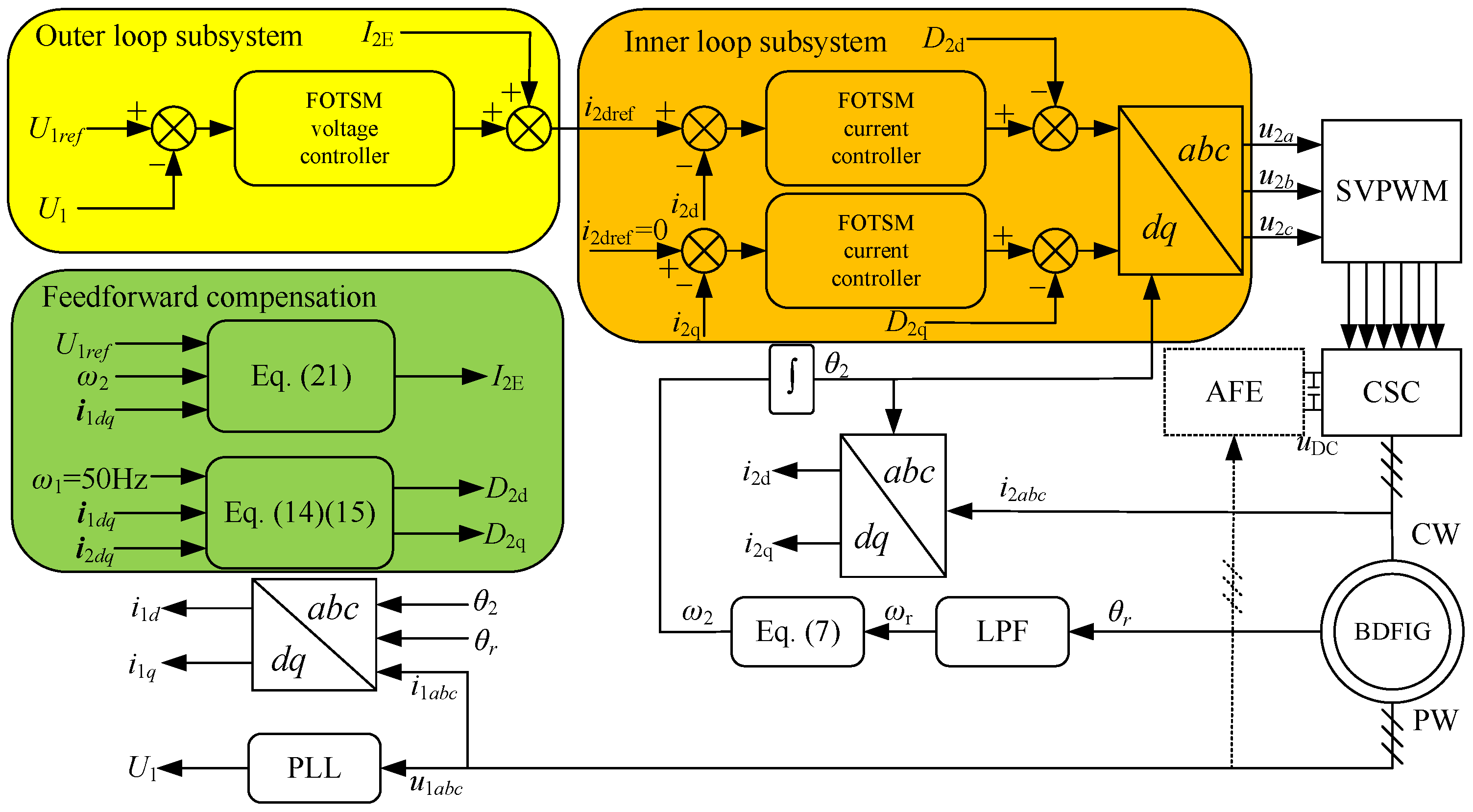
3. Full-Order Terminal Sliding-Mode Controller Design

Let $K_{u0}\mathrm{\Delta }{\dot{I}}_{2ref}=u_0$. A full-order terminal sliding manifold $s_0\in R^1$ is designed as

$$s_0=\dot{e_U}+c_0{e}_U^{q/p}$$

(39)

where $c_0$ is a constant, q and p are odds, and $0<q/p<1$.

Theorem 1.

Based on the sliding manifold (39) and the virtual control law as follows, the outer-loop voltage tracking error dynamics can be regulated to reach the presupposed manifold in finite time $t_{r0}\le (\left|s_0\left(0\right)\right|/{\eta }_0)$, thereafter remaining on it and converging to equilibrium point in finite time $t_{s0}\le p/[\left(c_0(p-q)\right){\left|e_U\left(t_{r0}\right)\right|}^{1-q/p}]$.

$$u_0=u_{0eq}+u_{0n}$$

(40)

$$u_{0eq}=c_0{e}_u^{q/p}$$

(41)

$$u_{0n}=\int k_0\mathrm{sgn}\left(s_0\right)\mathrm{d}\tau$$

(42)

$$k_0=\frac{M_{\delta }{M}_{deq}\left(t\right)+{\eta }_0}{1-M_{\delta }}$$

(43)

$$\mathrm{\Delta }{I}_{2ref}=\int \frac{1}{K_{u0}}{c}_0{e}_U^{q/p}+\frac{1}{K_{u0}}\int \int k_0\mathrm{sgn}\left(s_0\right)\mathrm{d}\tau \mathrm{d}\tau$$

(44)

where $M_{\delta }$ is defined in (34), $M_{deq}\left(t\right)$ is the upper bound of ${\dot{u}}_{0eq}$, and ${\eta }_0$ is a constant.

Proof of Theorem 1.

According to (30), Equation (39) can be rewritten as

$$\begin{array}{cc}\hfill s_0& =\dot{e_U}+c_0{e}_U^{q/p}\hfill \\ \hfill & =-K_{u0}\mathrm{\Delta }{\dot{I}}_{2ref}-\mathrm{\Delta }{K}_u\mathrm{\Delta }{\dot{I}}_{2ref}+K_{u0}{\ddot{e}}_{id}+c_0{e}_U^{q/p}\hfill \\ \hfill & =-u_0-{\delta }_U{u}_0+K_{u0}{\ddot{e}}_{id}+c_0{e}_U^{q/p}.\hfill \end{array}$$

(45)

A Lyapunov function is defined as $V_0=0.5s_0^2$, and the time derivative of $V_0$ is expressed as

$$\begin{array}{cc}\hfill {\dot{V}}_0& =s_0{\dot{s}}_0=-s_0{\dot{u}}_{0n}-s_0{\delta }_U{\dot{u}}_0+s_0{K}_{u0}{\ddot{e}}_{id}\hfill \\ \hfill & =-s_0{\dot{u}}_{0n}-s_0{\delta }_U{\dot{u}}_{0n}-s_0{\delta }_U{\dot{u}}_{0eq}+s_0{K}_{u0}{\ddot{e}}_{id}.\hfill \end{array}$$

(46)

Substituting the integral-type switching law (42) into the above equation gives

$$\begin{array}{cc}\hfill {\dot{V}}_0& \le -k_0\left|s_0\right|+k_0\left|s_0\right|\left|{\delta }_U\right|+\left|s_0\right|\left|{\delta }_U\right|\left|{\dot{u}}_{0eq}\right|+s_0{K}_{u0}{\ddot{e}}_{id}\hfill \\ \hfill & \le -k_0(1-M_{\delta })+M_{\delta }\left|s_0\right|\left|{\dot{u}}_{0eq}\right|+s_0{K}_{u0}{\ddot{e}}_{id}.\hfill \end{array}$$

(47)

Thus, ${\dot{V}}_0$ is satisfied:

$$\begin{array}{c}\hfill {\dot{V}}_0\le -∥s_0∥[(1-M_{\delta })k_0-M_{\delta }{M}_{d0eq}\left(t\right)],\end{array}$$

(48)

where $M_{deq}\left(t\right)$ is the upper bound of ${\dot{u}}_{eq}$. When $s_0\ne 0$, considering the switching gain (44) yields

$${\dot{V}}_0=s_0{\dot{s}}_0\le -{\eta }_0\left|s_0\right|+s_0{K}_{u0}{\ddot{e}}_{id}.$$

(49)

The inner loop tracking error $e_{id}$ and its derivative converge to zero in finite time and can be proven in the following Theorem 3. Then, we have

$${\dot{V}}_0\le -{\eta }_0\left|s_0\right|\le -\sqrt{2}{\eta }_0{V}_0^{1/2}<0.$$

(50)

According to the lemma of finite time convergence in [38], the above equation illustrates that the outer loop-error tracking error dynamics will reach the ideal sliding manifold within finite time under the designed virtual control law (40). It is maintained on the sliding mainfold $s_0=0$ thereafter. During the sliding motion, the error dynamics converge to zero in finite time. It is obvious that the virtual control law overcomes the ummatched uncertainties completely. This completes the proof. □

Let ${\mathit{e}}_i={\mathit{i}}_{ref}-\mathit{i}={[i_{dref}-i_d,0-i_q]}^T$ and ${\mathit{G}}_0{\mathit{u}}_{2dq}={\mathit{u}}_1$. With the subsystem (38), the error dynamics can be given as

$${\dot{\mathit{e}}}_i={\dot{\mathit{i}}}_{ref}-{\mathit{F}}_{00}{\mathit{i}}_{2dq}-{\mathit{u}}_1-\mathrm{\Delta }\mathit{G}{\mathit{G}}_0^{-1}{\mathit{u}}_1-{\rho }_1.$$

(51)

A full-order terminal sliding manifold $s_1\in R^2$ is designed as

$${\mathit{s}}_1=\dot{{\mathit{e}}_i}+{\mathit{C}}_1{\mathit{e}}_i^{q/p}$$

(52)

where ${\mathit{C}}_1=diag(c_{11},c_{12})$, $c_{11}>0$, $c_{12}>0$, and q and p are odds and $0<q/p<1$.

Theorem 2.

Based on the designed sliding surface (52), the virtual control law (40), and the following actual control law, the inner-loop current tracking error dynamics can be regulated to reach the sliding surface ${\mathit{s}}_1\left(t\right)=0$ in finite time $t_{r1}\le (∥{\mathit{s}}_1\left(0\right)∥/{\eta }_1)$. Then, the inner-loop tracking error ${\mathit{e}}_i$ and its derivative can converge to zero along the ideal sliding surface in finite time $t_{s1}\le max\{p/[\left(c_{11}(p-q)\right){\left|e_{id}\left(t_{r1d}\right)\right|}^{1-q/p}],p/[\left(c_{12}(p-q)\right){\left|e_{iq}\left(t_{r1q}\right)\right|}^{1-q/p}]\}$.

$${\mathit{u}}_1={\mathit{u}}_{1eq}+{\mathit{u}}_{1n}$$

(53)

$${\mathit{u}}_{1eq}=-{\mathit{F}}_{00}{\mathit{i}}_{2dq}+\frac{1}{K_{u0}}\left[\begin{array}{c}{c}_0{(-K_{u0}\mathrm{\Delta }{I}_{2ref})}^{q/p}+\int k_0\mathrm{sgn}\left(s_0\right)d\tau \\ 0\end{array}\right]$$

(54)

$${\mathit{u}}_{1n}=\int k_1\mathrm{sgn}\left({\mathit{s}}_0\right)d\tau$$

(55)

$$k_1=\frac{M_{\mathit{G}}{M}_{d1eq}\left(t\right)/T_{20}+c_{0}q{M}_{\delta }{M}_{\mathrm{\Delta }I2ref}^{(q-p)/p}{M}_{d\mathrm{\Delta }I2ref}/p+M_{d{\rho }_1}+{\eta }_1}{1-M_{\mathit{G}}/T_{20}}$$

(56)

$$\begin{array}{cc}\hfill {\mathit{u}}_{2dq}& ={\mathit{G}}_0^{-1}(-{\mathit{F}}_{00}{\mathit{i}}_{2dq}+\int k_1\mathrm{sgn}\left({\mathit{s}}_0\right)d\tau \hfill \\ \hfill & +\frac{1}{K_{u0}}\left[\begin{array}{c}{c}_0{(-K_{u0}\mathrm{\Delta }{I}_{2ref})}^{q/p}+\int k_0\mathrm{sgn}\left(s_0\right)d\tau \\ 0\end{array}\right])\hfill \end{array}$$

(57)

Proof of Theorem 2.

According to (51), the sliding manifold (52) can be rewritten as follows:

$${\mathit{s}}_1={\dot{\mathit{i}}}_{ref}-{\mathit{F}}_{00}{\mathit{i}}_{2dq}-{\mathit{u}}_1-\mathrm{\Delta }\mathit{G}{\mathit{G}}_0^{-1}{\mathit{u}}_1-{\rho }_1+{\mathit{C}}_1{\mathit{e}}_i^{q/p}.$$

(58)

Combined with (40), we have the following:

$${\mathit{s}}_1=\frac{1}{K_{u0}}\left[\begin{array}{c}{c}_0{e}_u^{q/p}+\int k_0\mathrm{sgn}\left(s_0\right)d\tau \\ 0\end{array}\right]-{\mathit{F}}_{00}{\mathit{i}}_{2dq}-{\mathit{u}}_1-\mathrm{\Delta }\mathit{G}{\mathit{G}}_0^{-1}{\mathit{u}}_1-{\rho }_1+{\mathit{C}}_1{\mathit{e}}_i^{q/p}.$$

(59)

Considering (30), the above can be rewritten as follows:

$$\begin{array}{cc}\hfill {\mathit{s}}_1& =\frac{1}{K_{u0}}\left[\begin{array}{c}{c}_0{(-K_{u0}\mathrm{\Delta }{I}_{2ref}-\mathrm{\Delta }{K}_u\mathrm{\Delta }{I}_{2ref})}^{q/p}+\int k_0\mathrm{sgn}\left(s_0\right)d\tau \\ 0\end{array}\right]\hfill \\ \hfill & -{\mathit{F}}_{00}{\mathit{i}}_{2dq}-{\mathit{u}}_1-\mathrm{\Delta }\mathit{G}{\mathit{G}}_0^{-1}{\mathit{u}}_1-{\rho }_1+{\mathit{C}}_1{\mathit{e}}_i^{q/p}.\hfill \end{array}$$

(60)

Substitute the actual control law (53) into the above, then we get

$$\begin{array}{cc}\hfill {\mathit{s}}_1& =\frac{1}{K_{u0}}\left[\begin{array}{c}{c}_0{(-\mathrm{\Delta }{K}_u\mathrm{\Delta }{I}_{2ref})}^{q/p}\\ 0\end{array}\right]-{\mathit{u}}_{1n}-\mathrm{\Delta }\mathit{G}{\mathit{G}}_0^{-1}{\mathit{u}}_1-{\rho }_1.\hfill \end{array}$$

(61)

Define a Lyapunov functionis as $V_1=0.5{\mathit{s}}_1^T{\mathit{s}}_1$, and the derivative of $V_1$ is expressed as

$$\begin{array}{cc}\hfill {\dot{V}}_1& ={\mathit{s}}_1^T{\dot{\mathit{s}}}_1\hfill \\ \hfill & =-{\mathit{s}}_1^T\dot{{\mathit{u}}_{1n}}-{\mathit{s}}_1^T\mathrm{\Delta }\mathit{G}{\mathit{G}}_0^{-1}{\dot{\mathit{u}}}_1-{\mathit{s}}_1^T{\dot{\rho }}_1+\frac{1}{K_{u0}}\left[\begin{array}{c}{c}_0(q/p){(-\mathrm{\Delta }{K}_u\mathrm{\Delta }{I}_{2ref})}^{(q-p)/p}{\dot{\mathrm{\Delta }I}}_{2ref}\\ 0\end{array}\right].\hfill \end{array}$$

(62)

Substituting (53) into the above gives

$$\begin{array}{cc}\hfill {\dot{V}}_1& =\frac{1}{K_{u0}}\left[\begin{array}{c}{c}_0(q/p){(-\mathrm{\Delta }{K}_u\mathrm{\Delta }{I}_{2ref})}^{(q-p)/p}\mathrm{\Delta }{\dot{I}}_{2ref}\\ 0\end{array}\right]\hfill \\ \hfill & -{\mathit{s}}_1^T\dot{{\mathit{u}}_{1n}}-{\mathit{s}}_1^T\mathrm{\Delta }\mathit{G}{\mathit{G}}_0^{-1}{\dot{\mathit{u}}}_{1n}-{\mathit{s}}_1^T\mathrm{\Delta }\mathit{G}{\mathit{G}}_0^{-1}{\dot{\mathit{u}}}_{1eq}-{\mathit{s}}_1^T{\dot{\rho }}_1.\hfill \end{array}$$

(63)

Thus,

$$\begin{array}{cc}\hfill {\dot{V}}_1& \le ∥{\mathit{s}}_1∥(-k_1+k_1∥\mathrm{\Delta }\mathit{G}∥∥{\mathit{G}}_0^{-1}∥+∥\mathrm{\Delta }\mathit{G}∥∥{\mathit{G}}_0^{-1}∥∥{\dot{\mathit{u}}}_{1eq}∥\hfill \\ \hfill & +\frac{c_{0}q}{p}∥{\delta }_U∥∥\mathrm{\Delta }{I}_{2ref}^{(q-p)/p}∥∥\mathrm{\Delta }{\dot{I}}_{2ref}∥+∥{\dot{\rho }}_1∥).\hfill \end{array}$$

(64)

From the above, the upper bound of the actual control law can be estimated as

$$∥{\dot{\mathit{u}}}_1∥\le ∥{\dot{\mathit{u}}}_{1eq}∥+∥{\dot{\mathit{u}}}_{1n}∥\le \sqrt{2}{k}_1+M_{d1eq}\left(t\right).$$

(65)

According to (44), the upper bound of $\mathrm{\Delta }{I}_{2ref}$ and its derivative are estimated as

$$\begin{array}{c}\hfill \mathrm{\Delta }{I}_{2ref}=\int \frac{1}{K_{u0}}{c}_0{e}_u^{q/p}+\frac{1}{K_{u0}}\int \int k_0\mathrm{sgn}\left(s_0\right)d\tau \le M_{\mathrm{\Delta }I2ref}\\ \hfill \mathrm{\Delta }{\dot{I}}_{2ref}=\frac{1}{K_{u0}}{c}_0{e}_u^{q/p}+\frac{1}{K_{u0}}\int k_0\mathrm{sgn}\left(s_0\right)d\tau \le M_{d\mathrm{\Delta }I2ref}.\end{array}$$

(66)

Combined with adaptive switching gain (56), when $V_1\ne 0$

$$\begin{array}{cc}\hfill {\dot{V}}_1& \le ∥{\mathit{s}}_1∥\left[\begin{array}{c}\hfill -k_1(1-M_{\mathit{G}}/T_{20})+M_{\mathit{G}}{M}_{d1eq}\left(t\right)/T_{20}\\ \hfill +c_{0}q{M}_{\delta }{M}_{\mathrm{\Delta }I2ref}^{(q-p)/p}{M}_{d\mathrm{\Delta }I2ref}/p+M_{d{\rho }_1}\end{array}\right]\hfill \\ \hfill & \le -\sqrt{2}{\eta }_1{V}_1^{1/2}.\hfill \end{array}$$

(67)

Similar to the proof of Theorem 1, the above equation means that the error dynamic approaches the ideal sliding surface ${\mathit{s}}_1=0$ in finite time. Additionally, the tracking errors of CW current and its derivative converge to the equilibrium point in finite time. From Theorem 1, $e_U$ can converge to zero in finite time. This complete the proof. □

According to Theroems 1 and 2, the PW voltage controller is designed for the outer-loop and the CW current vector controllers are utilized for the inner-loop. The block diagram of the control scheme of the BDFIG as shown in Figure 2. The phase-locked loop (PLL) is used to track the amplitude of the output voltage, which is omitted here for space due to its simplicity.

4. Simulations

In order to demonstrate the effectiveness of the proposed method, PI controllers, linear sliding mode (LSM), and FOTSM controllers are designed for performance comparison. The parameters of the BDFIG are listed in

Table 1. The parameters of the BDFIG.

Symbol	Mean	Value
$S_e$	Capacity	30 kVA
${\omega }_e$	Speed range	600–1200 rpm
$p_1,p_2$	PW and CW pole pairs	1, 3
$U_{1e},I_{1e}$	PW rate voltage and current	380 V, 45 A
$U_{2e},I_{2e}$	CW rate voltage and current	0–350 V, 0–50 A
$R_1$	PW resistances	$0.4034\mathrm{\Omega }$
$R_2$	CW resistances	$0.2608\mathrm{\Omega }$
$R_r$	Rotor resistances	$0.3339\mathrm{\Omega }$
$L_1$	PW inductances	474.9 mH
$L_2$	CW inductances	32.16 mH
$L_r$	rotor inductances	225.2 mH
$L_{1r}$	Mutual inductance between PW and rotor	306.9 mH
$L_{2r}$	Mutual inductance between CW and rotor	25.84 mH

, and the controllers design parameters in

Table 2. Controller design parameters.

Control	Outer Loop Controller Parameters	Inner Loop Controller Parameters
PI	$K_p=0.07,K_i=18$	$K_p=21.5,K_i=972$
LSM	$c=300,k=1000$	$K_p=21.5,K_i=972$
FOTSM	$c_0=300,k_0=4000,q/p=3/5$	$c_{11}=c_{12}=1000,k_1=6000,q/p=3/5$

.

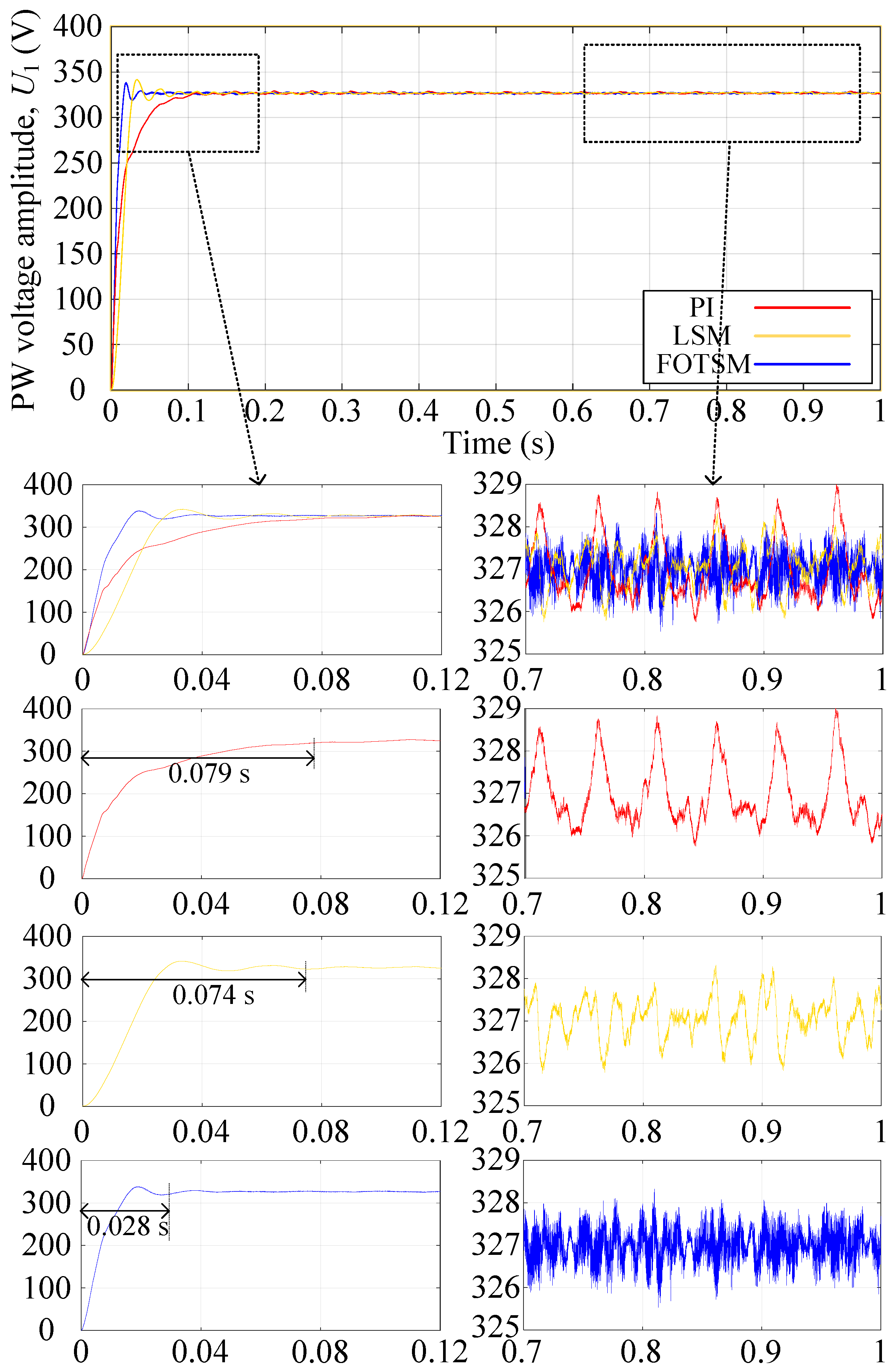
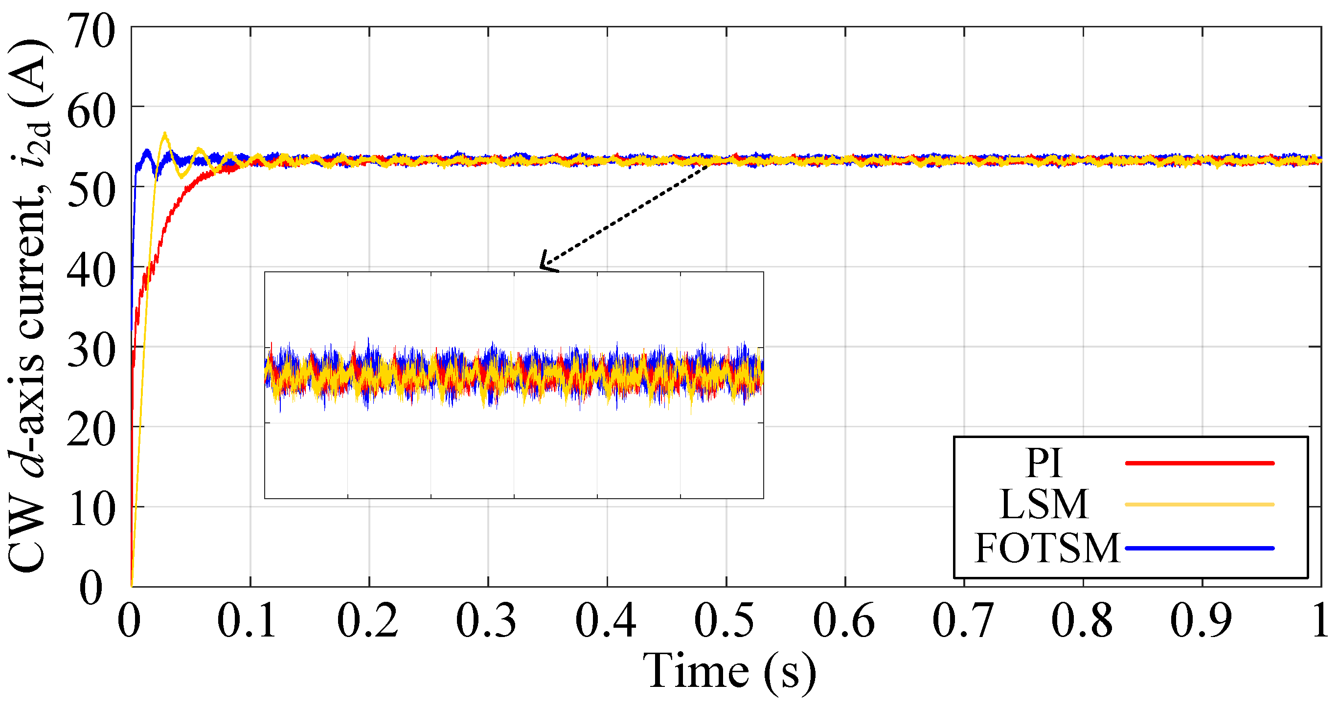
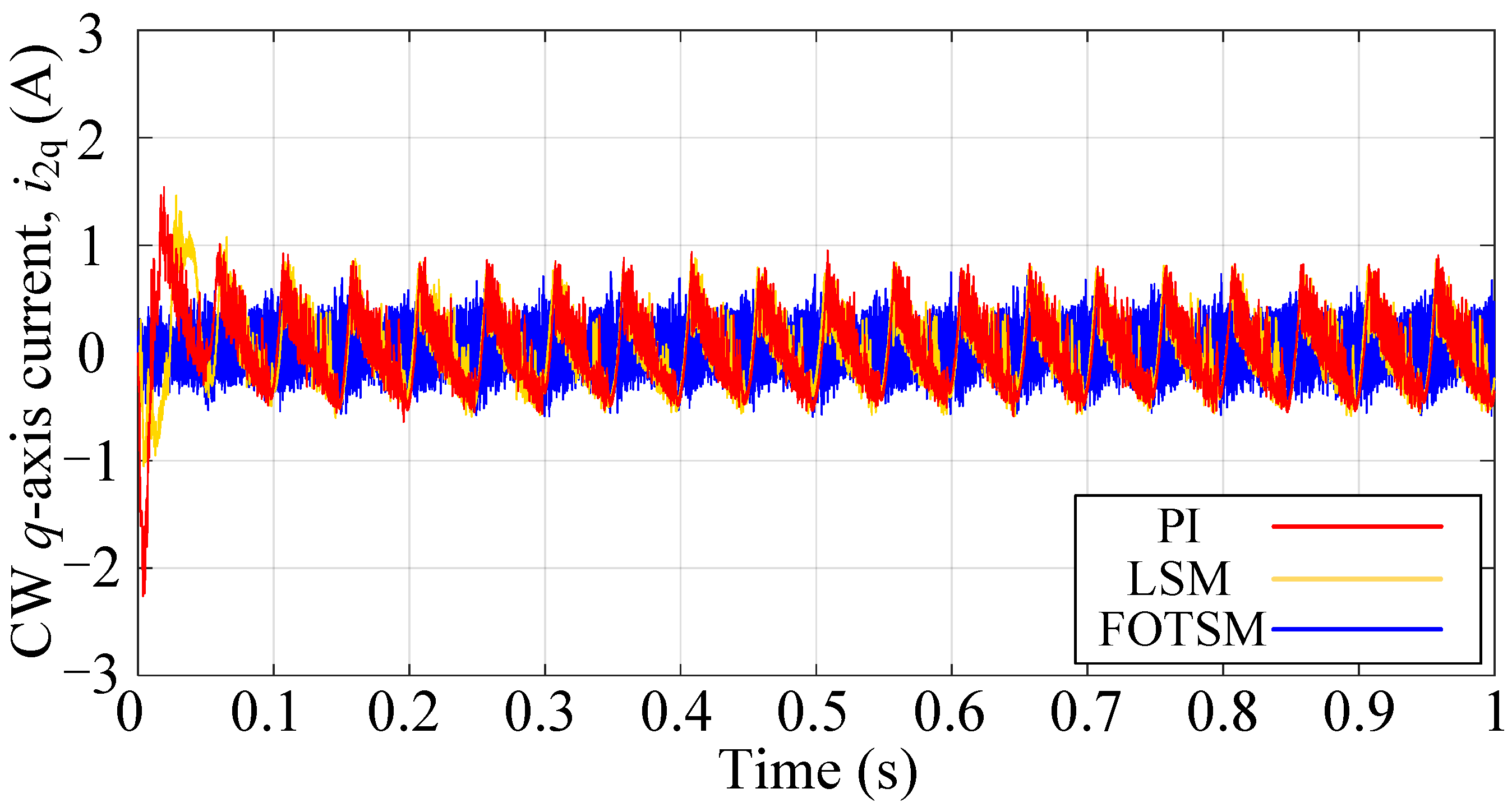
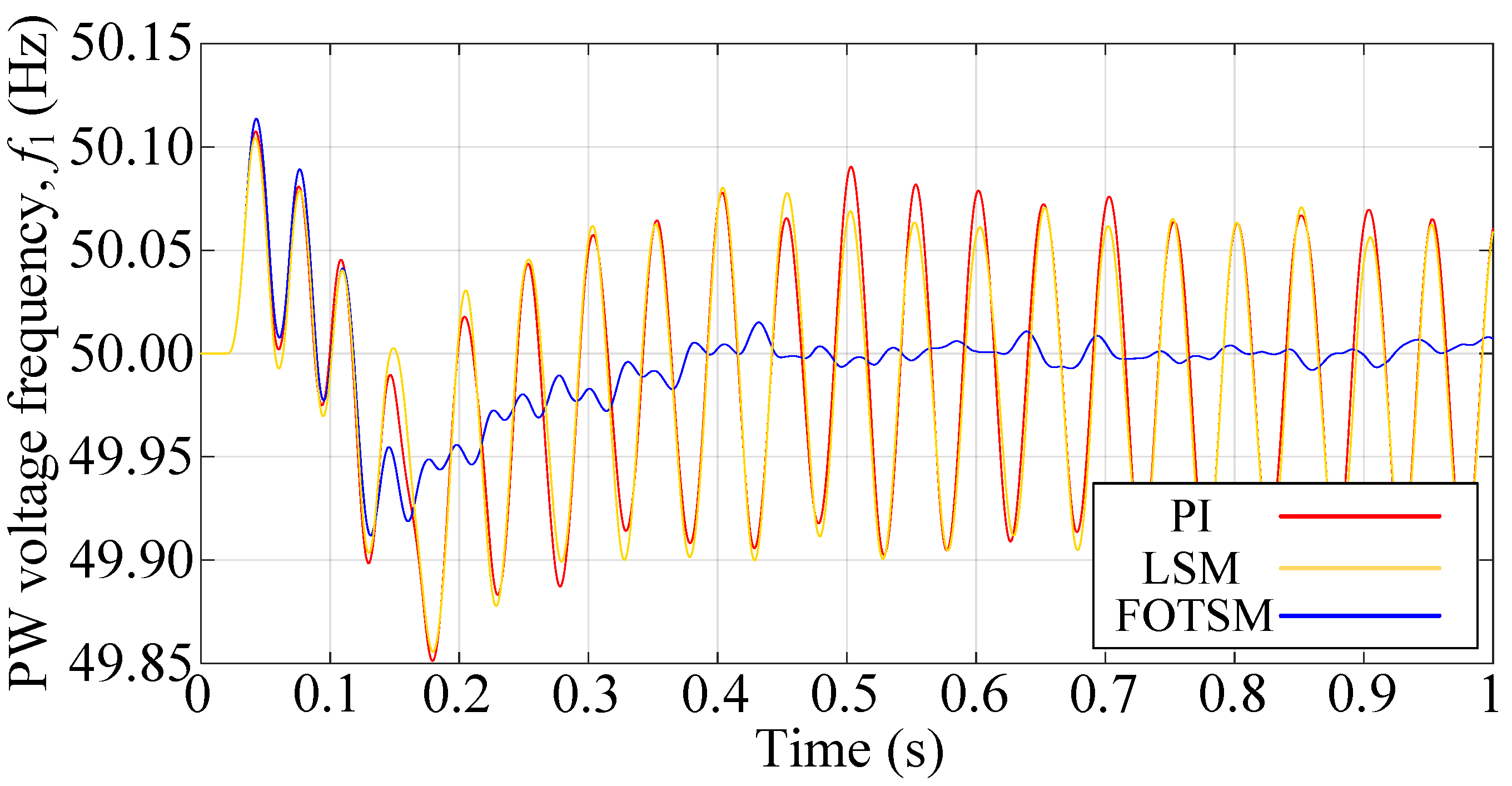
4.1. Start-Up Response

The BDFIG starts at 0s and runs for 1.0 s in total. The speed of the prime mover is set as 700 rpm in the simulations. In order to characterize the parameter mismatch caused by the change in temperature and frequency, the resistances and inductances are set as $105\%$ of the real values in the simulations. The reference frequency and amplitude of the PW voltage are 50 Hz and 327 V, respectively. The load is a balance three-phase resistive load with resistances of $25\Omega$ for each phase. The PI, LSM, and the proposed FOTSM controllers during the voltage start-up process are shown in Figure 3. It can be seen that the settling time of the voltage response under PI, LSM, and FOTSM are $0.079$ s, $0.074$ s, and $0.028$ s, respectively. The BDFIG under the proposed FOTSM controller has a better dynamic response. It is obvious that the accuracy of the voltage response is enhanced and that the ripple is reduced. Figure 4 shows that the d-axis current response under the FOTSM can approach the given current faster than the PI and the LSM. It is evident that the ripple of q-axis current under the FOTSM is smaller than PI and LSM in Figure 5 owing to the integral-type control law and the adaptive switching gain. In Figure 6, the frequency under the PI and the LSM has a larger ripple than that under the FOTSM.

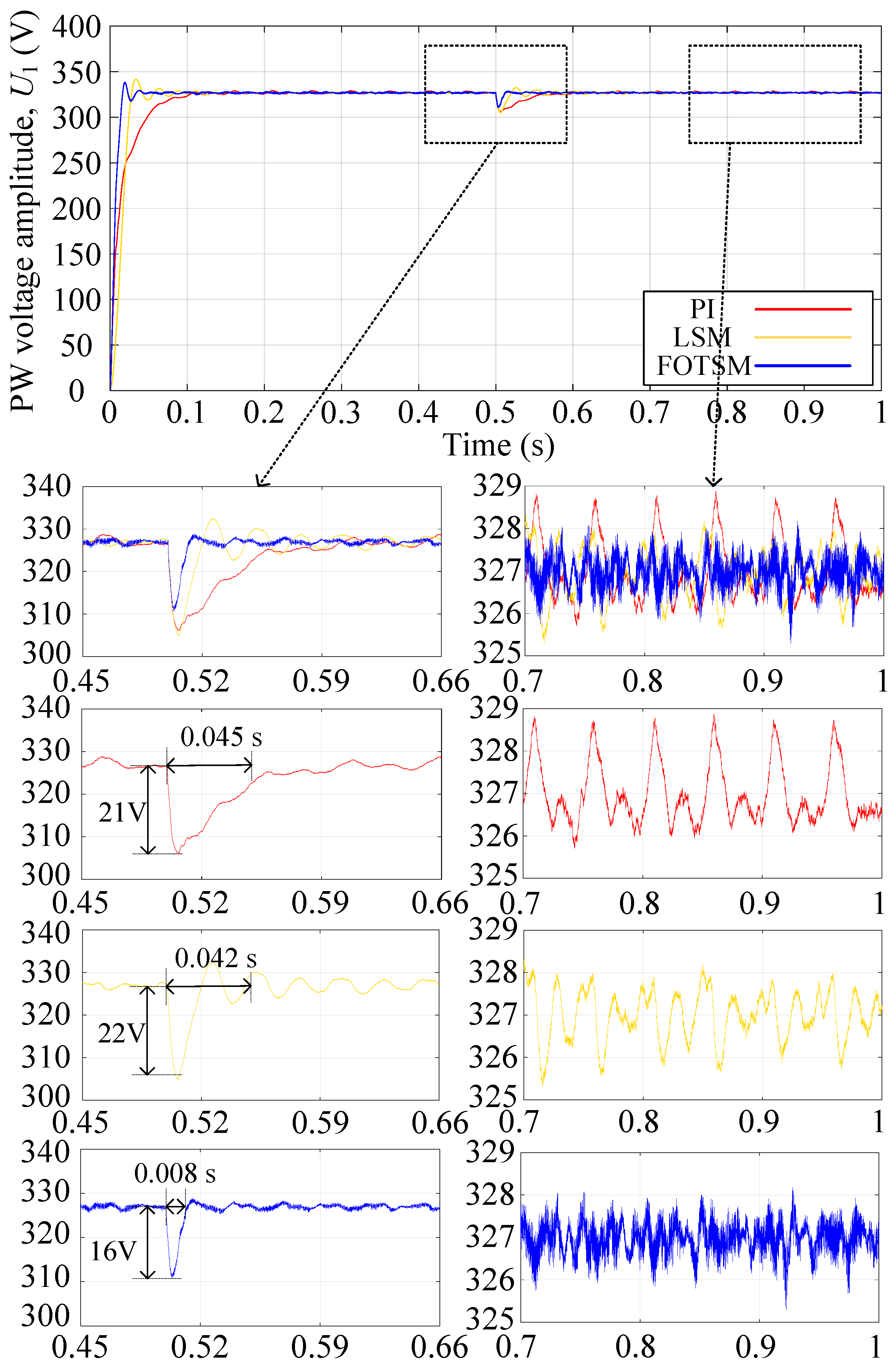
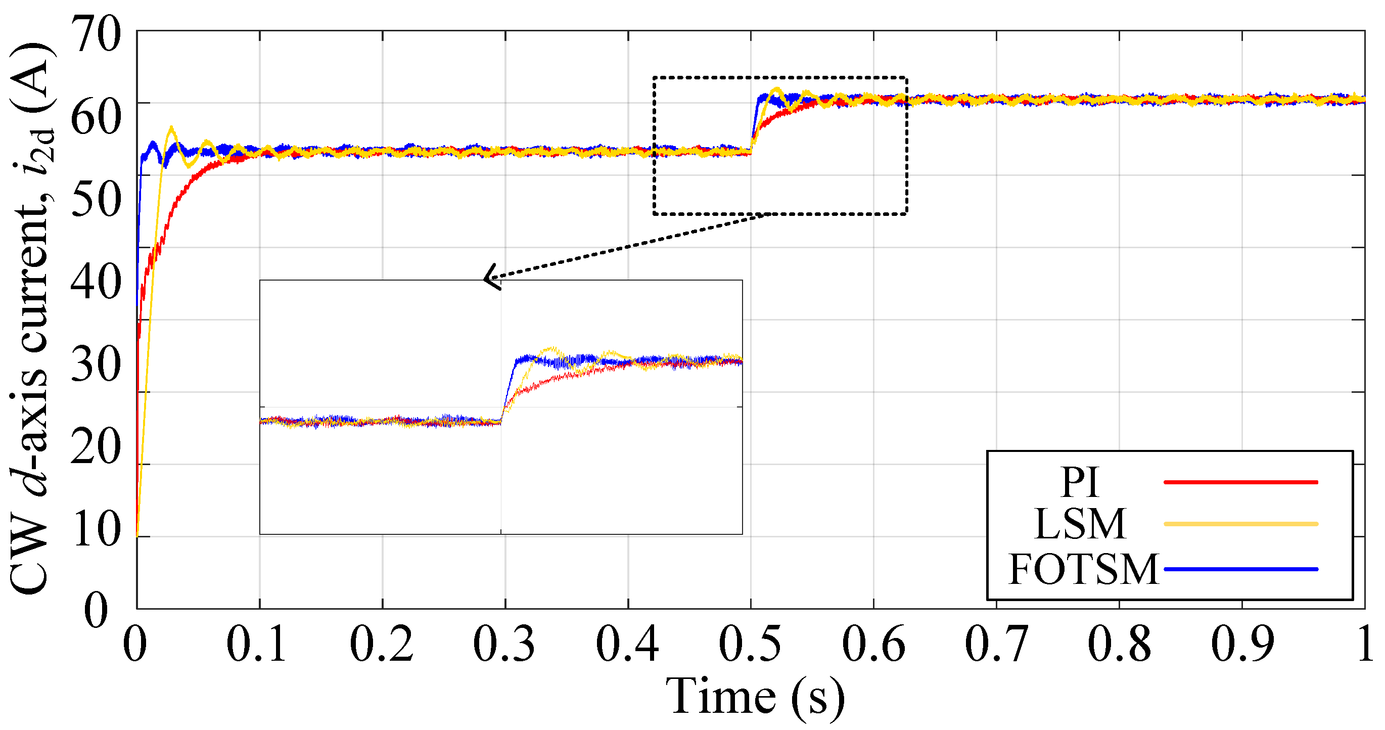
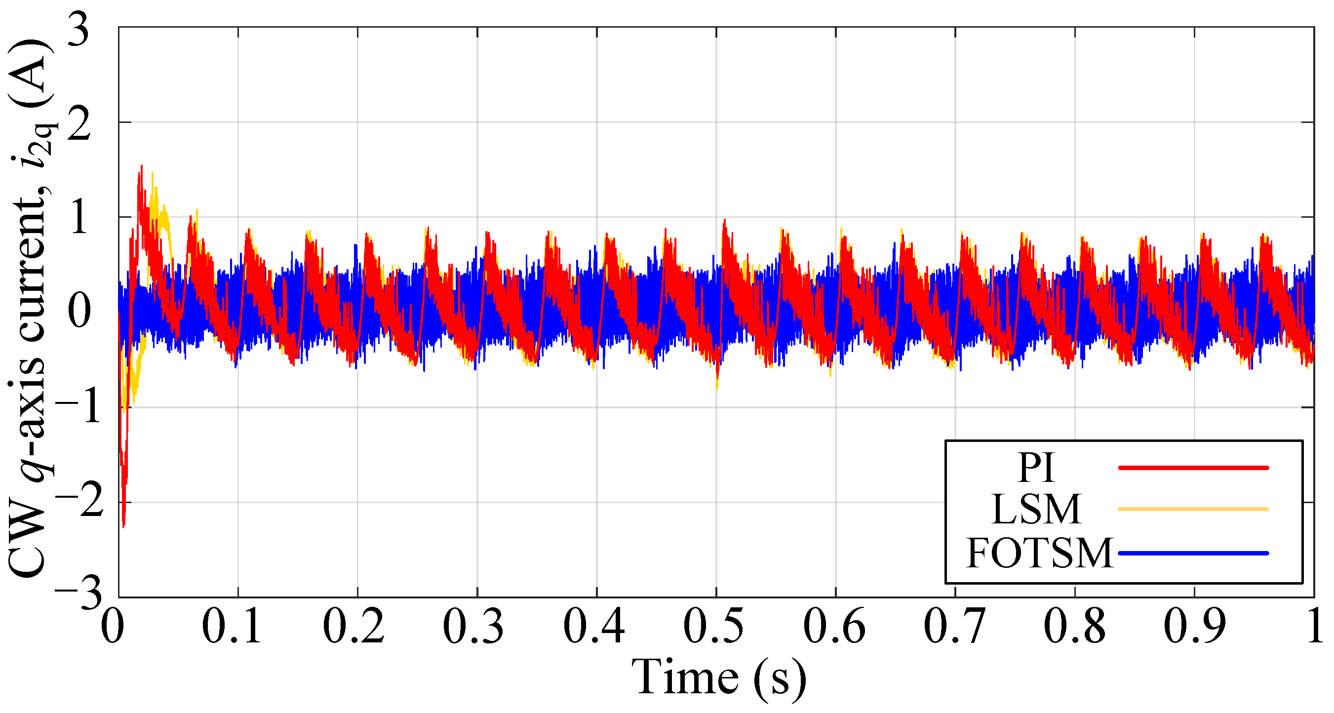
4.2. Load Adding Response

In order to attest to the robustness of the three control methods, another balance three-phase resistive load with resistances of $120\mathrm{\Omega }$ for each phase is added to the system in $0.5$ s. The condition of the simulations is the same as the start-up response and the simulation results are shown in Figure 7, Figure 8, Figure 9 and Figure 10. According to the simulation results shown in Figure 8 that the voltage amplitude drops under the PI, the LSM and the FOTSM are 21 V, 22 V, and 16 V, respectively. In addition, the settling time of the voltage response under the PI, the LSM, and the FOTSM are $0.045$ s, $0.042$ s, and $0.008$ s, respectively, which means that the proposed FOTSM has a faster dynamic response and stronger robustness. It is obvious that the tracking error of the PW voltage amplitude under FOTSM is still smaller than the PI and the LSM when the load is added. In Figure 8, the current response under the FOTSM can converge to the equilibrium point faster than the PI and the LSM when the load is added. It can be seen from Figure 9 that the ripple of the q-axis current under the FOTSM is smaller than those under the PI and the LSM. In Figure 10, the fluctuation of frequency under the PI, the LSM, and the FOTSM is similar when the balance three-phase resistive load is added. However, the FOTSM has a faster recovery time and smaller ripple in steady-state than that under the PI and the LSM. These results further verify that the proposed FOTSM has a better robustness against the uncertainties.

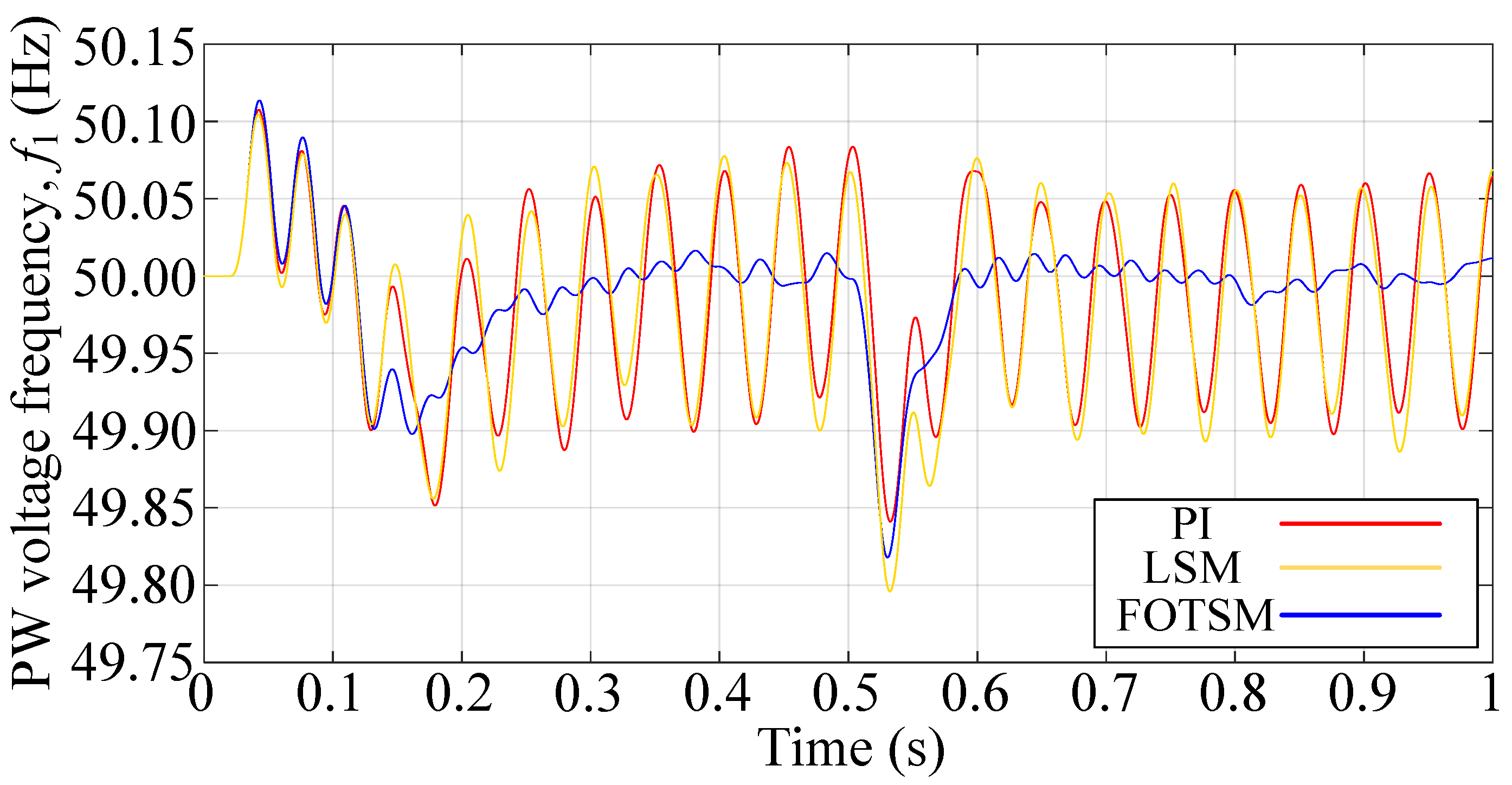
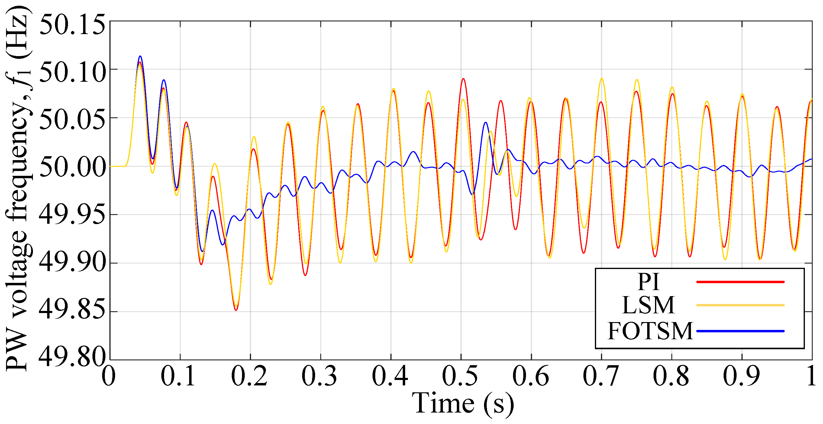
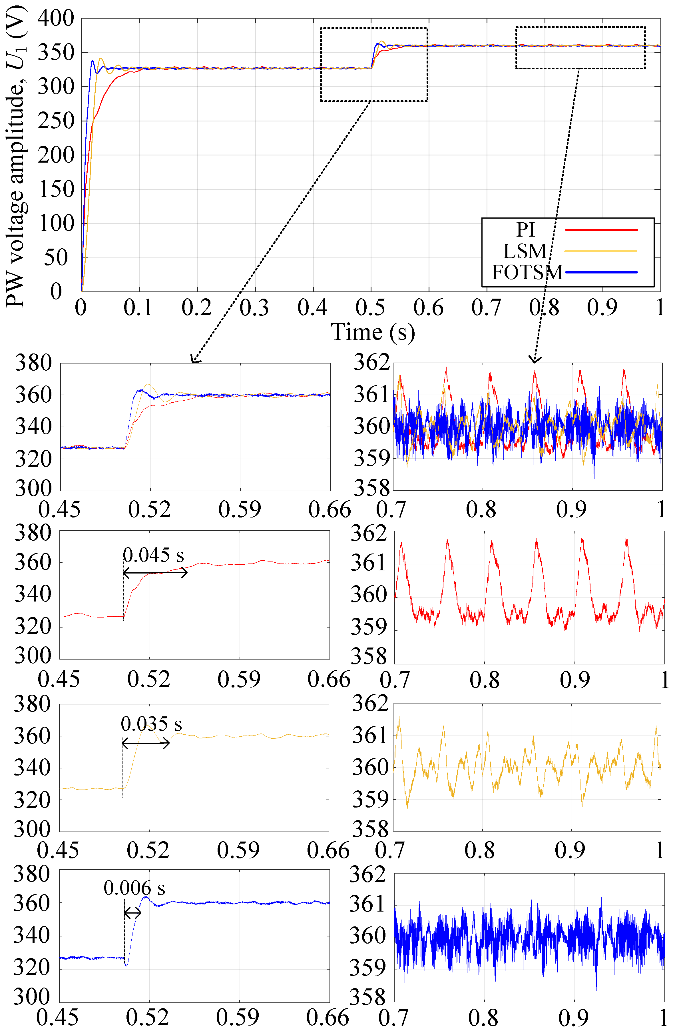
4.3. Voltage Change Response

In order to demonstrate the dynamic response of the BDFIG using the FOTSM controllers. The reference of output PW-voltage amplitude is changed from 327 V to 360 V at $0.5$ s. The condition of the simulations is the same as the start-up response and the simulation results are shown in Figure 11, Figure 12, Figure 13 and Figure 14. It can be concluded from Figure 11 that the settling time of the voltage response under the PI, the LSM, and the FOTSM are $0.045$ s, $0.035$ s, and $0.006$ s, respectively, when the reference of voltage amplitude is changed from 327 V to 360 V at $0.5$ s. Meanwhile, the precision of the output voltage under the FOTSM is better than those under the PI and the LSM. Figure 12 shows the d-axis current response under PI-, LSM-, and FOTSM- controllers, which verifies that the proposed method has a fast dynamic response. It is obvious from Figure 13 that the q-axis current response has a smaller ripple than those under the PI and the LSM. In Figure 14, the frequency of PW voltage response under the FOTSM has better precision and smaller fluctuation than the PI and the LSM in the condition of voltage change. Therefore, it can be concluded that the proposed FOTSM controllers have advantages in dynamic response and robustness against the uncertainties caused by parameter perturbation.

5. Discussion

For the implementation of high-performance BDFIG-based islanded microgrids, a sensorless control method, a harmonic elimination method, an adaptive gain to reduce the complexity of the control gain design, and an experimental study of the proposed control method will be our future work.

6. Conclusions

In this paper, a novel FOTSM control method was proposed to enhance the accuracy, the rapidness, and the robustness of the BDFIG-based islanded microgrids and to improve the output voltage quality. Different from the existing control methods, all of the matched and mismatched uncertainties in the BDFIG system are fully considered. With the use of the virtual control technique-based FOTSM, the tracking errors can be forced to converge to zero in finite time, and the matched and mismatched uncertainties can be thoroughly compensated, which improve the disturbance rejection capability of the BDFIG system. Owing to the integral control law with the adaptive gain, the output signals of the proposed controllers are smooth. Comprehensive simulation results have proved the effectiveness and feasibility of the proposed method in this work.

References

1. Zeng, Y.; Cheng, M.; Wei, X.; Zhang, G. Grid-Connected and Standalone Control for Dual-Stator Brushless Doubly Fed Induction Generator. IEEE Trans. Ind. Electron. 2021, 10, 9196–9206. [Google Scholar] [CrossRef]
2. Xu, W.; Hussien, M.; Liu, Y.; Islam, M.; Allam, S. Sensorless Voltage Control Schemes for Brushless Doubly-Fed Induction Generators in Stand-Alone and Grid-Connected Applications. IEEE Trans. Energy Convers. 2020, 35, 1781–1795. [Google Scholar] [CrossRef]
3. Sami, I.; Ullah, S.; Ali, Z.; Ullah, N.; Ro, J.-S. A Super Twisting Fractional Order Terminal Sliding Mode Control for DFIG-Based Wind Energy Conversion System. Energies 2020, 13, 2158. [Google Scholar] [CrossRef]
4. Min, L.; Chen, Y.; Debin, Z.; Jingyuan, S.; Yong, K. Virtual Synchronous Control Based on Control Winding Orientation for Brushless Doubly Fed Induction Generator (BDFIG) Wind Turbines Under Symmetrical Grid Faults. Energies 2019, 12, 319. [Google Scholar]
5. Taluo, T.; Ristić, L.; Jovanović, M. Dynamic Modeling and Control of BDFRG under Unbalanced Grid Conditions. Energies 2021, 14, 4297. [Google Scholar] [CrossRef]
6. Xu, W.; Elbabo, M.; Omer, M.; Liu, Y.; Islam, M.R. Negative Sequence Voltage Compensating for Unbalanced Standalone Brushless Doubly-Fed Induction Generator. IEEE Trans. Power Electron. 2020, 35, 667–680. [Google Scholar] [CrossRef]
7. Ullah, N.; Sami, I.; Chowdhury, M.; Techato, K.; Alkhammash, H. Artificial Intelligence Integrated Fractional Order Control of Doubly Fed Induction Generator-Based Wind Energy System. IEEE Access 2021, 9, 5734–5748. [Google Scholar] [CrossRef]
8. Han, P.; Cheng, M.; Jiang, Y.l.; Chen, Z. Torque/Power Density Optimization of a Dual-Stator Brushless Doubly-Fed Induction Generator for Wind Power Application. IEEE Trans. Ind. Electron. 2017, 64, 9864–9875. [Google Scholar] [CrossRef]
9. Barati, F.; McMahon, R.; Shao, S.Y.; Abdi, E.; Oraee, H. Generalized Vector Control for Brushless Doubly Fed Machines with Nested-Loop Rotor. IEEE Trans. Ind. Electron. 2013, 60, 2477–2485. [Google Scholar] [CrossRef]
10. Izaskun, S.; Javier, P.; Miguel, A.R.; Gonzalo, A. Direct torque control design and experimental evaluation for the brushless doubly fed machine. Energy Convers. Manag. 2011, 52, 142–149. [Google Scholar]
11. Shao, S.Y.; Abdi, E.; McMahon, R. Low-Cost Variable Speed Drive Based on a Brushless Doubly-Fed Motor and a Fractional Unidirectional Converter. IEEE Trans. Ind. Electron. 2008, 59, 317–325. [Google Scholar] [CrossRef]
12. Zhang, A.; Wang, X.; Jia, W.X.; Ma, Y. Indirect Stator-Quantities Control for the Brushless Doubly Fed Induction Machine. IEEE Trans. Power Electron. 2014, 29, 1392–1401. [Google Scholar] [CrossRef]
13. Sebtahmadi, S.S.; Pirasteh, H.; Aghay Kaboli, S.H.; Radan, A.; Mekhilef, S. A 12-Sector Space Vector Switching Scheme for Performance Improvement of Matrix-Converter-Based DTC of IM Drive. IEEE Trans. Power Electron. 2015, 30, 3804–3817. [Google Scholar] [CrossRef]
14. Liu, Y.; Xu, W.; Zhu, J.G.; Blaabjerg, F. Sensorless Control of Standalone Brushless Doubly Fed Induction Generator Feeding Unbalanced Loads in a Ship Shaft Power Generation System. IEEE Trans. Ind. Electron. 2019, 66, 739–749. [Google Scholar] [CrossRef]
15. Lu, X.; Lai, J.; Liu, G. Master-Slave Cooperation for Multi-DC-MGs via Variable Cyber Networks. IEEE Trans. Cybern. 2021. [Google Scholar] [CrossRef]
16. Vargas, U.; Ramirez, A. Extended Harmonic Domain Model of a Wind Turbine Generator for Harmonic Transient Analysis. IEEE Trans. Power Deliv. 2016, 31, 1360–1368. [Google Scholar] [CrossRef]
17. Kim, J.; Seok, J.K.; Muljadi, E.; Kang, Y. Adaptive Q-V Scheme for the Voltage Control of a DFIG-Based Wind Power Plant. IEEE Trans. Power Electron. 2016, 31, 3586–3599. [Google Scholar] [CrossRef]
18. Qin, B.; Sun, H.; Ma, J.; Li, W.; Ding, T.; Wang, Z.; Zomaya, A.Y. Robust H∞ Control of Doubly Fed Wind Generator via State-Dependent Riccati Equation Technique. IEEE Trans. Power Syst. 2021, 34, 2390–2400. [Google Scholar] [CrossRef]
19. Sharmila, V.; Rakkiyappan, R.; Joo, Y.H. Fuzzy Sampled-Data Control for DFIG-Based Wind Turbine with Stochastic Actuator Failures. IEEE Trans. Syst. Man Cybern. Syst. 2021, 51, 2199–2211. [Google Scholar] [CrossRef]
20. Lu, L.; Avila, N.F.; Chu, C.C.; Yeh, T.W. Model Reference Adaptive Back-Electromotive-Force Estimators for Sensorless Control of Grid-Connected DFIGs. IEEE Trans. Ind. Appl. 2018, 54, 1701–1711. [Google Scholar] [CrossRef]
21. Errouissi, R.; Al-Durra, A.; Muyeen, S.M.; Leng, S.Y.; Blaabjerg, F. Offset-Free Direct Power Control of DFIG Under Continuous-Time Model Predictive Control. IEEE Trans. Power Electron. 2017, 32, 2265–2277. [Google Scholar] [CrossRef]
22. Tohidi, A.; Hajieghrary, H.; Hsieh, M.A. Adaptive Disturbance Rejection Control Scheme for DFIG-Based Wind Turbine: Theory and Experiments. IEEE Trans. Ind. Appl. 2016, 52, 2006–2015. [Google Scholar] [CrossRef]
23. Lu, X.; Lai, J. Communication Constraints for Distributed Secondary Control of Heterogenous Microgrids: A Survey. IEEE Trans. Ind. Appl. 2021. [Google Scholar] [CrossRef]
24. Lai, J.; Lu, X.; Dong, Z.; Cheng, S. Resilient Distributed Multiagent Control for AC Microgrid Networks Subject to Disturbances. IEEE Trans. Syst. Man Cybern. Syst. 2021. [Google Scholar] [CrossRef]
25. Ruiz-Cruz, R.; Sanchez, E.N.; Loukianov, A.G.; Ruz-Hernandez, J.A. Real-Time Neural Inverse Optimal Control for a Wind Generator. IEEE Trans. Sustain. Energy 2019, 10, 1172–1183. [Google Scholar] [CrossRef]
26. Hu, J.; He, N.; Hu, B.; He, Y.; Zhu, Z. Direct Active and Reactive Power Regulation of DFIG Using Sliding-Mode Control Approach. IEEE Trans. Energy Convers. 2010, 25, 1028–1039. [Google Scholar] [CrossRef]
27. Lascu, C.; Boldea, I.; Blaabjerg, F. Direct torque control of sensorless induction motor drives: A sliding-mode approach. IEEE Trans. Ind. Appl. 2004, 40, 582–590. [Google Scholar] [CrossRef]
28. Zhou, M.; Cheng, S.; Feng, Y.; Xu, W.; Wang, L.; Cai, W. Full-Order Terminal Sliding-Mode based Sensorless Control of Induction Motor with Gain Adaptation. IEEE J. Emerg. Sel. Top. Power Electron. 2021. [Google Scholar] [CrossRef]
29. Sun, D.; Wang, X.; Nian, H.; Zhu, Z. A Sliding-Mode Direct Power Control Strategy for DFIG Under Both Balanced and Unbalanced Grid Conditions Using Extended Active Power. IEEE Trans. Power Electron. 2018, 33, 1313–1322. [Google Scholar] [CrossRef]
30. Sadeghi, R.; Madani, S.M.; Ataei, M.; Agha Kashkooli, M.R.; Ademi, S. Super-Twisting Sliding Mode Direct Power Control of a Brushless Doubly Fed Induction Generator. IEEE Trans. Ind. Electron. 2018, 65, 9147–9156. [Google Scholar] [CrossRef]
31. Amin, I.K.; Uddin, M.N. Nonlinear Control Operation of DFIG-Based WECS Incorporated With Machine Loss Reduction Scheme. IEEE Trans. Power Electron. 2020, 35, 7031–7044. [Google Scholar] [CrossRef]
32. Chen, S.; Cheung, N.C.; Wong, K.C.; Wu, J. Integral Sliding-Mode Direct Torque Control of Doubly-Fed Induction Generators Under Unbalanced Grid Voltage. IEEE Trans. Energy Convers. 2010, 25, 356–368. [Google Scholar] [CrossRef]
33. Evangelista, C.; Valenciaga, F.; Puleston, P. Active and Reactive Power Control for Wind Turbine Based on a MIMO 2-Sliding Mode Algorithm with Variable Gains. IEEE Trans. Energy Convers. 2013, 28, 682–689. [Google Scholar] [CrossRef]
34. Evangelista, C.A.; Pisano, A.; Puleston, P.; Usai, E. Receding Horizon Adaptive Second-Order Sliding Mode Control for Doubly-Fed Induction Generator Based Wind Turbine. IEEE Trans. Control Syst. Technol. 2016, 25, 73–84. [Google Scholar] [CrossRef]
35. Yan, X.; Cheng, M.; Xu, L.; Zeng, Y. Dual-Objective Control Using an SMC-Based CW Current Controller for Cascaded Brushless Doubly Fed Induction Generator. IEEE Trans. Ind. Appl. 2020, 56, 7109–7120. [Google Scholar] [CrossRef]
36. Zhang, G.; Yang, J.; Sun, Y.; Su, M.; Tang, W.; Zhu, Q.; Wang, H. A Robust Control Scheme Based on ISMC for the Brushless Doubly Fed Induction Machine. IEEE Trans. Power Electron. 2018, 33, 3129–3140. [Google Scholar] [CrossRef]
37. Yu, X.; Feng, Y.; Man, Z. Terminal Sliding Mode Control—An Overview. IEEE Open J. Ind. Electron. Soc. 2021, 2, 36–52. [Google Scholar] [CrossRef]
38. Feng, Y.; Zhou, M.; Zheng, X.; Han, F.; Yu, X. Full-order terminal sliding-mode control of MIMO systems with unmatched uncertainties. J. Frankl. Inst. 2017, 1, 1–22. [Google Scholar] [CrossRef]
Figure 1. The structure of the BDFIG in the ship power mircogrid, where the SCS means the CW-side converter and the AFE means the active front end.
Energies 14 07302 g001
Figure 2. Block diagram of the control scheme of the standalone BDFIG.
Energies 14 07302 g002
Figure 3. The PW-voltage amplitude responses under PI, LSM, and FOTSM during the start-up process.
Energies 14 07302 g003
Figure 4. The CW d-axis current responses under PI, LSM, and FOTSM during the start-up process.
Energies 14 07302 g004
Figure 5. The CW q-axis current responses under PI, LSM, and FOTSM during the start-up process.
Energies 14 07302 g005
Figure 6. The PW voltage frequency responses under PI, LSM, and FOTSM during the start-up process.
Energies 14 07302 g006
Figure 7. The PW-voltage amplitude responses under PI, LSM, and FOTSM during the load adding process.
Energies 14 07302 g007
Figure 8. The CW d-axis current responses under PI, LSM, and FOTSM during the load adding process.
Energies 14 07302 g008
Figure 9. The CW q-axis current responses under PI, LSM, and FOTSM during the load adding process.
Energies 14 07302 g009
Figure 10. The PW voltage frequency responses under PI, LSM, and FOTSM during the load adding process.
Energies 14 07302 g010
Figure 11. The PW-voltage amplitude responses under PI, LSM, and FOTSM during the voltage change process.
Energies 14 07302 g011
Figure 12. The CW d-axis current responses under PI, LSM, and FOTSM during the voltage change process.
Energies 14 07302 g012
Figure 13. The CW q-axis current responses under PI, LSM, and FOTSM during the voltage change process.
Energies 14 07302 g013
Figure 14. The PW voltage frequency responses under PI, LSM, and FOTSM during the voltage change process.
Energies 14 07302 g014