Abstract
Bioenergy with carbon capture and storage (BECCS) can sequester atmospheric CO2, while producing electricity. The CO2 avoidance cost (CAC) is used to calculate the marginal cost of avoided CO2 emissions for BECCS as compared to other established energy technologies. A comparative analysis using four different reference-case power plants for CAC calculations is performed here to evaluate the CO2 avoidance cost of BECCS implementation. Results from this work demonstrate that BECCS can generate electricity at costs competitive with other neutral emissions technologies, while simultaneously removing CO2 from the atmosphere. Approximately 73% of current coal power plants are approaching retirement by the year 2035 in the U.S. After considering CO2 sequestered from the atmosphere and coal power plant CO2 emissions displaced by BECCS, CO2 emissions can be reduced by 1.4 billion tonnes per year in the U.S. alone at a cost of $88 to $116 per tonne of CO2 removed from the atmosphere, for 10% to 90% of available biomass used, respectively. CAC calculations in this paper indicate that BECCS can help the U.S. and other countries transition to a decarbonized electricity grid, as simulations presented in this paper predict that BECCS power plants operate at lower CACs than coal plants with CCS.
1. Introduction
Currently, almost all forms of anthropogenic activity contribute to greenhouse gas (GHG) emissions [1,2]. According to the U.S. Environmental Protection Agency (EPA), the largest source of GHG emissions from human activities in the U.S. is the burning of fossil fuels for energy including electricity, heat, and transportation [3,4]. The U.S. Energy Information Agency (EIA) estimates that the U.S. emitted roughly 5.1 billion tonnes of energy-related CO2 in 2017, while the global energy-related CO2 emissions totaled roughly 32.5 billion tonnes [4]. Transportation was estimated to be the largest share of CO2 emissions in the U.S., with a share of roughly 28.2% in 2018 [4]. These emissions emerge from the burning of fossil fuels to power transportation vehicles, such as automobiles, airplanes, and ships. Additionally, most of the fuel used for transport is petroleum based. Electricity production for homes is the second largest contributor to CO2 emissions, where around 63% of electricity production comes from coal and natural gas combustion [4]. Industry in the U.S. accounts for 22% of CO2 emissions, primarily from energy consumption and emissions from chemical reactions. The cement and steel industries for example generated approximately 41 and 62 million tonnes of CO2 in 2019, respectively [5,6]. Agriculture accounts for roughly 10% of annual CO2 emissions, namely from livestock, agricultural soils, and rice production [4].
According to the latest report by the Intergovernmental Panel on Climate Change (IPCC), in order to limit the rise in global mean temperature since the pre-industrial age to 1.5 °C, the world must employ deep emissions reductions [7]. Furthermore, findings from this report suggest that limiting global warming to 1.5 °C instead of 2 °C would reduce further negative impacts on the environment, lessen extreme weather, and diminish ecosystem loss [7]. Countries that partake in the Paris Agreement have agreed to limit this temperature increase to 1.5 °C [7]. Findings of the IPCC report suggest that the world must achieve net-zero CO2 emissions by 2050 to limit global warming to 1.5 °C [7]. Thus, there is significant interest in developing technologies for carbon capture and geologic storage among other net-zero or net-negative emission technologies.
Bioenergy with carbon capture and storage (BECCS) is a negative-emissions technology that uses carbon sequestered from the atmosphere through plant photosynthesis to produce energy (power or fuels) and injects resulting CO2 emissions below ground [8]. It can involve retrofitting preexisting coal power plants to handle biomass feed, and has the capacity to capture, transport, and store CO2. By switching the fuel used from coal to biomass, BECCS has the potential to remove CO2 from the atmosphere. The CO2 fixation involved in plant growth is a closed-cycle process and is orders of magnitude faster than the carbon fixation involved in coal formation [9]. In general, coal power plants can be used in pulverized combustion (PC) or in integrated gasification combined cycle (IGCC) power plants. PC power plants have the capability of running pelletized biomass feed, whereas IGCC power plants have the capability of running both pelletized and non-pelletized feed [10].
BECCS combines energy production (typically electricity) from biomass with geological carbon storage. The U.S. has the potential to produce between 750 to 1050 million tonnes of biomass per year by 2040 for power production [11]. The biomass used towards BECCS potentially includes forest residues, forest thinnings, agricultural residues, wastes, and energy crops. Research by Baik et al. (2018) shows that around 25% of these biomass resources are located near potential sites for geological storage of CO2 [12].
Due to the urgency of the CO2 crisis, there has been a great amount of interest in both technological side research and deployment side research for BECCS. In their paper, Koberle et al. suggest that BECCS has an important role to play in a low-carbon future, since BECCS is versatile, carbon negative, and can generate electricity. Koberle et al., however, also note that there are several shortcomings that must be addressed before BECCS can be deployed. Firstly, there is not enough information regarding the supply chain costs and emissions for BECCS [13]. Syngas synthesis from biomass gasification is another area of significant interest. Currently, there is difficulty in standardizing the composition and heating value of syngas due to significant variance in feedstock quality, feedstock composition, and syngas production operating conditions [14,15]. There are three main types of reactors that are being studied for syngas generation: the fluidized bed gasifier, the fixed bed gasifier, and the entrained flow gasifier. Fluidized bed gasifiers provide homogenous heat transfer and mixing, higher conversion of biomass to syngas, and scalability. Fixed bed gasifiers are more suitable for small-scale setups, with biomass containing low contents of ash and moisture. Entrained flow gasifiers are currently inefficient for biomass use but offer great efficiency in the conversion of coal to syngas [15,16,17,18]. There has also been high-level research with BECCS, especially regarding the CO2 sequestration capacity and the cost of BECCS. Baik et al. estimate that in 2020, the BECCS potential in the U.S. ranged between 100–110 MtCO2/year to 370–400 MtCO2/year [12]. Fajardy et al. estimate the cost of CO2 per tonne by considering current cost estimates for CCS and climate goals. Fajardy et al. estimate that CO2eq prices significantly decrease with the inclusion of BECCS in the mitigation portfolio. They consider the 1.5 °C and 2 °C targets set by the IPCC. For the 2 °C target with the inclusion of BECCS, the cost of CO2 will be approximately $160/tCO2 in 2040. Without BECCS, however, Fajardy et al. estimate this price to be approximately $2340 by the year 2100. For the 1.5 °C target with BECCS, they estimate the cost of CO2 removal to be approximately $400/tCO2 in 2040, but project a decreased cost of $250–$260/tCO2 from 2060 onwards. For the 1.5 °C target without BECCS, they approximated the cost to around $3220/tCO2 by 2100. They suggest that the negative emissions produced by BECCS relieves pressure from the emissions cap set by climate policies [19].
This paper seeks to build on the knowledge produced by the researchers by trying to address some of the potential problems they have identified with BECCS in their work, namely, using the CO2 avoidance cost to determine the cost of BECCS while considering various factors for land and biomass availability. Protected and sensitive lands are excluded from potential BECCS sites, and biomass is used only after sustainability goals and food, animal feed, fiber, and export markets are met without supply disruption.
The paper builds on previous work published by Langholtz et al. (2020) and seeks to further evaluate the costs of BECCS through CO2 accounting equations, CO2 avoidance costs, and comparisons with the electricity generation costs of neutral emissions technologies and co-fired biomass power plants [11]. We seek to evaluate the cost of BECCS implementation by using different reference cases for CO2 avoidance cost (CAC) calculations. The flow of information used in this paper can be found in Figure 1.
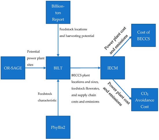
Figure 1.
Information flow diagram describing the methodology of determining the cost of implementing BECCS.
2. Materials and Methods
2.1. Power Plant Siting (OR-SAGE)
The Oak Ridge Sitting Analysis for power Generation Expansion (OR-SAGE) was used to determine potential power plant sites based on proximity to saline aquifers for CO2 storage [20]. This model, developed by Oak Ridge National Laboratory, divides the continental U.S. into 700 million cells (with an area of 2.5 acres each) and determines the proximity of each cell to critical parameters. Cells that are too far away from saline aquifers or that are within hazardous or protected areas are excluded. The OR-SAGE model considers factors such as population growth, energy demand, water availability, and geological formations and hazards when suggesting potential sites for BECCS powerplants. Figure A1 in Appendix D illustrates the gridded map of potential BECCS sites in the U.S. when exclusionary radii of 80 km and 121 km are used. This grid of the U.S. is then superimposed with potential feedstock harvesting locations provided by the Billion-Ton Report and the Biomass Logistics Information and Transport (BILT) model. A more detailed table listing the parameters considered by the OR-SAGE model can be found in Table A9 in Appendix D.
2.2. Feedstock Composition
The proximate and ultimate analyses of potential feedstock predicted by the Billion-Ton Report were determined using Phyllis2, a biomass composition database maintained by the Energy Research Center of the Netherlands (ECN) [21]. In the case of blended fuels, which account for a majority of cost estimates, a weighted average of the proximate analysis and ash composition is used. The composition of the feedstocks used in this study can be found below, in Table A1 in Appendix A. The composition of the syngas used can be found in Table A2 and Table A3 in Appendix A.
2.3. Feedstock Costs and Supply Chain
According to analysis presented in the Billion-Ton Report, the U.S. has the potential to produce approximately 1 billion tonnes of biomass capable of being used towards BECCS by the year 2040. However, not all of these resources can be used towards BECCS, since there are considerations needed regarding economic, environmental, and social factors. To account for these, biomass resources in this analysis will exclude biomass required for food, fiber, and feed. Furthermore, land allocation, risk of rain and erosion, sustainability, and conservation are considered in determining potential crops for BECCS plants. Resources that are protected or environmentally sensitive are not included, and this study ensures that demand for food, feed, fiber, and export are all met without supply disruption before being used towards BECCS. Feedstocks in this analysis include switchgrass, miscanthus, corn stover, wheat stover, pine, poplar, willow, and hardwood and softwood logging residues. The costs and emissions reported in the Billion-Ton Report for the feedstocks are inclusive of harvesting, growing, and pretreatment. Table A7 and Table A8 found in Appendix C list the costs and CO2 emissions assumed for all feedstocks used in this analysis. Information from the Billion-Ton Report is then used in the BILT model to approximate supply chain costs and emissions [22].
2.4. Power Plant Modeling
Power plant economics and performance simulations were performed using the Integrated Environmental Control Model [23]. The IECM was used to simulate the electricity generation costs and emissions of pulverized combustion and integrated combined cycle power plants running on biomass feed. PC powerplants are divided into four subsections in the IECM: Base plant, NOx control, SO2 Control, and CO2 Capture, Transport and Storage. Critical parameters used in the modeling of PC powerplants can be found in Appendix E in Table A10. IGCC powerplants are divided into seven subsections in the IECM: Overall Plant, Air Separation Unit, Gasifier Area, Sulfur Removal, CO2 Capture, Transport and Storage, and Power Block. Critical parameters used in the modeling of IGCC powerplants can be found in Appendix E in Table A11.
2.5. BECCS Scenarios
To calculate the cost of BECCS in 2040, three scenarios were developed to account for the effects of differences in feedstock preparation and power generation technologies. The three scenarios can be found in Table 1.

Table 1.
Three scenarios used to evaluate the cost of BECCS in the U.S. in 2040.
2.6. CO2 Avoidance Cost
The CO2 avoidance cost is the CO2 cost at which the energy product cost is the same for either a fossil fuel plant without CCS or the same fossil fuel plant that includes the capital and efficiency losses of adding CCS [24,25].
The CO2 Avoidance Cost (CAC) can be described by the following equation [9,26]:
where LCOE is the levelized cost of electricity, i.e., the revenue required to break even (in $ per MWh), and E is the emissions intensity of the power plant in (tonnes CO2 per MWh). BECCS refers to the power plant scenario with carbon capture and storage (BECCS), and the ref notation refers to the reference-case energy technology.
IECM calculates the ‘revenue required to break even ($ per MWh)’, which summarizes the total annual cost of running a power plant with respect to its total MWh output. A weighted LCOE was calculated using the reported revenues required to break even, number of power plants, and capacity per power plant for each BECCS scenario. Emissions intensities are also an output of the IECM program, and similar weighted averages were calculated for both BECCS and reference cases.
2.7. Cost of BECCS Equations
The cost of BECCS can be described by the following equations:
Here, the cost of electricity refers to the IECM output “revenue required to break even”. The difference between Equations (2) and (3) is that Equation (3) accounts for revenue generated by BECCS through production of electricity. Based on a 90% capacity factor, which is the fraction of operating hours per year, and the MWnet output from the IECM, annual MWh production can be calculated. The wholesale rate was determined by taking the average wholesale rate in the specified region.
2.8. Comparative Analysis Using CAC
One benefit of using CAC to describe the cost of BECCS implementation is that the equation can be used to compare two sets of power generation technologies to determine which one is most cost-effective in removing CO2 from the air. Depending on the reference-case power plant used in CAC calculations, the CAC will have a different meaning [27]. Thus, it is imperative to clearly describe the bounds for CAC in order to not misrepresent costs. Table 2 presents the different reference cases used in this study and their implications.
Table 2.
Different reference cases of power plants used in the CAC equation and their implications.
3. Results
3.1. Cost of BECCS
Figure 2 illustrates the cost of BECCS for the three BECCS scenarios considered in this study, i.e., (i) integrated biomass gasification combined cycle (IBGCC–BECCS) with non-pelletized biofuel, (ii) pulverized biomass combustion (PBC–BECCS) with pelletized biofuel, and (iii) IBGCC–BECCS with pelletized biofuel using Equations (2) and (3). In all power-generation scenarios, the cost of BECCS increases with increasing levels of CO2 sequestration and biomass utilization, because the most cost-efficient fuels (in MJ/$) are utilized initially, thus requiring the usage of the more expensive, less energy-dense feedstocks at higher levels of biomass utilization. The average fuel-intensity values (in MJ/$) for the three BECCS scenarios can be found in Figure 3, where each point represents a mixture of biomass fuels. As shown in Figure 3, the energy intensity of the 30% PBC pelletized scenario is at a maximum, and this corresponds to the minimum cost of BECCS for this scenario found in Figure 2. The cost of BECCS is the lowest in the pelletized IBGCC–BECCS scenario, and both IBGCC–BECCS scenarios (pelletized and non-pelletized) sequester CO2 at lower costs than pelletized PBC–BECCS plants. Pelletization of the feedstock before gasification in IBGCC plants decreases the cost of BECCS, due to the decrease in moisture content and the increase in the energy density of the feedstock after pelletization. Pelletization helps bring down the costs of transporting and storing the feedstock. Furthermore, pelletized feedstock can be transported longer distances without decomposing. The cost of BECCS is analogous to the LCOE, except it represents the cost per tonne of CO2 that is captured, transported, and stored by a BECCS power plant. For BECCS1 (Equation (2)), the cost of BECCS for IBGCC–BECCS pelletized plants ranges between $88 and $116 per tonne of CO2 removed from the atmosphere. BECCS2 (Equation (3)) considers the revenue generated from wholesale of electricity, and for IBGCC–BECCS pelletized plants, the cost of BECCS ranges between $62 and $83 per tonne of CO2 removed from the atmosphere.
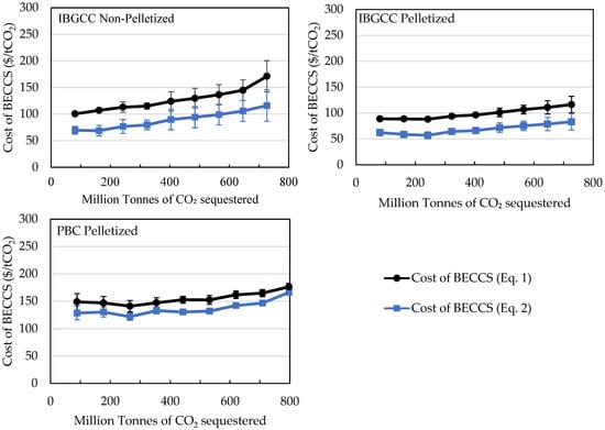
Figure 2.
Scenario-average cost of BECCS (in $ per tonne of CO2 captured) for the three BECCS scenarios. BECCS1 (Equation (2)) represents the cost of BECCS alone while BECCS2 (Equation (3)) represents the cost of BECCS with the wholesale of electricity [11].
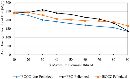
Figure 3.
Fuel intensity as a function of percent maximum biomass utilized in BECCS.
3.2. CAC Calculations Using PC Powerplants with Coal
Pulverized coal combustion (PCC) power plants were considered as a reference case for the CAC calculations, as they are the most common type of coal power plant currently found in the U.S., as well as the third-largest producer of electricity in the U.S. [28]. A PCC plant powered by bituminous Appalachian coal was used as a reference case in CAC calculations. Reference-case power plants of varying capacities were simulated in the IECM to accurately reflect the range of power plant sizes present in potential BECCS scenarios. The CAC for PBC–BECCS plants ranges between $45 and $59 per tonne of CO2 avoided when using a PCC power plant reference case without CCS. The CAC increases with increasing levels of biomass utilization due to the scarcity of inexpensive, high-energy-density feedstocks. The avoided emissions costs of other technologies reported in the literature can be found in Table 3 [29]. This cost is competitive with the CAC of neutral emissions technologies. The CAC for PBC BECCS plants ranges between $45 and $58 per tonne of CO2 avoided when using PC powerplants without CCS as the reference case. Figure 4 illustrates the range of CACs for this calculation.
Table 3.
Neutral emissions technologies and their approximate CO2 avoidance costs using a PCC power plant without CCS as reference. Data taken from Irlam et al. [29].
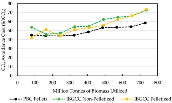
Figure 4.
CO2 avoidance costs of BECCS (in $ per tonne of CO2 avoided) using a PCC power plant without CCS as the reference case for CAC calculations.
The high CAC for solar and offshore wind can be explained by the low-capacity factors of these technologies, mainly due to their intermittent nature. Thus, it would take three to four times the capacity (in MW) to generate the same amount of MWh that a fossil fuel power plant would produce [18].
3.3. CAC Calculations Using NGCC Power Plants for Reference
Similarly to the analysis presented in the previous section, CAC calculations were conducted using an NGCC power plant as the reference case. NGCC power plants currently generate the greatest amount of electricity in the U.S. [28]. The CAC for PBC-BECCS power plants ranges between $47 and $64 per tonne of CO2 avoided when using an NGCC power plant without CCS as the reference for CAC calculations. Figure 5 illustrates the range of CACs for the three BECCS scenarios.
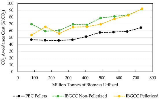
Figure 5.
CO2 avoidance costs (in $ per tonne of CO2 avoided) using an NGCC power plant without CCS as the reference case for CAC calculations.
3.4. CAC Calculations Using Biomass References
CAC calculations were also performed using power plants powered by biomass as reference plants. In this set of simulations, the PC and IGCC reference power plants were modeled to generate electricity using pelletized switchgrass feed without CCS. The CO2 avoidance cost using these reference cases helps describe the cost of carbon capture and storage in PC and IGCC technologies. The CAC for PBC–BECCS plants using PBC power plants without CCS as the reference case ranges between $39 and $61 per tonne of CO2 avoided. Figure 6 and Figure 7 illustrate the range of CACs for the three BECCS scenarios using biomass-powered reference cases. The lower CAC calculated when using IBGCC plants as the reference case reflects the higher cost of electricity generation in IBGCC systems.
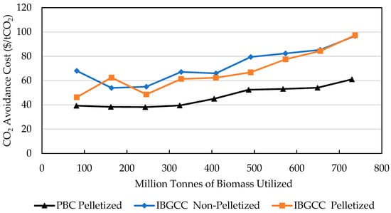
Figure 6.
CO2 avoidance cost (in $ per tonne of CO2 avoided) of BECCS using a PBC power plant reference case without CCS fueled by pelletized corn stover.
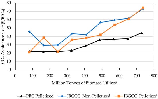
Figure 7.
CO2 avoidance cost (in $ per tonne of CO2 avoided) of BECCS using an IBGCC power plant fueled by corn stover-derived syngas as a reference case.
3.5. Corn Stover Co-Firing
Literature research indicates that a corn stover feedstock can be co-fired up to 30 weight percent in coal power plants with little technical modification [30]. The avoidance costs of co-fired power plants are explored to understand the effect of the CO2 credit experienced by a biomass co-fired feedstock. Biomass feedstock, for the purposes of CO2 accounting, can be considered to have negative emissions, because unlike coal, plants sequester atmospheric CO2 at much faster rates. Figure 8 and Figure 9 present the CAC of co-fired corn stover power plants. The CAC for a 30% corn stover co-fired plant is found to range between $70 to $104 per tonne of CO2 avoided with a PCC plant without CCS as reference. CAC values were found to decrease with increasing power plant size and co-firing percentage of biomass. Due to the benefits of economy of scale experienced by larger power plants, regardless of co-firing percent, larger power plants were found to have lower CAC. This effect of economy of scale is seen in all PC power plants simulated in this study. Increasing the percentage of co-firing decreases the CAC linearly, due to the linear decrease in the emissions intensity of co-fired power plants (based on linear increases in the CO2 credit gained by using biomass feedstocks).
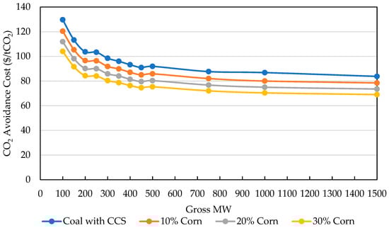
Figure 8.
Predicted CAC values for corn-stover co-fired PCC power plants with CCS. A PCC power plant without carbon capture and storage is used as the reference case for CAC calculations.
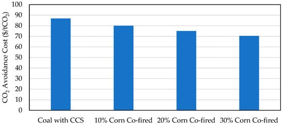
Figure 9.
CAC for a 1000-MW PCC, co-fired with corn stover power plant with CCS. A PCC power plant without carbon capture and storage is used as the reference-case plant for CAC calculations.
3.6. Poplar-Derived Bio-SNG Co-Firing
Similarly to the work presented above in the corn stover co-firing section, the cost of using BECCS feedstocks in NGCC systems was explored. Research conducted by Carbo et al. (2011) suggests that bio-SNG has the potential to sequester CO2 at low CO2 avoidance costs [31]. Literature review indicates that bio-SNG, i.e., upgraded bio-syngas, can be co-fired with fossil natural gas if the following conditions are met: a minimum CH4 percentage of 90%, and removal of sulfurous, nitrous, and chlorine-based contaminants [32]. The economics of NGCC power plants co-fired with upgraded syngas from poplar was studied, and the LCOE economics of these plants are presented in Figure 10 and Figure 11. The CAC for a 10% bio-SNG power plant using an NGCC reference case without CCS is presented in Figure 12. The LCOE for 10% co-fired NGCC plants was found to range between $119 and $127 per MWh, with larger power plants producing electricity at lower cost. The CAC for 10% co-fired NGCC plants was found to range between $145 and $162 per MWh when using an NGCC power plant without CCS as the reference case. Differences in costs can be attributed to power plant size. IBGCC–BECCS power-generating systems do not experience this economy of scale as discussed in previous sections.
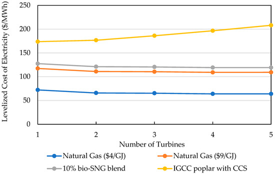
Figure 10.
Predicted LCOE for NGCC power plants co-fired with upgraded syngas produced from poplar.
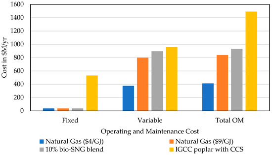
Figure 11.
Operating and Maintenance costs of co-fired 5-turbine NGCC power plants.
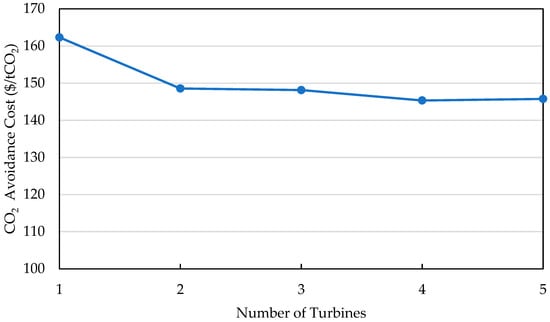
Figure 12.
CO2 avoidance cost of a 10% bio-SNG co-fired power plant with CCS. An NGCC power plant without CCS was used as the reference case for the CAC calculations. One turbine corresponds to approximately 254 net MW of power.
3.7. Comparing BECCS Power Plants to PCC Power Plants with CCS
Research conducted by Grubert et al. (2020) indicates that by the year 2035, coal power plants generating approximately 630 GW of power in the U.S. will face retirement [33]. Thus, there will be a need to construct facilities to replace the retired coal plants to meet the demand for electricity. Before moving forward and constructing facilities to generate electricity, it is important to understand the relative performances of BECCS power plants and PCC plants with CCS. In order to do this, the CAC for both BECCS power plants and PCC power plants with CCS will be calculated using a PCC power plant without CCS as the reference case. Results comparing the CAC for BECCS and PCC plants with CCS can be found in Figure 13, where it is shown that BECCS power plants operate at CO2 avoidance costs lower than those of PCC with CCS plants, with PBC plants operating at the lowest CAC cost.
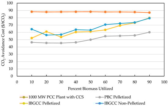
Figure 13.
CO2 avoidance cost comparison for BECCS power plants and a 1000-MW PCC power plant with CCS.
3.8. Summarized Results
A summary of the calculated ranges of CAC values for the three BECCS cases considered in this study can be found in Table 4. Results from reference cases 5 and 6 indicate that the IBGCC plants generate electricity at higher costs than PBC plants. Lastly, similar values for calculated CACs in reference cases 2 and 4 indicate that the cost of carbon capture and storage in PC and NGCC plants is similar. This similarity can be attributed to both plants based on post-combustion CO2 capture using monoethanolamine (MEA).
Table 4.
Tabulated ranges of calculated CAC for different power plant reference cases.
3.9. Future Work
To further build on our understanding of BECCS, the three following areas have been identified as potential research. The first area is with regards to quantifying the revenues gained from the wholesale of electricity. These revenues will consider the state in which the powerplant is located and the associated demand and wholesale price for electricity. The second area of potential research is with the process economics and optimization of syngas production. Understanding optimal conditions for syngas production can help reduce the cost of BECCS. Currently, there are 13 different biomass feedstocks used in our simulations, each with potentially different optimal conditions for syngas production. Should BECCS be implemented, designing a system that maximizes the heating value of the syngas produced will be crucial. The last area of research is with renewable natural gas, i.e., syngas produced from biomass capable of being used in natural gas powerplants. If syngas can be upgraded economically, the scope of BECCS can be widened to include natural gas powerplants.
4. Conclusions
BECCS has the capability of reducing the atmospheric CO2 concentration, both through sequestered atmospheric CO2 and through avoided emissions by replacing conventional coal power plants. This paper explores the potential supply of fuel and cost of BECCS under a range of feedstock options, power plant configurations and locations, and logistics. Results of the simulations performed for this paper indicated that, at a 90% capacity, BECCS in the U.S. has the potential to remove and sequester up to 737 million tonnes of CO2 per year long term from the atmosphere. According to climate goals outlined by the Paris Agreement, BECCS has the potential to sequester approximately 25% of the carbon needed to achieve carbon neutrality by 2050 in the U.S.
Scenario-specific average costs indicated that the price of capturing, transporting, and storing CO2 ranges between $88 and $116 per tonne of CO2 for pelletized IBGCC–BECCS plants, with costs increasing with increasing levels of biomass utilization. In 2020, roughly 5.4 billion metric tonnes of CO2 were released into the atmosphere in the U.S., with 1.1 billion tonnes of CO2 coming from coal power plants [4]. Converting some of these coal power plants to BECCS power plants by the year 2040 can help limit annual CO2 emissions in the U.S. to approximately 4 billion tonnes.
Calculations suggest that the CAC for pelletized PBC–BECCS plants ranges between $45 to $59 per tonne of CO2 avoided when comparing to a reference case PCC power plant without CCS. Implementation of BECCS through co-firing was also explored in the case of co-firing corn stover with coal and bio-SNG with fossil natural gas. For 30% corn stover co-firing, the CAC ranges between $70 and $104 per tonne of CO2 avoided. The CAC for 1000-MW co-fired stover PCC plants with CCS ranges between $70 to $87 per MWh, with the CAC decreasing with increasing biomass co-firing percentages. In bio-SNG co-fired NGCC plants, the LCOE was seen to range between $119 and $127 per MWh, depending on the size of the plant. The CAC for a 10% co-fired bio-SNG plant ranges between $145 and $162 per MWh when using an NGCC plant without CCS as the reference case. For PBC reference-case plants without CCS, the CAC for BECCS was seen to range between $39 and $61 per tonne of CO2 avoided for BECCS–PBC plants, and between $46 and $97 per tonne of CO2 avoided for IBGCC–BECCS plants.
Results from this study indicate that PBC plants will be the most cost-effective power-generation technology to implement BECCS in the U.S. A comparative analysis of the CAC of BECCS and other energy technologies suggests that BECCS can generate electricity competitively with neutral emissions technologies while having a net-negative CO2 footprint. Furthermore, comparative results presented in this study indicate that BECCS can operate with CAC values below those of PCC plants with CCS. Results presented in this study indicate that the CAC of BECCS is lower than that of solar and offshore wind, but higher than onshore wind and nuclear. Finally, it should be noted that several assumptions are involved in the model development and predictions. Better understanding of biomass pretreatment, gasification and conversion to power through research and development would greatly improve predictions and reduce the risks.
Author Contributions
Conceptualization, A.K.; methodology, A.K., M.L., I.B., C.T.; software, A.K., I.B., M.H.; validation, I.B., M.H., J.M.; formal analysis, A.K., C.T., M.L.; investigation, A.K., I.B., M.L., C.T.; resources, S.Y., C.T., M.L.; data curation, A.K., I.B.; writing—original draft preparation, A.K., S.Y., C.T., M.L.; writing—review and editing, A.K., C.T., M.L., S.Y., I.B., M.H., J.M.; visualization, A.K., M.L., I.B.; supervision, C.T., S.Y., M.L.; project administration, C.T., M.L., S.Y.; funding acquisition, M.L. All authors have read and agreed to the published version of the manuscript.
Funding
This research was supported by the US Department of Energy (DOE), Office of Energy Efficiency and Renewable Energy (EERE), Bioenergy Technologies Office (BETO), and by the DOE Office of Fossil Energy and Carbon Management under Contract Number DE-AC05-00OR22725.
Institutional Review Board Statement
Not applicable.
Informed Consent Statement
Not applicable.
Data Availability Statement
Not applicable.
Conflicts of Interest
The authors declare no conflict of interest.
Appendix A. Fuel and Syngas Compositions
Table A1.
Syngas composition used in IBGCC simulations.
Table A1.
Syngas composition used in IBGCC simulations.
| C2H4 | C2H6 | C3H6 | C3H8 | CH4 | CO | CO2 | H2 | O2 | |
|---|---|---|---|---|---|---|---|---|---|
| Barley Straw | 0.0 | 0.0 | 0.0 | 0.0 | 0.7 | 51.8 | 1.0 | 43.9 | 0.0 |
| Corn Stover | 4.2 | 0.0 | 0.1 | 0.4 | 15.3 | 27.2 | 23.7 | 26.9 | 0.0 |
| Hardwood | 0.0 | 0.0 | 0.0 | 0.0 | 3.1 | 46.9 | 28.3 | 21.7 | 1.7 |
| Miscanthus | 0.0 | 0.0 | 0.0 | 0.0 | 9.3 | 25.6 | 23.4 | 41.7 | 0.0 |
| Mixedwood | 1.2 | 0.0 | 0.0 | 0.0 | 8.5 | 27.8 | 17.0 | 45.6 | 0.8 |
| Oats straw | 0.7 | 2.9 | 1.0 | 0.0 | 20.3 | 33.9 | 20.4 | 20.7 | 0.0 |
| Pine | 0.0 | 0.0 | 0.0 | 0.0 | 11.4 | 35.3 | 33.8 | 19.5 | 0.0 |
| Poplar | 1.9 | 0.1 | 0.0 | 0.0 | 8.6 | 23.2 | 20.8 | 45.4 | 0.0 |
| Softwood | 2.3 | 0.0 | 0.0 | 0.0 | 14.0 | 8.6 | 5.6 | 69.5 | 0.0 |
| Sorghum | 0.0 | 1.0 | 0.0 | 0.0 | 9.8 | 41.8 | 33.5 | 12.5 | 0.0 |
| Switchgrass | 0.0 | 0.0 | 0.0 | 0.0 | 9.3 | 25.6 | 23.4 | 41.7 | 0.0 |
| Wheat straw | 4.3 | 0.0 | 0.1 | 0.8 | 16.3 | 29.0 | 22.0 | 25.4 | 0.0 |
| Willow | 0.1 | 0.2 | 0.0 | 0.1 | 3.4 | 62.5 | 8.6 | 18.9 | 6.1 |
Table A2.
Proximate analysis of non-pelletized biomass feedstocks used for PBC and IBGCC simulations.
Table A2.
Proximate analysis of non-pelletized biomass feedstocks used for PBC and IBGCC simulations.
| Component | H2O (%) | Ash (%) | C (%) | H (%) | N (%) | S (%) | O (%) | Cl (%) | LHV (kJ/kg) | HHV (kJ/kg) |
|---|---|---|---|---|---|---|---|---|---|---|
| Barley Straw | 10.0 | 4.5 | 41.9 | 5.0 | 0.5 | 0.1 | 37.5 | 0.5 | 15,300.0 | 16,646.7 |
| Corn stover | 20.0 | 4.8 | 36.5 | 4.6 | 0.5 | 0.1 | 33.2 | 0.0 | 13,113.3 | 14,424.7 |
| Hardwood | 50.0 | 1.1 | 26.2 | 3.1 | 0.1 | 0.0 | 19.9 | 0.0 | 8946.7 | 10,816.7 |
| Mixedwood | 50.0 | 1.4 | 26.2 | 3.0 | 0.2 | 0.0 | 19.3 | 0.0 | 8790.0 | 10,658.3 |
| Oats Straw | 10.0 | 6.2 | 42.3 | 4.8 | 0.5 | 0.1 | 37.0 | 0.7 | 15,365.0 | 16,665.0 |
| Pine | 40.0 | 2.4 | 31.2 | 3.4 | 0.2 | 0.0 | 22.8 | 0.0 | 10,672.0 | 12,272.8 |
| Poplar | 40.0 | 1.1 | 29.3 | 3.6 | 0.2 | 0.0 | 25.9 | 0.0 | 10,036.0 | 11,541.4 |
| Softwood | 50.0 | 1.7 | 26.2 | 3.0 | 0.3 | 0.1 | 18.7 | 0.0 | 8633.3 | 10,500.0 |
| Sorghum | 20.0 | 5.6 | 36.7 | 4.0 | 0.6 | 0.0 | 32.8 | 0.2 | 13,103.3 | 14,466.7 |
| Switchgrass | 15.0 | 6.1 | 40.2 | 4.9 | 0.6 | 0.1 | 32.9 | 0.0 | 14,160.0 | 16,284.0 |
| Miscanthus | 15.0 | 6.1 | 40.2 | 4.9 | 0.6 | 0.1 | 32.9 | 0.0 | 14,160.0 | 16,284.0 |
| Wheat Straw | 10.0 | 5.0 | 41.4 | 5.1 | 1.0 | 0.1 | 36.8 | 0.3 | 15,866.7 | 17,293.3 |
| Willow | 50.0 | 0.8 | 24.8 | 3.1 | 0.3 | 0.0 | 21.1 | 0.0 | 9683.3 | 9950.0 |
Table A3.
Proximate analysis of pelletized biomass feedstocks used for PBC and IBGCC simulations.
Table A3.
Proximate analysis of pelletized biomass feedstocks used for PBC and IBGCC simulations.
| Component | H2O (%) | Ash (%) | C (%) | H (%) | N (%) | S (%) | O (%) | Cl (%) | LHV (kJ/kg) | HHV (kJ/kg) |
|---|---|---|---|---|---|---|---|---|---|---|
| Barley Straw | 10.0 | 4.5 | 41.9 | 5.0 | 0.5 | 0.1 | 37.5 | 0.0 | 15,300.0 | 16,830.0 |
| Corn Stover | 10.0 | 5.4 | 41.1 | 5.1 | 0.5 | 0.1 | 37.3 | 0.0 | 15,060.0 | 16,566.0 |
| Hardwood | 10.0 | 1.4 | 47.1 | 5.6 | 0.2 | 0.0 | 35.8 | 0.0 | 18,060.0 | 19,866.0 |
| Miscanthus | 9.0 | 6.6 | 43.0 | 5.3 | 0.6 | 0.1 | 35.3 | 0.0 | 15,330.0 | 16,863.0 |
| Mixedwood | 10.0 | 2.2 | 47.1 | 5.4 | 0.4 | 0.1 | 34.8 | 0.0 | 17,776.7 | 19,554.3 |
| Oats Straw | 10.0 | 6.2 | 42.3 | 4.8 | 0.5 | 0.1 | 37.0 | 0.0 | 15,365.0 | 16,901.5 |
| Pine | 10.0 | 3.6 | 46.8 | 5.1 | 0.3 | 0.0 | 34.2 | 0.0 | 17,100.0 | 18,810.0 |
| Poplar | 10.0 | 1.6 | 43.9 | 5.4 | 0.2 | 0.0 | 38.8 | 0.0 | 16,274.0 | 17,901.4 |
| Softwood | 10.0 | 3.1 | 47.2 | 5.3 | 0.6 | 0.2 | 33.7 | 0.0 | 17,493.3 | 19,242.7 |
| Sorghum | 10.0 | 6.3 | 41.3 | 4.5 | 0.7 | 0.0 | 36.9 | 0.0 | 15,043.3 | 16,547.7 |
| Switchgrass | 9.0 | 6.6 | 43.0 | 5.3 | 0.6 | 0.1 | 35.3 | 0.0 | 15,330.0 | 16,863.0 |
| Wheat Straw | 10.0 | 5.0 | 41.4 | 5.1 | 1.0 | 0.1 | 36.8 | 0.0 | 15,866.7 | 17,453.3 |
| Willow | 10.0 | 1.4 | 44.6 | 5.5 | 0.5 | 0.0 | 38.0 | 0.0 | 15,973.3 | 17,570.7 |
Appendix B. CO2 Avoidance Cost Information
Table A4.
Levelized Cost of Electricity (LCOE, in $/MWh) and Emissions Intensity (E, in tCO2/MWh) for the four CAC reference cases and PBC powerplants.
Table A4.
Levelized Cost of Electricity (LCOE, in $/MWh) and Emissions Intensity (E, in tCO2/MWh) for the four CAC reference cases and PBC powerplants.
| PBC Pellets | PC Coal no CCS (Ref) | NGCC no CCS (Ref) | PC Biomass no CCS (Ref) | IGCC Biomass no CCS (Ref) | ||||||||||
|---|---|---|---|---|---|---|---|---|---|---|---|---|---|---|
| tCO2 | LCOECCS | ECCS | LCOEref | Eref | ESupply Chain | LCOEref | Eref | ESupply Chain | LCOEref | Eref | ESupply Chain | LCOEref | Eref | ESupply Chain |
| 81 | 144.49 | −1.37 | 43.00 | 0.82 | 0.06 | 61.96 | 0.36 | 0.02 | 88.36 | 0 | 0.06 | 112.8 | 0 | 0.06 |
| 162 | 144.71 | −1.41 | 43.23 | 0.82 | 0.06 | 61.96 | 0.36 | 0.02 | 88.36 | 0 | 0.06 | 112.8 | 0 | 0.06 |
| 243 | 145.04 | −1.42 | 43.12 | 0.82 | 0.06 | 61.96 | 0.36 | 0.02 | 88.36 | 0 | 0.06 | 112.8 | 0 | 0.06 |
| 324 | 147.24 | −1.43 | 43.05 | 0.82 | 0.06 | 61.96 | 0.36 | 0.02 | 88.36 | 0 | 0.06 | 112.8 | 0 | 0.06 |
| 405 | 155.10 | −1.42 | 43.00 | 0.82 | 0.06 | 61.96 | 0.36 | 0.02 | 88.36 | 0 | 0.06 | 112.8 | 0 | 0.06 |
| 487 | 165.75 | −1.41 | 43.18 | 0.82 | 0.06 | 61.96 | 0.36 | 0.02 | 88.36 | 0 | 0.06 | 112.8 | 0 | 0.06 |
| 568 | 166.89 | −1.42 | 43.17 | 0.82 | 0.06 | 61.96 | 0.36 | 0.02 | 88.36 | 0 | 0.06 | 112.8 | 0 | 0.06 |
| 649 | 167.50 | −1.40 | 43.33 | 0.82 | 0.06 | 61.96 | 0.36 | 0.02 | 88.36 | 0 | 0.06 | 112.8 | 0 | 0.06 |
| 730 | 177.30 | −1.40 | 43.80 | 0.82 | 0.06 | 61.96 | 0.36 | 0.02 | 88.36 | 0 | 0.06 | 112.8 | 0 | 0.06 |
| 803 | 194.56 | −1.35 | 43.00 | 0.82 | 0.06 | 61.96 | 0.36 | 0.02 | 88.36 | 0 | 0.06 | 112.8 | 0 | 0.06 |
| 811 | 195.29 | −1.34 | 43.03 | 0.82 | 0.06 | 61.96 | 0.36 | 0.02 | 88.36 | 0 | 0.06 | 112.8 | 0 | 0.06 |
Table A5.
Levelized Cost of Electricity (LCOE, in $/MWh) and Emissions Intensity (E, in tCO2/MWh) for the four CAC reference cases and IBGCC non-pelletized powerplants.
Table A5.
Levelized Cost of Electricity (LCOE, in $/MWh) and Emissions Intensity (E, in tCO2/MWh) for the four CAC reference cases and IBGCC non-pelletized powerplants.
| IBGCC Non-Pellets | PC Coal no CCS (Ref) | NGCC no CCS (Ref) | PC Biomass no CCS (Ref) | IGCC Biomass no CCS (Ref) | ||||||||||
|---|---|---|---|---|---|---|---|---|---|---|---|---|---|---|
| tCO2 | LCOECCS | ECCS | LCOEref | Eref | ESupply Chain | LCOEref | Eref | ESupply Chain | LCOEref | Eref | ESupply Chain | LCOEref | Eref | ESupply Chain |
| 82 | 157.57 | −0.96 | 58.40 | 0.83 | 0.06 | 63.76 | 0.36 | 0.02 | 88.36 | 0 | 0.06 | 112.8 | 0 | 0.02 |
| 164 | 139.39 | −0.88 | 57.95 | 0.83 | 0.06 | 63.71 | 0.36 | 0.02 | 88.36 | 0 | 0.06 | 112.8 | 0 | 0.02 |
| 246 | 139.19 | −0.86 | 56.07 | 0.83 | 0.06 | 63.51 | 0.36 | 0.02 | 88.36 | 0 | 0.06 | 112.8 | 0 | 0.02 |
| 328 | 152.78 | −0.90 | 55.69 | 0.83 | 0.06 | 63.47 | 0.36 | 0.02 | 88.36 | 0 | 0.06 | 112.8 | 0 | 0.02 |
| 410 | 151.35 | −0.89 | 53.32 | 0.83 | 0.06 | 63.21 | 0.36 | 0.02 | 88.36 | 0 | 0.06 | 112.8 | 0 | 0.02 |
| 491 | 166.83 | −0.93 | 53.55 | 0.83 | 0.06 | 63.24 | 0.36 | 0.02 | 88.36 | 0 | 0.06 | 112.8 | 0 | 0.02 |
| 573 | 168.10 | −0.91 | 51.91 | 0.82 | 0.06 | 63.05 | 0.36 | 0.02 | 88.36 | 0 | 0.06 | 112.8 | 0 | 0.02 |
| 655 | 168.60 | −0.88 | 51.16 | 0.82 | 0.06 | 62.97 | 0.36 | 0.02 | 88.36 | 0 | 0.06 | 112.8 | 0 | 0.02 |
| 737 | 177.73 | −0.86 | 50.41 | 0.82 | 0.06 | 62.88 | 0.36 | 0.02 | 88.36 | 0 | 0.06 | 112.8 | 0 | 0.02 |
| 82 | 157.57 | −0.96 | 58.40 | 0.83 | 0.06 | 63.76 | 0.36 | 0.02 | 88.36 | 0 | 0.06 | 112.8 | 0 | 0.02 |
| 164 | 139.39 | −0.88 | 57.95 | 0.83 | 0.06 | 63.71 | 0.36 | 0.02 | 88.36 | 0 | 0.06 | 112.8 | 0 | 0.02 |
Table A6.
Levelized Cost of Electricity (LCOE, in $/MWh) and Emissions Intensity (E, in tCO2/MWh) for the four CAC reference cases and IBGCC non-pelletized powerplants.
Table A6.
Levelized Cost of Electricity (LCOE, in $/MWh) and Emissions Intensity (E, in tCO2/MWh) for the four CAC reference cases and IBGCC non-pelletized powerplants.
| IBGCC Pellets | PC Coal no CCS (Ref) | NGCC no CCS (Ref) | PC Biomass no CCS (Ref) | IGCC Biomass no CCS (Ref) | ||||||||||
|---|---|---|---|---|---|---|---|---|---|---|---|---|---|---|
| tCO2 | LCOECCS | ECCS | LCOEref | Eref | ESupply Chain | LCOEref | Eref | ESupply Chain | LCOEref | Eref | ESupply Chain | LCOEref | Eref | ESupply Chain |
| 82 | 131.80 | −0.88 | 57.53 | 0.83 | 0.06 | 63.67 | 0.36 | 0.02 | 88.36 | 0 | 0.06 | 112.8 | 0 | 0.02 |
| 164 | 148.42 | −0.90 | 56.65 | 0.83 | 0.06 | 63.57 | 0.36 | 0.02 | 88.36 | 0 | 0.06 | 112.8 | 0 | 0.02 |
| 246 | 131.26 | −0.82 | 55.81 | 0.83 | 0.06 | 63.48 | 0.36 | 0.02 | 88.36 | 0 | 0.06 | 112.8 | 0 | 0.02 |
| 328 | 144.16 | −0.85 | 55.17 | 0.83 | 0.06 | 63.42 | 0.36 | 0.02 | 88.36 | 0 | 0.06 | 112.8 | 0 | 0.02 |
| 410 | 147.72 | −0.89 | 53.04 | 0.83 | 0.06 | 63.18 | 0.36 | 0.02 | 88.36 | 0 | 0.06 | 112.8 | 0 | 0.02 |
| 491 | 149.73 | −0.86 | 52.07 | 0.82 | 0.06 | 63.07 | 0.36 | 0.02 | 88.36 | 0 | 0.06 | 112.8 | 0 | 0.02 |
| 573 | 161.96 | −0.89 | 51.45 | 0.82 | 0.06 | 63.00 | 0.36 | 0.02 | 88.36 | 0 | 0.06 | 112.8 | 0 | 0.02 |
| 649 | 167.50 | −1.40 | 43.33 | 0.82 | 0.06 | 61.96 | 0.36 | 0.02 | 88.36 | 0 | 0.06 | 112.8 | 0 | 0.06 |
| 730 | 177.30 | −1.40 | 43.80 | 0.82 | 0.06 | 61.96 | 0.36 | 0.02 | 88.36 | 0 | 0.06 | 112.8 | 0 | 0.06 |
| 803 | 194.56 | −1.35 | 43.00 | 0.82 | 0.06 | 61.96 | 0.36 | 0.02 | 88.36 | 0 | 0.06 | 112.8 | 0 | 0.06 |
| 811 | 195.29 | −1.34 | 43.03 | 0.82 | 0.06 | 61.96 | 0.36 | 0.02 | 88.36 | 0 | 0.06 | 112.8 | 0 | 0.06 |
Appendix C. Biomass Resources Information
Table A7.
Costs (inclusive of harvesting and handling) for fuels used in this study. These results serve as an input for the BILT model [11].
Table A7.
Costs (inclusive of harvesting and handling) for fuels used in this study. These results serve as an input for the BILT model [11].
| Resource Category | Resource | $44 | $66 | $88 | $110 |
|---|---|---|---|---|---|
| Crop residues | Barley straw | 3.82 × 10⁵ | 5.16 × 10⁵ | 5.67 × 10⁵ | 5.88 × 10⁵ |
| Corn stover | 4.03 × 10⁷ | 1.40 × 10⁸ | 1.51 × 10⁸ | 1.50 × 10⁸ | |
| Oats straw | 6.02 × 10³ | 7.39 × 10³ | 6.90 × 10³ | 6.85 × 10³ | |
| Wheat straw | 1.11 × 10⁷ | 1.89 × 10⁷ | 1.79 × 10⁷ | 1.80 × 10⁷ | |
| Sorghum stubble | 7.72 × 10⁵ | 9.56 × 10⁵ | 1.05 × 10⁶ | 9.80 × 10⁵ | |
| Herbaceous energy | Energy cane | 0 | 3.03 × 10⁵ | 1.52 × 10⁶ | 4.03 × 10⁶ |
| crops | Miscanthus | 5.90 × 10⁶ | 1.45 × 10⁸ | 2.66 × 10⁸ | 2.98 × 10⁸ |
| Biomass sorghum | 8.11 × 10⁵ | 1.75 × 10⁷ | 5.28 × 10⁷ | 8.67 × 10⁷ | |
| Switchgrass | 2.45 × 10⁷ | 1.46 × 10⁸ | 1.25 × 10⁸ | 1.10 × 10⁸ | |
| Logging residues | Hardwood, lowland logging residues | 4.21 × 10⁶ | 4.21 × 10⁶ | 4.21 × 10⁶ | 4.21 × 10⁶ |
| Hardwood, upland logging residues | 3.09 × 10⁶ | 3.09 × 10⁶ | 3.09 × 10⁶ | 3.09 × 10⁶ | |
| Mixedwood logging residues | 2.45 × 10⁶ | 2.45 × 10⁶ | 2.45 × 10⁶ | 2.45 × 10⁶ | |
| Softwood, natural logging residues | 7.43 × 10⁶ | 7.43 × 10⁶ | 7.43 × 10⁶ | 7.43 × 10⁶ | |
| Softwood, planted logging residues | 1.68 × 10⁶ | 1.68 × 10⁶ | 1.68 × 10⁶ | 1.68 × 10⁶ | |
| Hardwood, lowland whole trees | 0 | 8.31 × 10⁶ | 2.20 × 10⁷ | 2.20 × 10⁷ | |
| Hardwood, upland whole trees | 0 | 1.42 × 10⁷ | 2.73 × 10⁷ | 2.73 × 10⁷ | |
| Whole trees | Mixedwood whole trees | 3.45 × 10⁴ | 2.16 × 10⁶ | 2.33 × 10⁶ | 2.33 × 10⁶ |
| Softwood, natural whole trees | 0 | 1.55 × 10⁷ | 1.98 × 10⁷ | 1.98 × 10⁷ | |
| Softwood, planted whole trees | 0 | 1.49 × 10⁷ | 1.49 × 10⁷ | 1.49 × 10⁷ | |
| Eucalyptus | 0 | 8.50 × 10⁵ | 5.67 × 10⁵ | 4.70 × 10⁵ | |
| Woody energy | Pine | 0 | 1.08 × 10⁵ | 1.55 × 10⁴ | 3.47 × 10³ |
| crops | Poplar | 7.69 × 10⁶ | 4.07 × 10⁷ | 3.75 × 10⁷ | 4.22 × 10⁷ |
| Willow | 6.55 × 10⁶ | 2.28 × 10⁷ | 1.28 × 10⁷ | 6.95 × 10⁶ |
Table A8.
Carbon emissions associated with production, harvesting, and transportation of the different feedstocks used in this study. These results serve as an input for the BILT model [11].
Table A8.
Carbon emissions associated with production, harvesting, and transportation of the different feedstocks used in this study. These results serve as an input for the BILT model [11].
| Feedstock | Production and Harvest | Power Generation | Transportation | Form |
|---|---|---|---|---|
| Barley straw | 73 | 133.9 | 0.1587 | Pellet |
| 0.1785 | Raw | |||
| Biomass sorghum | 107.7 | 133.9 | 0.1587 | Pellet |
| 0.1785 | Raw | |||
| Corn stover | 54.3 | 133.9 | 0.1587 | Pellet |
| 0.1785 | Raw | |||
| Hardwood, lowland logging | 5.2 | 107.4 | 0.1586 | Pellet |
| residues | 0.238 | Raw | ||
| Hardwood, lowland whole | 14.4 | 107.4 | 0.1586 | Pellet |
| trees | 0.238 | Raw | ||
| Hardwood, upland logging | 5.3 | 107.4 | 0.1586 | Pellet |
| residues | 0.238 | Raw | ||
| Hardwood, upland whole | 14.7 | 107.4 | 0.1586 | Pellet |
| trees | 0.238 | Raw | ||
| Miscanthus | 84.9 | 147.4 | 0.1569 | Pellet |
| 0.168 | Raw | |||
| Mixedwood logging residues | 5.2 | 107.4 | 0.1586 | Pellet |
| 0.238 | Raw | |||
| Mixedwood whole trees | 15.2 | 107.4 | 0.1586 | Pellet |
| 0.238 | Raw | |||
| Pine | 123.5 | 191 | 0.1586 | pellet |
| 0.238 | raw | |||
| Poplar | 64.1 | 107.4 | 0.1586 | pellet |
| 0.238 | raw | |||
| Softwood, natural logging | 5.2 | 107.4 | 0.1586 | pellet |
| residues | 0.238 | raw | ||
| Softwood, natural whole | 14.7 | 107.4 | 0.1586 | pellet |
| trees | 0.238 | raw | ||
| Softwood, planted logging | 5.4 | 107.4 | 0.1586 | pellet |
| residues | 0.238 | raw | ||
| Softwood, planted whole | 16.6 | 107.4 | 0.1586 | pellet |
| trees | 0.238 | raw | ||
| Sorghum stubble | 60.5 | 133.9 | 0.1587 | pellet |
| 0.1785 | raw | |||
| Switchgrass | 61.3 | 147.4 | 0.1569 | pellet |
| 0.168 | raw | |||
| Wheat straw | 47.8 | 133.9 | 0.1587 | pellet |
| 0.1785 | raw | |||
| Willow | 129.5 | 107.4 | 0.1586 | pellet |
| 0.238 | raw |
Appendix D. OR-SAGE Model
Table A9.
Exclusionary parameters and their values used in OR-SAGE to determine potential sites for BECCS powerplants [11].
Table A9.
Exclusionary parameters and their values used in OR-SAGE to determine potential sites for BECCS powerplants [11].
| Criteria | Exclusion Value |
|---|---|
| Population Density | >195 per km2 |
| Wetlands | No |
| Open Water | No |
| Protected lands | No |
| Slope | >12% |
| Landslide Hazards (moderate or high) | No |
| 100-year floodplain | No |
| Cooling water within 32km | 473,000 L per min |
| Geological formations | Outside saline basin |
| Non-Attainment Areas (EPA) | No |

Figure A1.
(A) Potential sites thinned to a distance of 80 km (171 sites). (B) Potential sites thinned to a distance of 121 km (103 sites) [11].
Figure A1.
(A) Potential sites thinned to a distance of 80 km (171 sites). (B) Potential sites thinned to a distance of 121 km (103 sites) [11].

Appendix E. IECM Model Parameters
Table A10.
Modeling parameters used for pulverized combustion (PC) powerplants in the IECM.
Table A10.
Modeling parameters used for pulverized combustion (PC) powerplants in the IECM.
| Plant Section | Parameter | Value |
|---|---|---|
| Base Plant | Gross MW | 100 MW to 1500 MW |
| Unit Type | Supercritical | |
| Steam Cycle Heat Rate | 1.047 × 10⁴ kJ/kWh | |
| Boiler Firing Type | Tangential | |
| Boiler Efficiency | 87.5% | |
| Excess Air for Furnace | 20% | |
| Leakage Air at Preheater | 10% | |
| NOx Control | In-Furnace Controls | LNB |
| LNB Actual NOx Removal Efficiency (%) | 44.39% | |
| Hot Side SCR NOx Removal Efficiency | 50% | |
| SO2 Control | Reagent | Limestone |
| Scrubber SO2 Removal Efficiency | 98% | |
| Scrubber SO3 Removal Efficiency | 50% | |
| Particulate Removal Efficiency | 50% | |
| Reagent Stoichiometry | 1.03 mol Ca/mol S | |
| Reagent Purity | 92.4% | |
| CO2 Capture, Transport and Storage | System Used | MEA |
| Compressor Type | 6-stage | |
| CO2 Removal Efficiency | 90% | |
| Sorbent Concentration | 30% | |
| Lean CO2 Loading | 0.2 mol CO2/mol MEA | |
| Sorbent Losses | 2.25 kg/tCO2 | |
| Sorbent Recovered | 0.1985 kg/tCO2 | |
| Liquid to Gas Ratio | 3.29 | |
| Regeneration Heat Requirement | 4529 kJ/kg CO2 | |
| Regeneration Steam Heat Content | 3194 kJ/kg steam | |
| Heat-to-Electricity Efficiency | 18.7% | |
| CO2 Product Pressure | 13.79 MPa | |
| CO2 Compressor Efficiency | 80% | |
| CO2 Unit Compression Energy | 117.9 kWh/tCO2 | |
| CO2 Transport Method | Pipeline | |
| CO2 Storage Method | Geologic | |
| Pipeline Length | 100 m | |
| Booster Pump Efficiency | 75% | |
| Min Outlet Pressure | 10.39 | |
| Reservoir Depth | 1219 m | |
| Reservoir Thickness | 304 m | |
| Reservoir Horizontal Permeability | 100 mD | |
| Reservoir Porosity | 12% | |
| Performance Model | Law and Bachu |
Table A11.
Modeling parameters used for integrated gasification combined cycle (IGCC) powerplants in the IECM.
Table A11.
Modeling parameters used for integrated gasification combined cycle (IGCC) powerplants in the IECM.
| Plant Section | Parameter | Value |
|---|---|---|
| Overall Plant | Number of Turbines | 1 to 5 |
| Capacity Factor | 90% | |
| Ambient Air Temperature | 18.89 °C | |
| Air Separation Unit | Oxidation O2% | 95% |
| Oxidation Ar% Efficiency | 4.24% | |
| Oxidation N2% | 0.76% | |
| Unit Separation Energy | 6860 kWh/tonne | |
| Gasifier Area | Gasifier Temperature | 1343 °C |
| Gasifier Pressure | 44.24 MPa | |
| Total Water Input | 1.274 mol H2O/mol C | |
| Carbon in Slag | 3% | |
| Sulfur Removal | COS to H2S Conversion Efficiency | 98.5% |
| H2S removal Efficiency | 98% | |
| COS Removal Efficiency | 33% | |
| CO2 Removal Efficiency | 0% | |
| Claus Plant S Removal Efficiency | 95% | |
| Claus Plant S capacity | 4.5 tonne/hr | |
| Claus Plant Power Required | 0.7% MWgross | |
| Tailgas S Recovered | 99% | |
| Tailgas Power Required | 0.2% MWgross | |
| CO2 Capture, Transport and Storage | WGSR CO to CO2 Conversion | 95% |
| WGSR COS to H2S Conversion | 98.5% | |
| WGSR Steam Added | 0.99 mol H2O/mol CO | |
| WGSR Capacity | 140 tonne CO2/h | |
| WGSR Thermal Energy Credit | 117.9 kWh/tCO2 | |
| Selexol CO2 Removal Efficiency | 95% | |
| Selexol H2S Removal Efficiency | 94% | |
| Syngas Capacity | 287 tonne CO2/h | |
| CO2 Product Pressure | 13.79 MPa | |
| CO2 Compressor Efficiency | 80% | |
| CO2 Unit Compression Energy | 117.9 kWh/tCO2 | |
| CO2 Transport Method | Pipeline | |
| CO2 Storage Method | Geologic | |
| Pipeline Length | 100 m | |
| Booster Pump Efficiency | 75% | |
| Min Outlet Pressure | 10.39 | |
| Reservoir Depth | 1219 m | |
| Reservoir Thickness | 304 m | |
| Reservoir Horizontal Permeability | 100 mD | |
| Reservoir Porosity | 12% | |
| Performance Model | Law and Bachu | |
| Power Block | Gas Turbine Model | GE 7FB |
| Number of Gas Turbines | 1–5 | |
| Flue Gas Moisture Content | 33% | |
| Turbine Inlet Temperature | 1371 °C | |
| Air Compressor Pressure Ratio | 18.5 (outlet:inlet) | |
| Air Compressor Adiabatic Compressor Efficiency | 87.5% | |
| Combustor Inlet Pressure | 1.875 MPa |
References
- Aaron, D.; Tsouris, C. Separation of CO2 from flue gas: A review. Sep. Sci. Technol. 2005, 40, 321–348. [Google Scholar] [CrossRef]
- Bolton, S.; Kasturi, A.; Palko, S.; Lai, C.; Love, L.; Parks, J.; Xin, S.; Tsouris, C. 3D printed structures for optimized carbon capture technology in packed bed columns. Sep. Sci. Technol. 2019, 54, 2047–2058. [Google Scholar] [CrossRef]
- EPA. Sources of Greenhouse Gas Emissions. Agency. 2019. Available online: https://www.epa.gov/ghgemissions/sources-greenhouse-gas-emissions (accessed on 1 March 2021).
- U.S. Energy Information Administration (EIA). U.S. Energy-Related Carbon Dioxide Emissions; U.S. Energy Information Administration (EIA): Washington, DC, USA, 2019.
- EPA. Inventory of US Greenhouse Emissions and Sinks. Agency. 2019. Available online: https://www.epa.gov/ghgemissions/inventory-us-greenhouse-gas-emissions-and-sinks-1990-2019 (accessed on 1 March 2021).
- DOE. Iron and Steel Sector (NAICS 3311 and 3312) Energy and GHG Combustion Emissions Profile; US Department of Energy: Washington, DC, USA, 2012.
- IPCC. Special Report on Global Warming of 1.5 °C; Intergovernmental Panel on Climate Change: Geneva, Switzerland, 2019. [Google Scholar]
- Fajardy, M.; Mac Dowell, N. Can BECCS deliver sustainable and resource efficient negative emissions? Energy Environ. Sci. 2017, 10, 1389–1426. [Google Scholar] [CrossRef]
- Emenike, O.; Michailos, S.; Finney, K.N.; Hughes, K.J.; Ingham, D.; Pourkashanian, M. Initial techno-economic screening of BECCS technologies in power generation for a range of biomass feedstock. Sustain. Energy Technol. Assess. 2020, 40, 100743. [Google Scholar] [CrossRef]
- Strauss, W. Industrial wood pellet fuel in pulverized coal power plants a rational, pragmatic, and easy to implement solution for transitioning toward a zero coal future in Alberta. In Proceedings of the Compliance Strategies and New Development Opportunities, Calgary, AB, Canada, 26–27 September 2016. [Google Scholar]
- Langholtz, M.; Busch, I.; Kasturi, A.; Hilliard, M.; McFarlane, J.; Tsouris, C.; Mukherjee, S.; Omitaomu, O.; Kotikot, S.; Allen-Dumas, M.; et al. The economic accessibility of CO2 sequestration through bioenergy with carbon capture and storage (BECCS) in the US. Land 2020, 9, 299. [Google Scholar] [CrossRef]
- Baik, E.; Sanchez, D.L.; Turner, P.A.; Mach, K.J.; Field, C.B.; Benson, S.M. Geospatial analysis of near-term potential for carbon-negative bioenergy in the United States. Proc. Natl. Acad. Sci. USA 2018, 115, 3290–3295. [Google Scholar] [CrossRef] [PubMed]
- Köberle, A.C. The value of BECCS in IAMs: A review. Curr. Sustain. Energy Rep. 2019, 6, 107–115. [Google Scholar] [CrossRef]
- Shahbaz, M.; AlNouss, A.; Ghiat, I.; Mckay, G.; Mackey, H.; Elkhalifa, S.; Al-Ansari, T. A comprehensive review of biomass based thermochemical conversion technologies integrated with CO2 capture and utilisation within BECCS networks. Resour. Conserv. Recycl. 2021, 173, 105734. [Google Scholar] [CrossRef]
- Inayat, M.; Sulaiman, S.A.; Shahbaz, M.; Bhayo, B.A. Application of response surface methodology in catalytic co-gasification of palm wastes for bioenergy conversion using mineral catalysts. Biomass-Bioenergy 2020, 132, 105418. [Google Scholar] [CrossRef]
- Chan, Y.H.; Cheah, K.W.; How, B.S.; Loy, A.C.M.; Shahbaz, M.; Singh, H.K.G.; Yusuf, N.R.; Shuhaili, A.F.A.; Yusup, S.; Ghani, W.A.W.A.K.; et al. An overview of biomass thermochemical conversion technologies in Malaysia. Sci. Total. Environ. 2019, 680, 105–123. [Google Scholar] [CrossRef] [PubMed]
- Puig-Arnavat, M.; Bruno, J.C.; Coronas, A. Review and analysis of biomass gasification models. Renew. Sustain. Energy Rev. 2010, 14, 2841–2851. [Google Scholar] [CrossRef]
- Basu, P. Biomass Gasification and Pyrolysis: Practical Design and Theory; Academic Press: Cambridge, MA, USA, 2010. [Google Scholar]
- Fajardy, M.; Morris, J.; Gurgel, A.; Herzog, H.; Mac Dowell, N.; Paltsev, S. The economics of bioenergy with carbon capture and storage (BECCS) deployment in a 1.5 °C or 2 °C world. Glob. Environ. Chang. 2021, 68, 102262. [Google Scholar] [CrossRef]
- Mays, G.T.; Belles, R.; Blevins, B.R.; Hadley, S.W.; Harrison, T.J.; Jochem, W.C.; Neish, B.S.; Omitaomu, O.A.; Rose, A.N. Application of Spatial Data Modeling and Geographical Information Systems (GIS) for Identification of Potential Siting Options for Various Electrical Generation Sources ORNL/TM-2011/157; Oak Ridge National Laboratory: Oak Ridge, TN, USA, 2012.
- Phyllis, E.C.N. Database for Biomass and Waste; Energy Research Centre: Petten, The Netherlands, 2012. [Google Scholar]
- Lautala, P.T.; Hilliard, M.R.; Webb, E.; Busch, I.; Hess, J.R.; Roni, M.S.; Hilbert, J.; Handler, R.; Bittencourt, R.; Valente, A.; et al. Opportunities and challenges in the design and analysis of biomass supply chains. Environ. Manag. 2015, 56, 1397–1415. [Google Scholar] [CrossRef] [PubMed]
- CMU. Integrated Environmental Control Model (IECM). 2020. Available online: https://www.cmu.edu/epp/iecm/ (accessed on 1 March 2020).
- Simbeck, D.; Beecy, D. The CCS paradox: The much higher CO2 avoidance costs of existing versus new fossil fuel power plants. Energy Procedia 2011, 4, 1917–1924. [Google Scholar] [CrossRef][Green Version]
- Xu, G.; Jin, H.; Yang, Y.; Xu, Y.; Lin, H.; Duan, L. A comprehensive techno-economic analysis method for power generation systems with CO2 capture. Int. J. Energy Res. 2010, 34, 321–332. [Google Scholar] [CrossRef]
- Metz, B. Carbon Dioxide Capture and Storage: IPCC Special Report. Summary for Policymakers, a Report of Working Group III of the IPCC; and, Technical Summary, a Report Accepted by Working Group III of the IPCC But Not Approved in Detail; World Meteorological Organization: Geneva, Switzerland, 2006. [Google Scholar]
- Rubin, E.S. Understanding the pitfalls of CCS cost estimates. Int. J. Greenh. Gas. Control. 2012, 10, 181–190. [Google Scholar] [CrossRef]
- EPA. Emerging Technologies for Reducing Greenhouse Gas Emissions from Coal-Fired Electric Generating Units; EPA: Triangle Park, NC, USA, 2010; p. 27711.
- Irlam, L. The Costs of CCS and Other Low-Carbon Technologies in the United States: 2015 Update Report; Global Carbon Capture and Storage Institute: Canberra, Australia, 2015; p. 19. [Google Scholar]
- Peng, J.; Bi, X.; Sokhansanj, S.; Lim, C. Torrefaction and densification of different species of softwood residues. Fuel 2013, 111, 411–421. [Google Scholar] [CrossRef]
- Carbo, M.C.; Smit, R.; van der Drift, B.; Jansen, D. Bio energy with CCS (BECCS): Large potential for BioSNG at low CO2 avoidance cost. Energy Procedia 2011, 4, 2950–2954. [Google Scholar] [CrossRef]
- Yang, L.; Ge, X. Chapter three-biogas and syngas upgrading. In Advances in Bioenergy; Li, Y., Ge, X., Eds.; Elsevier: Amsterdam, The Netherlands, 2016; Volume 1, pp. 125–188. [Google Scholar]
- Grubert, E. Fossil electricity retirement deadlines for a just transition. Science 2020, 370, 1171–1173. [Google Scholar] [CrossRef] [PubMed]


Publisher’s Note: MDPI stays neutral with regard to jurisdictional claims in published maps and institutional affiliations. |
© 2021 by the authors. Licensee MDPI, Basel, Switzerland. This article is an open access article distributed under the terms and conditions of the Creative Commons Attribution (CC BY) license (https://creativecommons.org/licenses/by/4.0/).