Indoor Thermal Environment Challenges of Light Steel Framing in the Southern European Context

Abstract

Over the past decades, Southern European residential architecture has been typically associated with heavyweight hollow brick masonry and reinforced concrete construction systems; however, more industrialised alternative systems have been gaining a significant market share, such as the light steel framing (LSF). Regardless of the proliferation of LSF buildings, a lack of experimental research studies have been performed on this construction system in terms of the indoor thermal environment and thermal comfort in the Southern European climate context. Moreover, a research gap also exists regarding experimental comparisons with typical brick masonry buildings. The present study focused on this research gap by characterising and comparing the performance of these two construction systems. A long-term experimental campaign was carried out, involving the construction and monitoring of two identical test cells, differing only by construction system. The test cells were located in Portugal and were monitored over an entire year. The results revealed that the LSF experimental test cell presented higher daily indoor air temperature fluctuations, leading to more extreme maximum and minimum values, closely following the outdoor dry bulb temperature variations. The more responsive behaviour was also reflected in the indoor thermal comfort analysis, with the LSF cell presenting slightly worse performance; however, some advantages were also observed regarding the LSF construction system, which could provide benefits during intermittent residential occupation, especially in mild climates, in which overheating is not a major concern.

1. Introduction

In Europe, people spend almost 90% of their time indoors, and it is estimated that two-thirds of this time is at home [1]. Residential buildings are becoming progressively more important, not only as living places but also for work and professional use. Considering this reality, it is a core requirement that buildings can provide a healthy and comfortable indoor environment for their occupants. To this end, achieving an appropriate indoor thermal environment is an essential requirement. The influence of indoor thermal comfort has been a subject of research for several authors. The impacts are recognised at several levels, including impacts on human health [2,3], work productivity [4], human physiology [5,6], and energy consumption [7,8].

Nowadays, the hollow brick masonry and reinforced concrete construction system is the most common system used in Southern Europe for residential buildings. Southern European residential architecture was established on heavyweight construction systems, resulting in buildings with high thermal inertia. This feature has been linked to efficient passive designs, allowing the indoor thermal comfort of buildings to be improved [9,10], especially in climates zones with large daily and seasonal temperature variations [11,12,13].

Over recent years, more industrialised alternative systems have been proliferating and gaining market share over more traditional solutions. The light steel framing (LSF) construction system is an example of this new and growing trend that has been attracting interest worldwide for use in residential buildings [14,15]. Furthermore, this construction system presents a comprehensive set of advantages over the heavyweight construction system, as suggested by several authors [16,17,18].

These buildings may, however, present lower capacity to manage heat gains, affecting the energy performance and indoor thermal comfort during both the cooling and heating periods [10,19]. The risk of overheating and more significant indoor temperature fluctuations in lightweight buildings located in warmer climates are widely referenced in the literature as challenges that must be tackled [11,13,18,20,21]; therefore, the typical low thermal inertia of lightweight construction systems may raise some concerns regarding their efficiency in Southern European climates. Whereas in colder European regions lightweight construction systems are more consolidated, their history in Southern European countries is still brief [22].

Some studies on the influence of the thermal mass on the energy performance and indoor thermal comfort of buildings located in Southern Europe concluded that for low-energy buildings matching current energy standards, the differences in terms of energy performance may only be minor [12,23]; however, in terms of indoor thermal comfort, the outcomes can be more noteworthy. These findings highlight the importance of assessing the passive indoor thermal environment and thermal comfort of buildings that are built according to the LSF system.

Since it is not the traditional construction system used in Southern European countries, the indoor thermal comfort of LSF buildings has not been as widely studied and discussed. An important research gap was found concerning the assessment of the indoor thermal environment and comfort of LSF buildings located in Southern Europe. Additionally, experimental comparisons between this construction system and the brick masonry system are also scarce. Besides hindering the optimisation of these buildings towards high indoor comfort levels, this lack of robust experimental information also leaves room for the possible drawbacks to be enhanced. The literature also shows a shortage of research on experimental facilities oriented and specially conceived for these purposes.

In the literature, research studies focusing on the indoor thermal environment of the LSF construction system can be found, including the monitoring of test cells with significant dimensions and current construction solutions [24,25,26]; however, these studies overlook construction features representative of real structures, such as windows, limiting the correlation with real scenarios.

Moreover, some experimental comparative studies between high and low thermal inertia construction methods can also be found in the literature; however, the climates involved are very different from Southern European, with a prevalence of hot-arid desert [27,28], hot-summer [29], oceanic temperate [30], and subtropical humid [31] climates. Despite the existing differences in terms of outdoor environmental characteristics, these studies can be useful in analysing the results obtained in other studies comparing construction systems differing significantly in terms of thermal inertia. As such, in the following sections, the main findings from these studies are compared with the outcomes of the present experimental study.

In the present study, we intend to address this important research gap and address it with an original and relevant experimental approach. The main research target of this study is to qualitatively describe and evaluate the indoor thermal environment and thermal comfort of residential LSF buildings in the Southern European climatic zone. Additionally, we also intend to compare the LSF construction system with the hollow brick masonry and reinforced concrete construction system within this context.

To achieve the proposed objectives and acknowledging the importance of experimental studies for this matter, this study is based on a long-term experimental campaign conceived specifically for this research topic. This campaign was based on the design, construction, and monitoring of two identical experimental test cells, representing the two construction systems under analysis. The test cells present geometrical dimensions and features compatible with real building compartments and were monitored for one full year. No experimental facility of this kind was found in the literature; therefore, its relevance shall be highlighted when compared with the increasingly modelling dominated research.

This study also provides long-term value by providing the scientific community with original experimental data, with this information being a valuable resource for further research work. These data and our analysis can be compared with the conclusions obtained from future studies of this nature exclusively involving computer simulations, and also to verify, calibrate, and validate numerical models.

2. Materials and Methods

2.1. Experimental Approach

The indoor thermal environment of the test cells was monitored for one full year under different climatic conditions, from August 2019 to July 2020. The test cells were analysed under free-running conditions. The main goals of the present experimental research study were two-fold: (i) to characterise and discuss the thermal environment of the test cells in terms of indoor air temperature profiles; (ii) to assess the indoor thermal comfort of the test cells considering the differences in terms of dynamic thermal behaviour.

As stressed by Yilmaz [32], a wide range of essential factors affect the indoor thermal environment of buildings and the opaque envelope constitutes a fundamental aspect. By studying the test cells under free-running conditions, we intended to isolate the interaction between the external opaque envelope and the outdoor weather conditions and characterise its influence on the indoor thermal environment and thermal comfort. Introducing other variables, such as natural ventilation, would bias the conclusions and hinder this assessment.

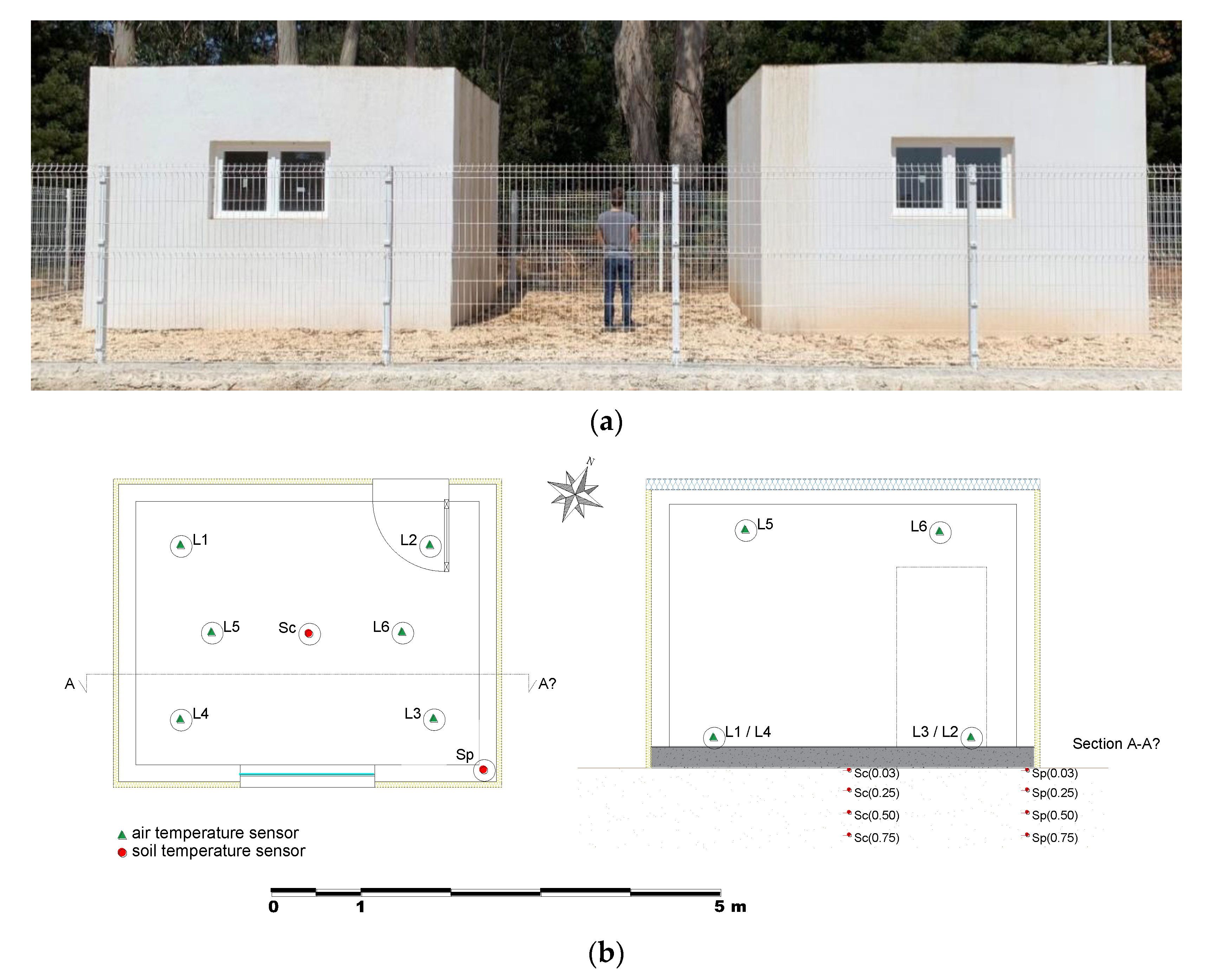
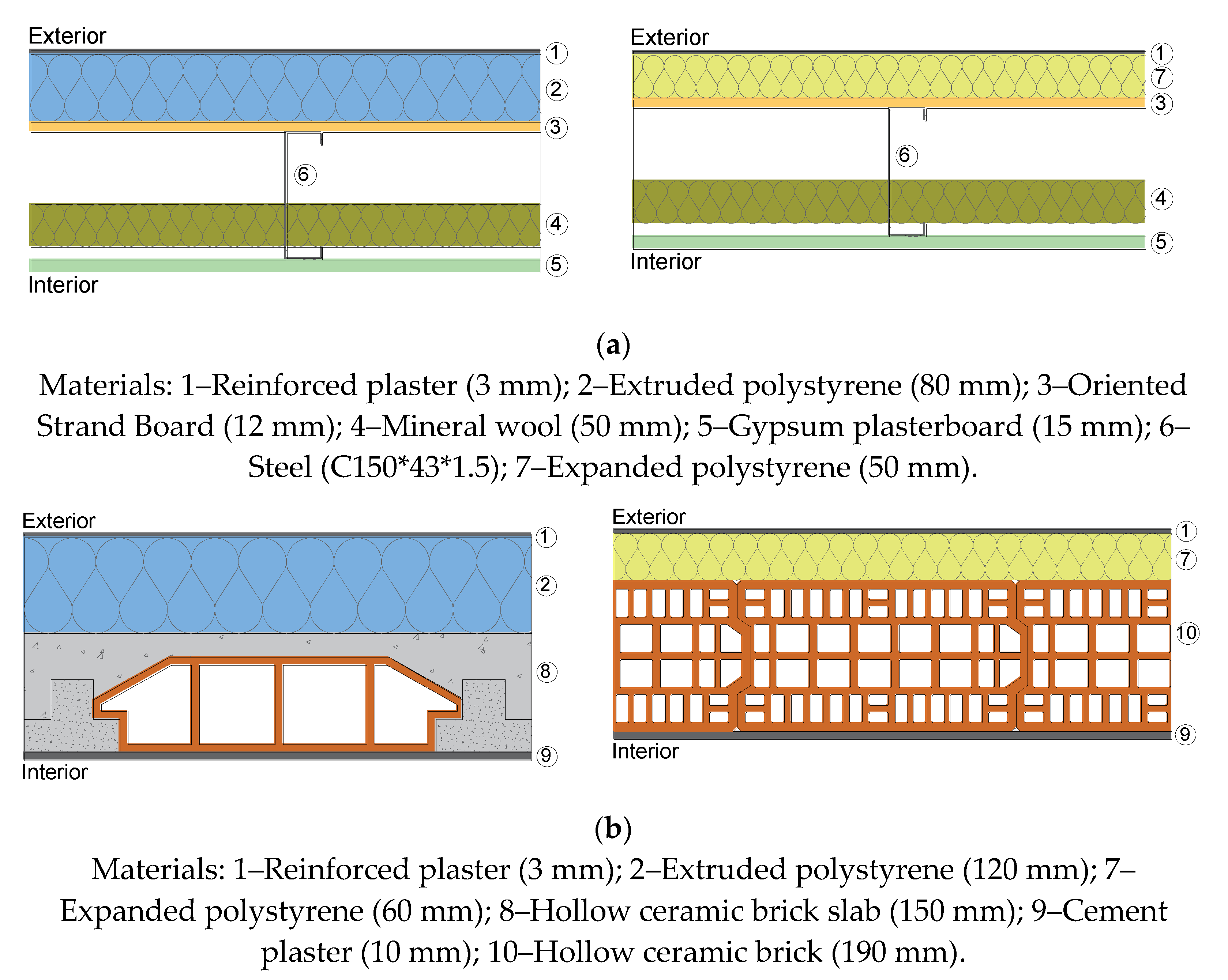
2.2. Experimental Test Cells

The experimental campaign was founded on the construction and monitoring of two identical test cells, differing only by construction system. One was constructed according to the common hollow brick masonry and reinforced concrete construction system (HBM test cell) and the other according to the LSF construction system (LSF test cell).

The test cells were located in Albergaria-a-Velha, in the Aveiro District (central coast region of Portugal, latitude 40°41′23″ N, longitude 08°31′2″ O). This region is characterized by a warm summer Mediterranean climate of Csb, according to the Köppen–Geiger classification [33]. The location is characterised by 1421 heating degree-days (adopting an 18 °C baseline) according to the Portuguese code on the energy performance of buildings [34]. According to the same source, the average value of the solar energy incident on a vertical south-oriented surface during the heating season per unit area is 140 kWh.m⁻².month⁻¹.

The test cells had a regular geometry with inner floor dimensions of 3.87 by 2.97 m and a height of 2.70 m, giving a total interior volume of approximately 31 m³. These significant dimensions were adopted in order to be representative of a real building compartment. Both test cells were ground floor structures that were detached from other structures and had a longitudinal axis roughly along north–south (155° SE). An external view of the test cells is introduced in Figure 1a,b presents a plan view and vertical cross-section, indicating the positions of the different sensors. Complementary information about the case study can be found in [35,36].

Figure 2 presents the configuration and thermal parameters of the opaque construction components. The definition of the opaque elements was driven by the most common solutions applied nowadays in Portugal in residential buildings, leading to the LSF and hollow brick masonry construction. Furthermore, the adoption of these construction solutions also involved consideration of the Portuguese regulations on the energy performance of buildings [34], complying with the limits and requirements for new construction projects in the considered climatic zone.

The walls and roofs were characterized in terms of the internal areal heat capacity (k₁), decrement factor (f), periodic thermal transmittance (Y₁₂), time shift of the periodic thermal transmittance (Δt), and steady-state thermal transmittance (U-value). As shown in

Table 1. Thermal parameters of the external opaque envelope elements.

Thermal Parameters	LSF (Wall)	LSF (Roof)	HBM (Wall)	HBM (Roof)
k1 (kJ.m−2 °C−1)	15.50	16.62	47.26	64.54
f (-)	0.792	0.719	0.130	0.247
Y12 (W.m−2 °C−1)	0.286	0.200	0.047	0.069
Δt (h)	3.20	3.90	8.90	7.30
U-value (W.m−2 °C−1)	0.36	0.28	0.36	0.28

, these elements were characterized by the same U-value but presented different dynamic thermal characteristics, corresponding to distinct levels of global thermal inertia.

The U-values of the construction components were computed considering the procedures presented in ISO 6946 [37] and EN ISO 10211 [38]. The presence of non-homogeneous layers was taken into account in this calculation. ISO 13786 [39] was considered for the calculation of the dynamic thermal parameters.

Introducing significant external thermal insulation rates on the opaque elements leads to a decoupling effect between the internal and external sides of these elements, as stressed by Stazi [11]; therefore, in new, highly insulated structures, the k₁ value assumes a prominent role in managing the heat gains bypassing the external opaque envelope through the glazing and internal gains. On the other hand, the LSF elements showed much lower k₁ values, indicating a smaller capacity of the most inner layers to store and release thermal energy when the indoor temperature varies periodically. Globally, the walls and roofs of the LSF and HBM test cells showed global internal heat capacity rates of 763.54 kJ °C⁻¹ and 2487.41 kJ °C⁻¹, respectively.

Additionally, the lightweight walls and roofs also presented higher f values, which were related to the capacity to delay the incoming or outgoing thermal wave under dynamic conditions; therefore, it can be anticipated that the combination of these two former dynamic parameters makes the LSF test cell more responsive to external environment variations, resulting in more significant fluctuations of the indoor air temperature.

The ground floor slab of each test cell was a 0.23-m-thick reinforced concrete slab coupled to the ground, without thermal insulation, as well as an inner finishing layer. Uninsulated ground floor slabs are frequent in Portuguese residential buildings and are in accordance with the requirements imposed by Portuguese regulations on the energy performance of buildings [34].

Regarding the glazed elements, both test cells had a window with double-pane clear glazing (U-value = 2.8 W m⁻² °C⁻¹; g-value = 0.75) and a wooden frame (U-value = 2.61), presenting an area of 1.50 m² (83% glazed area). The window–floor ratio was defined based on the indications presented in the Portuguese code on the energy performance of buildings [34] to address and mitigate the effects of overheating on energy consumption and indoor thermal comfort. The window–floor ratio of the test cells as approximately 13%.

This small window–floor ratio was used as our aim was to focus the analysis on the construction systems. We intended to isolate the interactions between the external opaque envelope, the outdoor conditions, and the indoor thermal environment. Increasing the window–floor ratio could undesirably diminish the influence of the opaque envelope and hinder this assessment. The same premise was considered to support the construction of detached experimental test cells, allowing maximization of the exposed area of the opaque external envelope, thereby enhancing the influence of the construction system on the indoor thermal environment.

The air permeability of the envelope was evaluated through the blower door test (Retrotec 1000) by calculating the air change rate at a pressure difference of 50 Pa (n₅₀), following the procedure outlined in ISO 9972 [40]. The tests returned airtightness values of 1.0 ± 0.1 h⁻¹ for both test cells, emphasizing the similarities between test cells.

The obtained results were anchored to the design and construction options used for the test cells. Different solutions would provide different results. It would be expected that the differences between test cells would be more notable or less evident depending on the considered solutions in combination with the characteristics of the external environment.

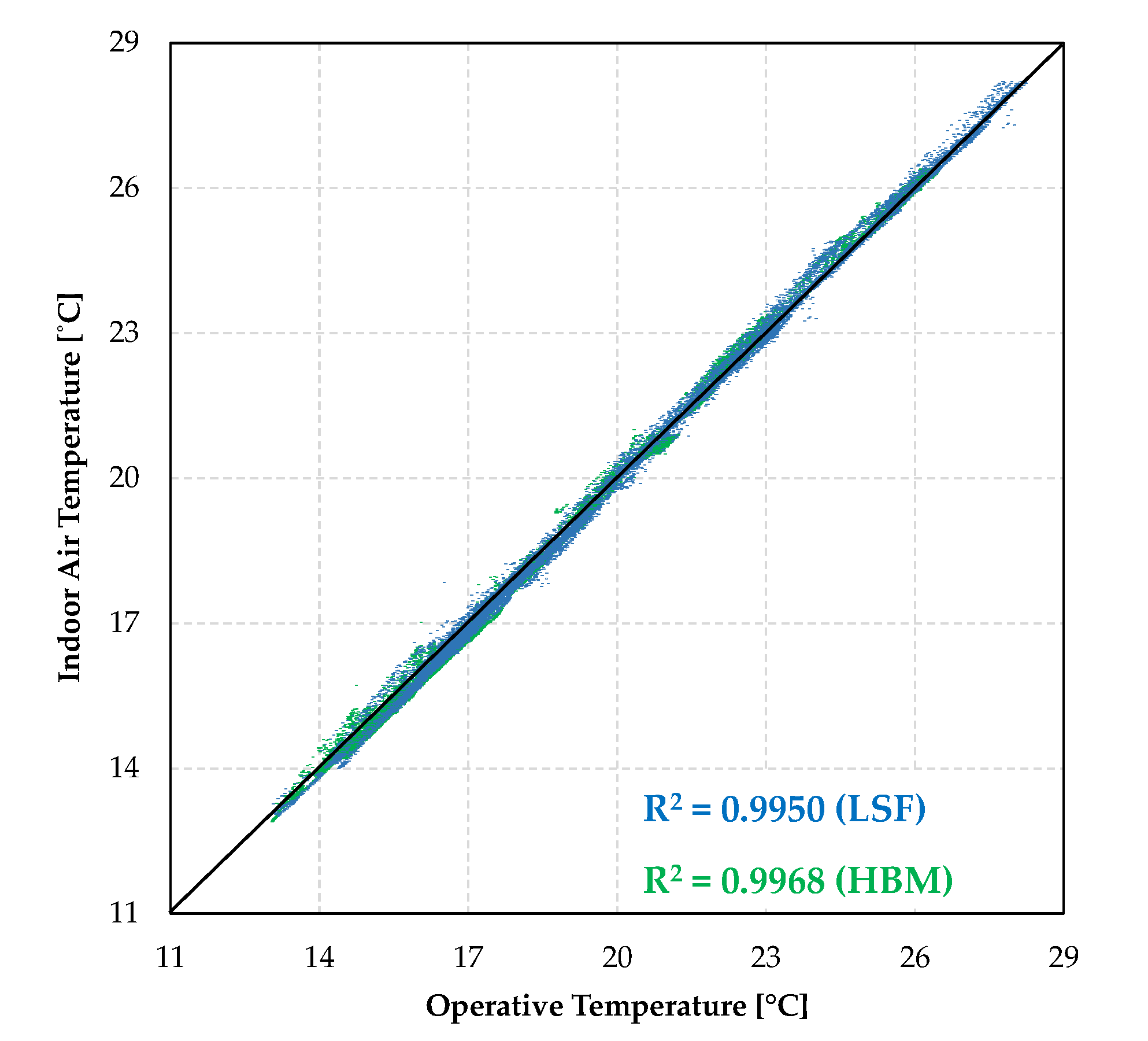
2.3. Indoor Thermal Environment and Thermal Comfort Assessment

The indoor thermal environment of the test cells was studied in two stages: (i) an analysis of the indoor air temperature fluctuation during summer (June–September), the shoulder season (March–May and October), and winter (November–February) over representative weeks; (ii) statistical treatment of the entire monitored period, resulting in graphic representations of the monthly profiles and hourly indoor air temperature profiles for the summer, shoulder season, and winter.

The indoor thermal comfort conditions were evaluated using the adaptive model expressed in EN 16798-1 [41]. The adaptive comfort model was considered due to its high suitability for residential buildings. Generally, in these buildings the opportunities for behavioural adaption in order to avoid discomfort are vast, such as freely adjusting clothing levels or adjusting the metabolic rate. Residential buildings also provide easy access to operable windows and higher control over natural ventilation. Additionally, typical Portuguese residential buildings are naturally ventilated over the year, with heating or cooling systems used according to an intermittent pattern, with reduced usage during more demanding periods of the year.

According to this standard, for buildings defined as category II, the lower and upper limit values of the indoor operative temperature (${\theta }_i$) depend on the running mean outdoor temperature (${\theta }_{rm}$). The indoor comfort of each test cell was assessed using two different procedures, based on the “percentage outside the range” and “degree hours criteria” methods outlined in EN 16798-2 [42]. The former quantifies the percentage of time that the indoor air temperature is outside the thermal comfort range. For the latter, the accumulated difference between the indoor air temperature outside the range and the comfort limit is quantified. This difference is divided by the number of time steps for a given period, translating the average difference per time step between the indoor air temperature and comfort conditions. This procedure resulted in the indicator designated here as the average discomfort index (ADI), which was calculated according to Equation (1) for each of the considered discomfort zones.

$$ADI=\frac{{\sum }_{i=1}^N|{\theta }_i-{\theta }_{limit\left(lower, upper\right)i}|}{N}\left[{ }^{°}\mathrm{C}\right]$$

(1)

when,

$$({\theta }_i<{\theta }_{limit\left(lower\right)i}\mathrm{or} {\theta }_i>{\theta }_{limit\left(upper\right)i})$$

where, θ_I is the indoor air temperature (°C); ${\theta }_{limit\left(lower, upper\right)i}$ is the comfort limit value of the indoor air temperature (°C); N is the number of time steps (-).

In the present work, the operative air temperature was considered to be equal to the indoor air temperature. The operative temperature was calculated and correlated with the indoor air temperature considering the entire monitoring period to substantiate this premise. Figure 3 presents the obtained results for each test cell. The mean radiant temperature of each test cell was calculated from the measured surface temperatures of all eight inner surfaces, following the procedures suggested in the ASHRAE Handbook—Fundamentals [43]. The operative temperature was computed according to the indications expressed in ASHRAE Standard 55 [44].

To further support and illustrate the previous assumption, the indoor air temperatures for each experimental test cell over representative summer and winter weeks are presented in Figure 4. The indoor thermal environments during these periods are analysed in more detail in Section 3. In the presented images, the surface temperatures of the walls, slabs, and roofs of the test cells are also shown.

As can be seen from Figure 4, the surface temperatures of the construction elements of each test cell almost perfectly overlap with the indoor air temperature, supporting the proximity between the indoor air and radiant temperatures of the surfaces.

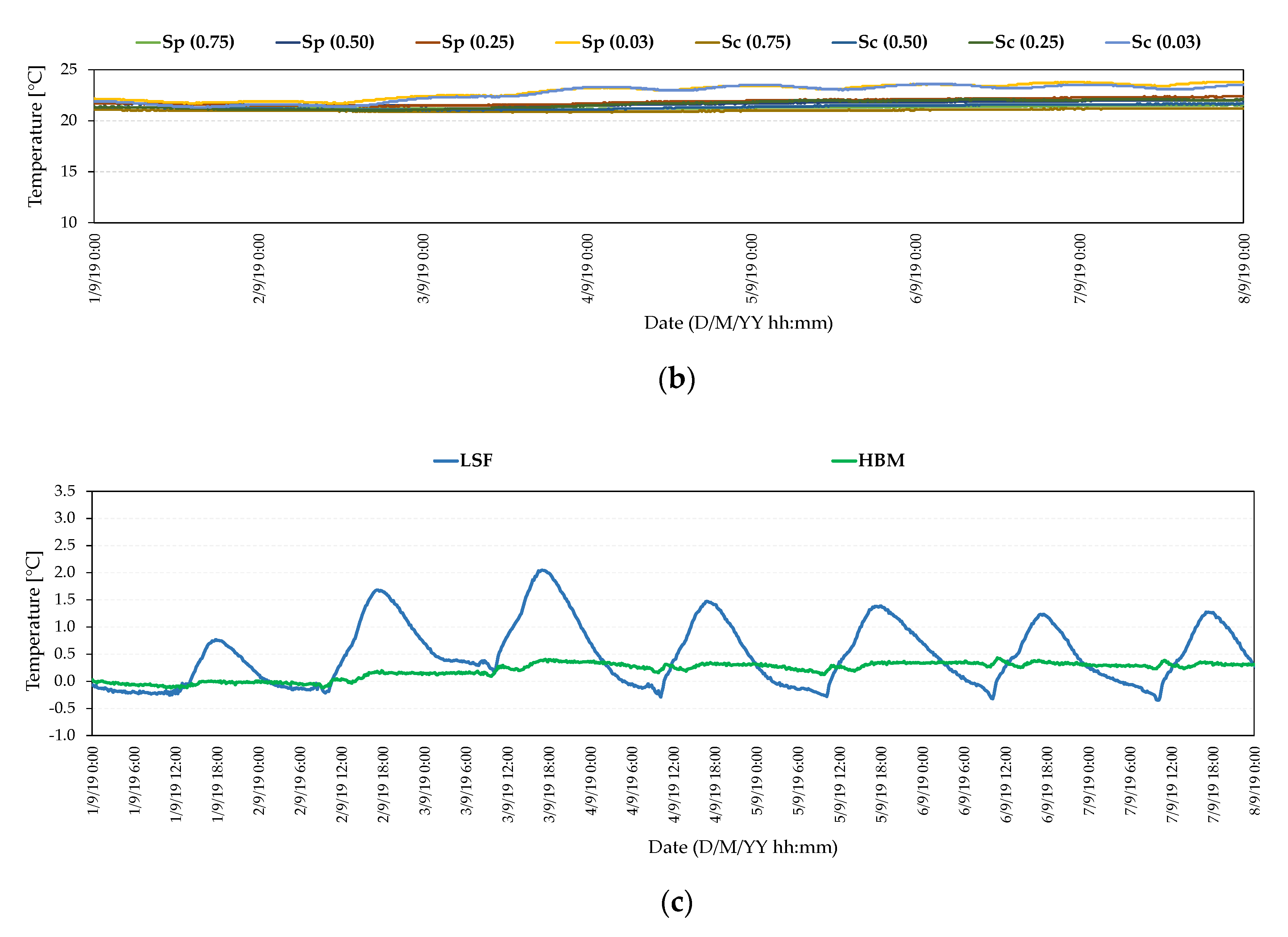
2.4. Soil Temperature

Since a significant percentage of the interior surface area of the test cells is in contact with the ground (approximately 20%) and acknowledging the influence of the soil temperature throughout the year on the indoor thermal environment of ground floor structures, this parameter was also monitored under the LSF test cell at different depths and locations. The monitoring was carried out under the LSF test cell because this is the type of structure that is the main focus of this work.

Data regarding soil temperatures at different depths can be found in climatic files or even using analytical formulas, such as Kasuda’s formula [45]; however, these temperatures refer to “undisturbed” soil, which could significantly differ from the soil temperature under a building site.

2.5. Monitoring Equipment

The measurements and monitoring conditions considered in the present work were carried out according to ISO 7726 [46]. All measured data were collected at 10 min intervals. A data logger and several sensors were used:

• Outdoor environmental conditions (data logger: data collected using two ICP I-7015P input modules and two I-7561 modules):
  • A weather station with the following sensors:

    -

    LP PYRA03AC pyranometer, measuring the global horizontal radiation (accuracy: ±5 W/m²);

    -

    DeltaOHM HD9007-A1 thermohygrometer, including a double anti-radiation shield (accuracy: ±0.1 °C and ±2% HR).

  • Soil temperature—PT100 temperature probes were distributed at two different locations under the concrete slab of the LSF test cell, according to the schematic layout presented in Figure 1b. One location was under the centre of the slab (Sc) and the other on the periphery (Sp). Each location comprised four monitoring depths (0.03, 0.25, 0.50, and 0.75 m).
• Indoor environmental conditions:
  • Indoor air temperature—SHT31 temperature and relative humidity sensors (accuracy: ±0.3 °C and ±2% HR) were allfgiocated according to the schematic layout presented in Figure 1b. The sensors were distributed among an inferior level (0.1 m from the ground floor slab) and a superior level (2.4 m from the slab).
  • Surface temperature—Type K thermocouples were used, whereby one thermocouple was placed in the centre of each interior surface.

3. Results and Discussion

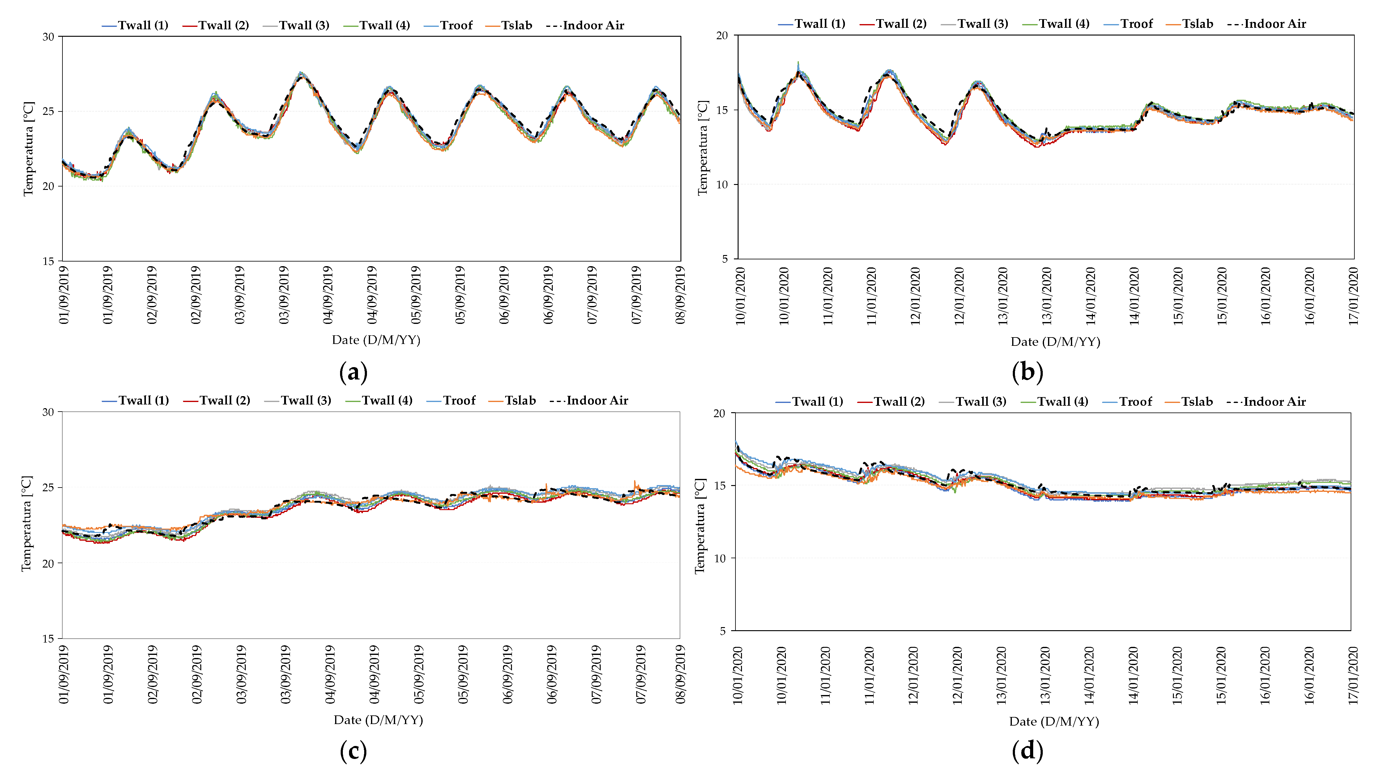
3.1. Indoor Thermal Environment—Representative Summer, Shoulder Season, and Winter Weeks

In this section, the obtained results concerning the indoor thermal environment are presented and discussed. The indoor air temperature profiles for representative summer, shoulder season, and winter weeks were analysed. For each test cell, the temperature profiles corresponded to the average value between the monitoring levels (near the floor slab and the ceiling). For each monitoring level, the average value for the different sensors was calculated.

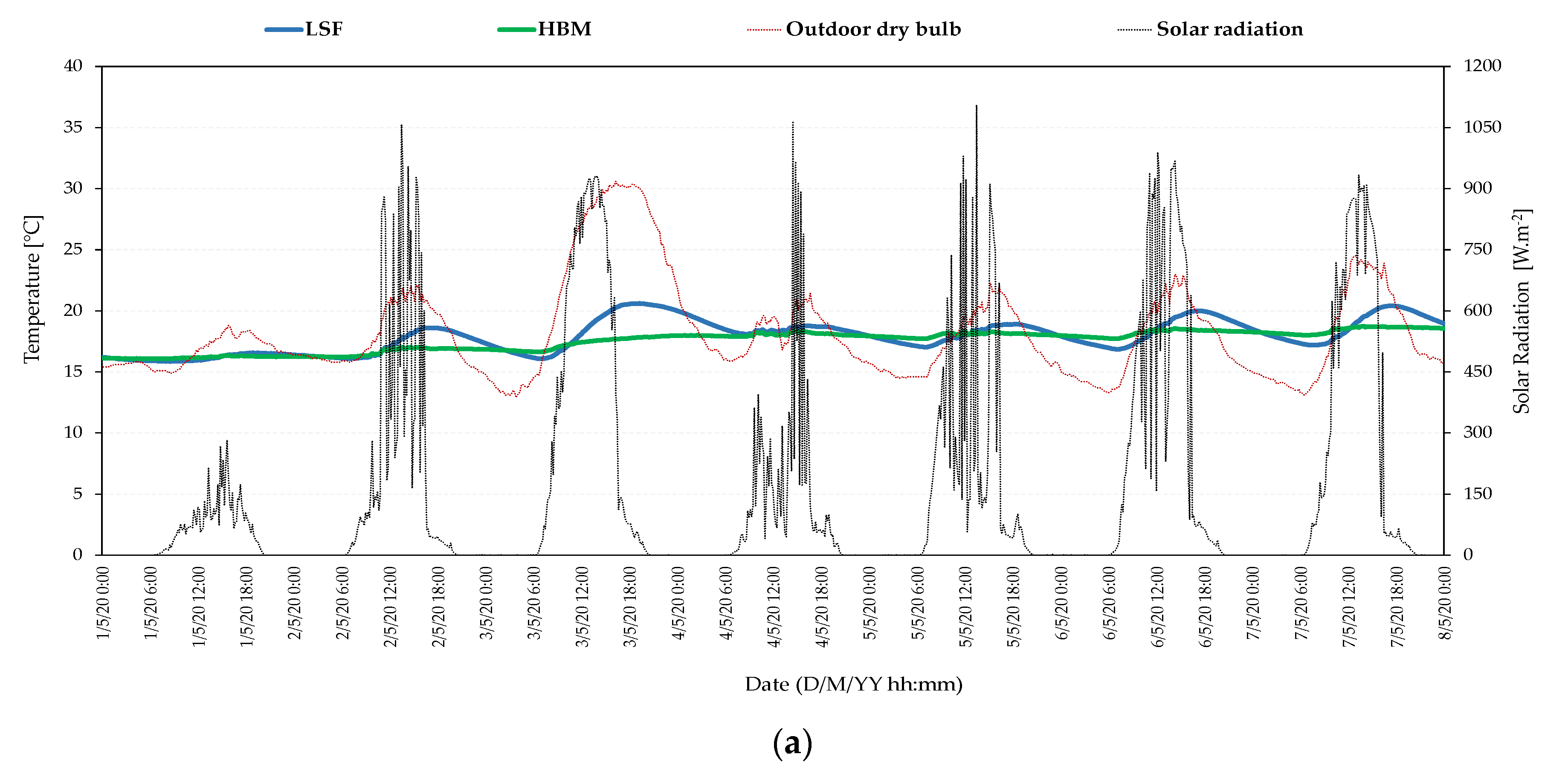
• Representative Summer Week

The week of 1–8 September was selected to discuss the summer season. The chosen week was characterised by intense solar radiation from clear sunny days (reaching values above 900 W m⁻²), significant maximum outdoor dry bulb temperatures, and considerable daily temperature fluctuations (variations up to nearly 20 °C), as can be seen in Figure 5a. The analysed week presented a noteworthy outdoor dry bulb temperature fluctuation, highlighting the role of thermal mass in this dynamic behaviour.

Figure 5a also presents the indoor air temperature fluctuations in both test cells during the summer week. The difference in indoor daily temperature amplitude and the magnitude of the maximum and minimum values is evident when comparing the two test cells. It can be seen that the indoor air temperature in the HBM test cell remained practically constant with respect to the daily fluctuation of the outdoor dry bulb and with slight variations over the analysed summer week, differing from the LSF test cell. Additionally, the latter presented more expressive peak values for the maximum and minimum registered indoor air temperatures, with more relevance regarding the maximum temperatures. In fact, the differences in terms of minimum temperatures were not noteworthy. The greatest difference between test cells was registered on September 3rd, when the daily outdoor dry bulb temperature amplitude was more meaningful and the highest diurnal temperature peak was registered, showing the differences in and role of thermal mass. On this day, a peak difference between test cells of approximately 3.3 °C was registered.

The more volatile behaviour of lightweight structures, more closely following outdoor environmental conditions, has been reported across different research studies [27,28,29,30,31]. It has been shown that higher indoor air temperature fluctuations occur in lightweight structures, resulting in more considerable maximum and minimum temperature values. The use of appropriate thermal mass levels is widely suggested as an efficient design strategy to attenuate or mitigate this behaviour and improve indoor thermal comfort.

The benefits of thermal mass are clear in warmer climates, as demonstrated by Ogoli [30]. Gregory et al. [31] also stressed the beneficial contribution of thermal mass during the summer to residential construction performance in the warm Australian climate. It has been shown that in such demanding environments, construction solutions with higher k₁ values provide important advantages over lightweight solutions.

The differences between test cells were primarily due to the much higher k₁ values of the HBM test cell, significantly contributing to temperature peaks and daily temperature stabilization. On the other hand, in the LSF test cell, heat dispersion and storage capacity in the inner layers were more reduced, which translated into more pronounced indoor temperature build-up. Additionally, by presenting a higher f value, the LSF test cell showed its lower capacity to mitigate the incoming thermal waves, contributing to the higher heating rate of the indoor air. The experimental study conduct by Givoni [29] in the warm climate of California also underlined the differences in terms of thermal mass, which can significantly influence the response to solar heat gains in terms of the maximum indoor air temperature build-up rate values. Besides presenting significantly different heating rates, it can also be observed in Figure 5a that the indoor air temperatures in each test cell also showed very different cooling rates during the colder period of the daily cycle. The HBM test cell consistently reveals a much lower cooling rate compared with the LSF test cell. The indoor air temperature in the LSF test cell showed a cooling of approximately 4.5 °C between the maximum peak temperature on September 3rd and the minimum temperature on September 4th after night cooling. The indoor air temperature in the HBM test cell only cooled down by around 0.5 °C over the same period. The combined effect of three factors can explain the different night cooling rates between the test cells. First, the temperature gradient between the indoor air and the soil was higher in the LSF test cell, leading to a higher heat exchange rate. Secondly, the LSF test cell presented a lower k₁ value, meaning not as much heat was stored in the inner layers to balance night cooling. Finally, this cell presented a higher f value, and consequently a poorer capacity to mitigate the outgoing thermal wave. In the study by Gregory et al. [31], the indoor cooling potential during the night was also noted.

Figure 5b reveals how the contact with the ground, through the uninsulated slab, can benefit the indoor thermal environment of the LSF test cell during the cooling season. Despite the significant fluctuation of the outdoor dry bulb temperature over the period under analysis, the soil temperatures at the different monitoring positions and depths were practically constant. Ranging intervals of approximately 1.5 °C for the two deepest monitoring positions (0.50 m to 0.75 m) and 2 °C for the most superficial position (0.03 m) were registered, which were more influenced by the indoor air temperature. Besides the low fluctuation, the soil temperature was also close to the summer comfort temperature range [42]. Given the more responsive behaviour to the outdoor stimulus of the LSF test cell, being more prone to overheating and temperature fluctuations, the contact with the ground plays a role in regulating the indoor air temperature at levels closer to the comfort range, acting as an important passive cooling element. The purpose of Figure 5b is to provide a qualitative overview of the soil temperature to complement the discussion of the thermal behaviours of the test cells, rather than providing an extensive analysis of the temperatures at the different positions.

Figure 5c presents the indoor air temperature stratification of the two test cells. The presented values correspond to the temperature differences between the average values for the different sensors located at the superior level and the average values for the sensors positioned at the inferior level. As expected, both cells registered higher indoor air temperatures at the superior monitoring level during the vast majority of the time. The stratification was more evident in the LSF test cell and during the central hours of the day, when differences of up to near 1.5 °C were registered between the inferior and superior levels (0.1 m and 2.4 m from the slab, respectively). On the other hand, the temperature stratification for the HBM cell was only modest, with a maximum value of approximately 0.5 °C. Regarding local discomfort, the maximum vertical air temperature difference between the head and ankles should be less than 3 °C according to ISO 7730 [47]. The maximum vertical difference between 0.1 and 2.4 m levels found in the cells was 2 °C, verifying this condition.

The registered differences between the two cells may be supported by the different thermodynamic characteristics of the most internal construction layers and by the magnitude of the indoor air temperature in each cell. The lower thermal diffusivity and thermal mass of the inner layer of the LSF components do not favour heat dissipation towards the walls and or heat storage, thereby resulting in temperature stratification. Additionally, the LSF cell presented higher indoor air temperatures, especially during the warmer period of the day. The presence of a colder element (slab) at an inferior construction level, when compared with the average indoor air temperature, favours vertical convective currents inside the LSF cell.

• Representative Shoulder Season Week

The week of 1–7 May was analysed as a shoulder season week. The selected week was characterised by mild outdoor dry bulb temperatures, ranging during most of this period from approximately 13 °C to 24 °C, as well as moderate daily fluctuations (up to approximately 11 °C), as can be seen in Figure 6a. High solar radiation was for every monitored day (predominantly around 900 W m⁻²), although with a marked intermittent character. An atypical day (3 May) was also noted when the outdoor dry bulb temperature reached a more elevated value (approximately 30 °C) and consequently a more marked daily amplitude (approximately 17 °C).

The fluctuations of the indoor air temperature over the analysed shoulder season week are shown in Figure 6a for both test cells. It can be noticed that the differences between test cells were not as noticeable in the summer. In this week, the outdoor environmental conditions were not as dynamic as in the previous analysis, meaning that the daily outdoor dry bulb temperature expression, in terms of the amplitude and magnitude of peak values, was not as meaningful. Consequently, the dynamic behaviour of the thermal mass was less exploited and the differences between the two test cells were less noteworthy.

Ignoring 3 May, maximum daily indoor temperature amplitudes of approximately 0.7 °C and 3.2 °C were measured for the HBM and LSF test cells, respectively. Similarly to the results verified for the summer week, the registered differences between test cells were more evident in terms of maximum daily temperatures. The maximum measured difference between test cells after night cooling was below 1 °C.

The impact of thermal inertia was clearly visible on May 3rd, corresponding to the day with higher outdoor dry bulb temperatures. On this day, the indoor air temperatures of the two test cells showed a maximum difference of approximately 2.8 °C. The LSF test cell promptly responded to the sudden increase in the outdoor dry bulb temperature, which triggered a significant increase in the indoor air temperature. On the other hand, the HBM test cell benefited from higher thermal inertia in buffering the instant effects of the atypical warmer day. Over the shoulder season week, total indoor air temperature fluctuations of approximately 4.8 °C and 2.6 °C were measured in the LSF and HBM test cells, respectively.

Figure 6b reveals the remarkable stability of the soil temperature during the shoulder season week. A temperature amplitude of approximately 2.3 °C was measured over the week for the most superficial monitoring locations (0.03 m). For the second most superficial positions (0.25 m), the measured amplitude decreased to nearly 1.5 °C, which was similar to the temperature amplitude registered for these positions during the summer week.

The indoor vertical temperature stratification of the two test cells during the shoulder season week is presented in Figure 6c. The measured stratification results were again higher for the LSF test cell, whereas the HBM test cell revealed a notably homogeneous indoor thermal environment. A stratification result of nearly 3.1 °C was registered in the LSF test cell during the warmer hours of the day on 3 May. This value was greater than the measurements shown for the summer week, even for days with notably higher outdoor dry bulb temperatures. Acknowledging that a wide array of factors may contribute to such situations, one reason may be the increased daily outdoor dry bulb amplitude rate, which was significantly higher on 3 May than on any other day during the summer week. The rapid indoor air temperature build-up in the LSF test cell, associated with the lower capacity to store heat in the inner layers of the construction components, catalysed the vertical stratification.

The maximum measured vertical stratification in the LSF test cell exceeded the 3 °C limit stressed in ISO 7730 at some points of the day [47], which is often associated with local discomfort due to vertical temperature differences; however, ISO 7730 relates to the distance between the head and ankles, which is inferior to the vertical distance considered here (2.3 m).

• Representative Winter Week

The winter week (10–17 January) was divided into two different periods in terms of outdoor environmental conditions, as shown in Figure 7a. The first period (between 10 and 13 January) was characterized by moderate solar radiation (predominantly under 450 W m⁻²), low minimum outdoor dry bulb temperatures, and considerable daily outdoor dry bulb fluctuations (with variations exceeding 10 °C). After a transition phase, a different period was observed (between 14 and 17 January), characterized by periods with lower and intermittent solar radiation, and consequently a more stable outdoor dry bulb temperature.

Figure 7a shows the fluctuations in indoor air temperature for both test cells during the winter week. During the first half of the week (10–13 January), when more dynamic outdoor conditions were registered, the two test cells revealed different indoor temperature profiles. Similar to the summer analysis, the LSF test cells presented higher daily indoor temperature fluctuations and more expressive maximum and minimum values, more closely following the outdoor dry bulb temperature variations. In turn, the HBM test cell registered less variation over the daily cycle. The different heating and cooling rates and indoor temperature profiles for each test cell are supported by the same governing factors previously exposed in the summer analysis.

The registered differences between test cells during the winter week are more evident in terms of the magnitude of the daily temperature fluctuations in indoor air temperature rather than in terms of the absolute differences between the maximum and minimum values. The maximum diurnal peak difference between test cells was approximately 1 °C on 11 January and the maximum difference after cooling was approximately 1.9 °C on 12 January.

Typically, during the winter, even in Southern European climates, one of the main requirements is for thermal insulation, reducing heat losses as much as possible. As such, the f value and especially the U-value are common indicators used to express winter performance; however, considering that the test cells have no active heating or cooling systems, being heated only by solar gains, the k₁ value also plays an important role, contributing to the stabilization of the indoor air temperature due to more efficient management of the solar heat gains during a daily cycle.

For the second period of the winter week, different thermal behaviour was observed. During this period, the intensity of the solar radiation was lower and more intermittent throughout the day. The outdoor dry bulb temperature profile showed more stationary behaviour. In such periods, there were very small differences between the two test cells. The absence of significant outdoor dry bulb temperature fluctuations did not allow for the dynamic behaviour of the thermal mass to be exploited. During this period, both test cells revealed indoor air temperatures close to the outdoor dry bulb temperature, given the absence of significant energy gains. In between these two periods, the higher inertia of the HBM test cell allowed for higher indoor air temperatures to be attained.

The obtained results were in line with the findings achieved by Gregory et al. [31] during a mild Australian winter. The authors observed that the indoor thermal environments of the analysed lightweight and heavyweight construction types during the winter months were similar. They also stressed that the indoor air temperatures in the analysed structures were higher than the outdoor temperatures, regardless of the level of thermal mass, which was also in accordance with Figure 7a. The greenhouse effect and good thermal quality of the external opaque envelope were presented as causes for this scenario.

Figure 7b presents the soil temperatures during the representative winter week. In contrast to the summer week, the benefits from the contact with the ground were not so evident. The soil temperatures in the different monitoring positions remained practically constant, although with colder temperatures (ranging from approximately 14 °C to 16 °C); however, regardless of the stability over time, the presented temperatures were inferior to winter comfort temperatures [42]. Despite the soil temperatures being higher than the outdoor temperatures for the vast majority of the week, there was no thermal insulation on the ground floor, which may have led to significant heat loss towards the ground. Nevertheless, from the obtained results, it can be concluded that it would be more beneficial to have the ground slab in contact with the soil rather than exposed to the outdoor dry bulb temperature, as would be in the case with a ventilated crawl space.

Figure 7c introduces the indoor vertical temperature stratification of the two test cells during the winter week. The stratification remained visible during the winter week, with maximum values of near 1.5 °C and 1 °C for the LSF and HBM test cells, respectively. The magnitude of the vertical stratification values also differed in first and second periods of the week. During the first period, the stratification was more significant, especially in the LSF test cell. During the second period, the magnitude of this effect was less evident. Additionally, the soil and indoor air temperatures were similar, meaning that the slab also presented similar temperatures, reducing the vertical convective currents mentioned for the summer period; therefore, the criteria regarding the maximum vertical air temperature difference expressed in ISO 7730 [47] to avoid discomfort was not exceeded.

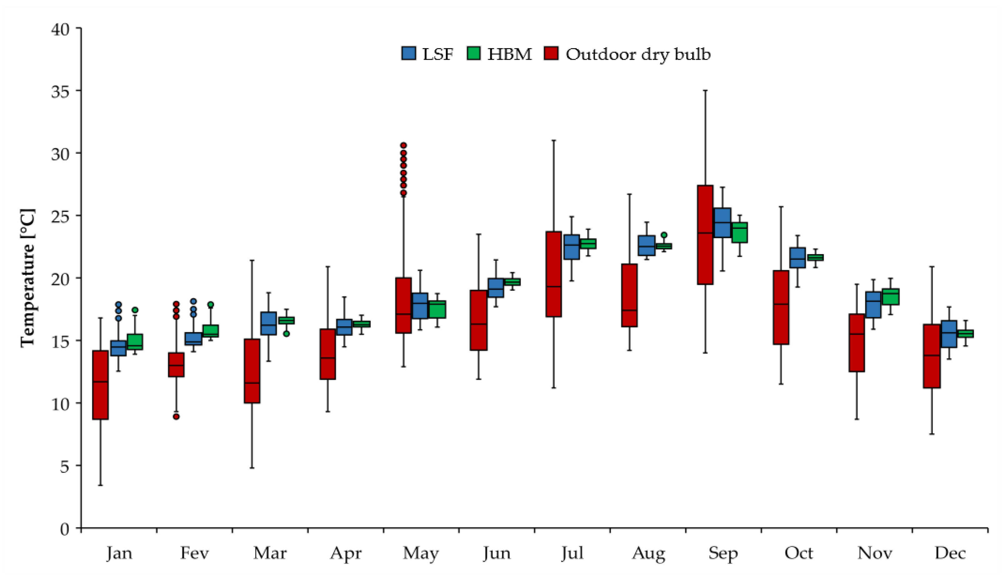
3.2. Indoor Thermal Environment—Annual and Daily Temperature Profiles

In order to provide a global overview of the complete monitored period, the measurements obtained during the twelve months were statistically analysed. In this section, the annual and daily air temperature profiles of each test cell are presented and discussed. While the former provides a more general approach, the latter allows more detailed analysis on a smaller scale.

• Annual Indoor Air Temperature Profile

Figure 8 shows a monthly box plot representation of the indoor air temperature for each test cell, as well as the outdoor dry bulb temperatures. The first aspect to be highlighted is the range of indoor air temperature fluctuations throughout the year compared with the outdoor dry bulb temperature amplitude. Additionally, was also verified that the monthly box plots of both test cells primarily comprised median values of the outdoor dry bulb temperatures and the associated maximum values. Due to the good thermal quality of the external envelope of the test cells and low air permeability, heat was better conserved inside the test cells, resulting in the above behaviour.

From the analysis shown in Figure 8, we noted that in general terms, the differences between the test cells in the statistical analysis were not as evident as they were in the previous section, especially in terms of median values. The monthly median values were quite identical in every monitored month, with the differences always inferior to 1 °C. As the analysis was performed less broadly, the differences between the test cells were more evident. The interquartile range dimensions of the box plots revealed a wider amplitude of indoor air temperatures for the LSF test cell, stressing the more marked fluctuations in indoor thermal conditions in this test cell over the monthly periods. The most significant disparities between test cells were related to the maximum and minimum monthly temperature values, which were up to 2.5 °C.

• Daily Indoor Air Temperature Profiles—Seasonal Representation

Figure 9 shows details of the analysis by presenting the daily indoor air temperature profiles for the entire monitored period. The total period was divided into the three previously considered periods of the year, namely the summer, shoulder season, and winter. Figure 9a–c presents these profiles for the considered periods in the same order.

Regarding the summer months, Figure 9a reveals a predominance of higher and more meaningful maximum peak temperatures in the LSF test cell, which is especially evident during the mid-afternoon. The registered differences are a clear indicator of the differences in terms of the thermal inertia and consequent dynamic behaviour of the test cells.

A maximum indoor air temperature of 27.25 °C was registered in the LSF test cell, occurring in the period between 16:00 and 17:00. The maximum value measured in the HBM test cell equalled 25.02 °C, which registered earlier, between 13:00 and 14:00. The minimum registered temperature in the LSF test cell was 17.70 °C, occurring between 08:00 and 09:00. The HBM test cell gave the minimum measured temperature for the period between 07:00 and 08:00, with a value of 19.04 °C; therefore, over the analysed summer period, the indoor air temperature in the LSF test cell was within a range of 9.55 °C, while in the HBM test cell the indoor air temperature varied within a range of 5.98 °C.

Analysis of Figure 5a and Figure 9a regarding the summer season verifies that the maximum daily indoor air temperature peak was typically registered first in the HBM test cell; therefore, the premise that a building with low thermal inertia presents the maximum indoor air temperature peak earlier than a high thermal inertia building and with a higher magnitude was only partially verified by the presented results obtained under real free-running boundary conditions.

During the period from 15:00 to 16:00, the largest hourly amplitudes of indoor air temperature were measured in both cells. In this hourly time slot, the LSF and HBM test cells showed temperature ranges of 8.18 °C and 5.30 °C, respectively.

The analysis of the shoulder season months represented in Figure 9b extended the behaviour and patterns verified for the summer months. Once again, the effects triggered by the differences in the dynamic responses of the test cells were evident in terms of indoor air temperature fluctuations and maximum and minimum peak measured values.

Maximum indoor air temperature values of 23.38 °C and 21.90 °C were measured for the LSF and HBM test cells during the shoulder season months, respectively. In terms of the minimum indoor air temperatures, values of 13.34 °C for the LSF test cell and 15.50 °C for the HBM test cell were measured; thus, over the analysed shoulder season period, the indoor air temperatures in the LSF test cell varied within a range of 10.04 °C, while in the HBM test cell the indoor air temperatures varied within a range of 6.40 °C range.

The expression of the median values over the daily cycle followed the same behaviour that was verified for the summer months. There was a predominance of higher indoor air temperatures in the LSF test cell from the first hours of the afternoon until the end of the daily cycle, with higher median values for each hourly period. Conversely, the closer response to the nocturnal temperature drop from the LSF test cell showed a predominance of colder indoor air temperatures during the nocturnal and morning periods.

Lastly, regarding the winter months analysis, Figure 9c reveals a different scenario from the previous analysis for the summer and shoulder season months. The predominance of higher indoor air temperatures during a significant part of the daily cycle and higher maximum temperatures for the LSF test cell was statistically not as obvious during the winter period.

Figure 9c shows that the LSF test cell benefited from the more responsive behaviour to the outdoor environmental conditions during the winter months during some periods of the day. Predominantly, the indoor thermal environment in the LSF test cell outperformed the HBM test cell during the afternoon period, when warmer outdoor environmental conditions were registered, as also shown in Figure 7a. For this period, the hourly box plots of the LSF test cell present higher median values; however, the minimum hourly indoor air temperatures were lower when compared with the HBM test cell. The maximum hourly temperatures were similar for both test cells during the afternoon period.

By the final hours of the evening period, the lower thermal inertia of the LSF triggered a closer response to the outdoor dry bulb temperature drop. As the nocturnal period advanced, the indoor air temperature of the LSF test cell more clearly indicated inferior indoor thermal environment compared with the HBM test cell, with lower peak and median hourly values. This scenario was maintained until the first hours of the afternoon period of the next day.

Zhu et al. [28] described a significantly better scenario for construction with high thermal mass during the heating season, which in general terms is in line with the obtained results; however, it shall be noticed that in their study, the environmental conditions were very different from the present study, enhancing the benefits of the thermal mass.

Maximum indoor air temperature value of 19.87 °C and 19.97 °C were measured for the LSF and HBM test cells during the winter months, respectively. In terms of the minimum indoor air temperatures, values of 12.53 °C for the LSF test cell and 13.90 °C for the HBM test cell were measured; therefore, over the analysed winter period, the indoor air temperature in the LSF test cell varied within a range of 7.34 °C, while in the HBM test cell the indoor air temperature varied within a range of 6.07 °C.

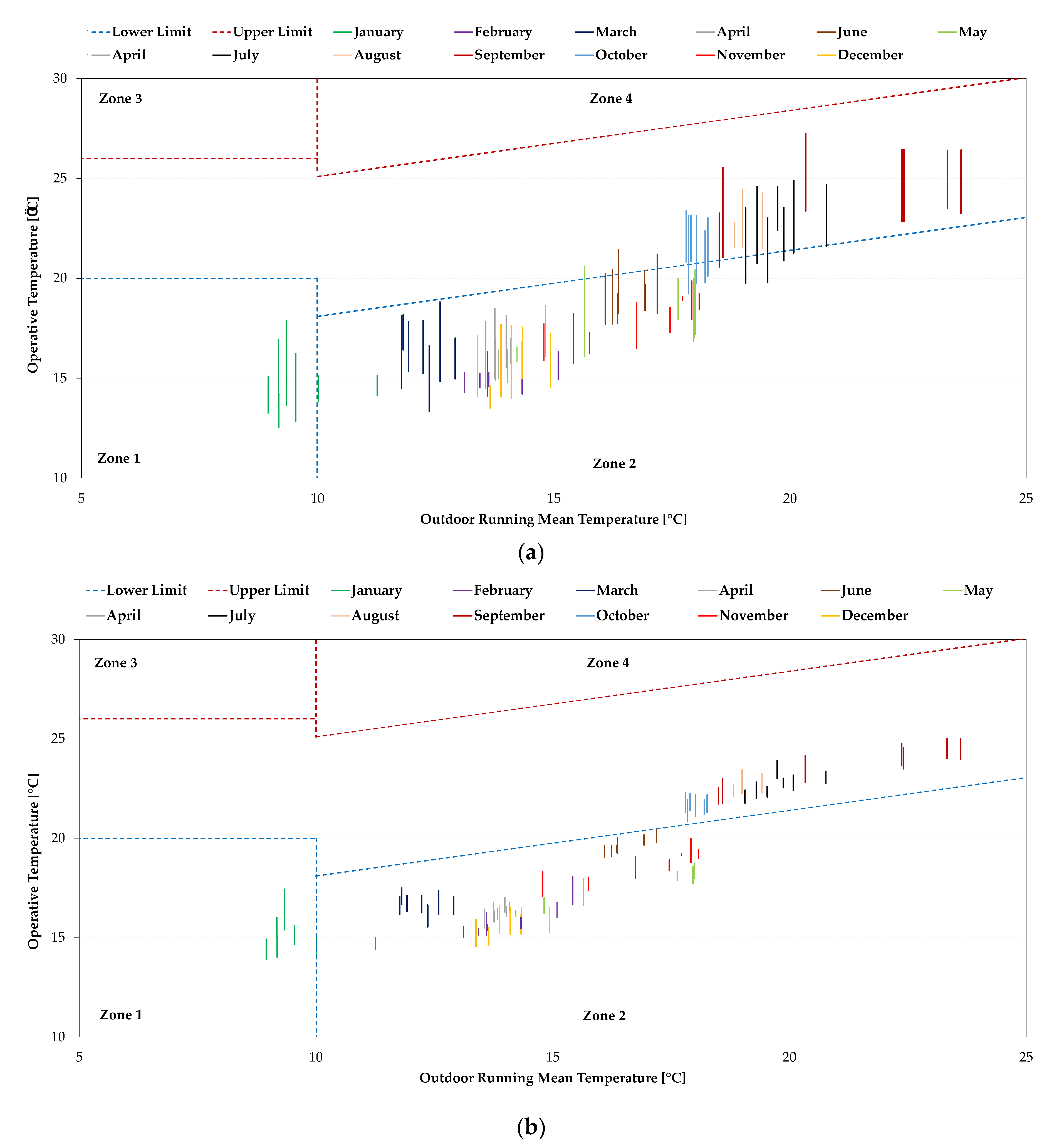
3.3. Indoor Thermal Comfort

In this section, the indoor thermal comfort levels of both test cells during the monitoring period are presented and discussed. The methodology proposed in EN 16798-1 [41] and EN 16798-2 [42] is considered for the thermal comfort evaluation.

The obtained results are graphically presented in Figure 10. The upper and lower limits of comfort are defined according to EN 16798-1 [41] and the daily indoor temperature range of each test cell are shown, illustrated by the scattered plot results for each monitored 10 min interval data. In this analysis, four discomfort zones were considered. Zones 1 and 2 corresponded to discomfort regions under the lower limit of comfort and zones 3 and 4 were related to discomfort regions above the defined upper limit. The first two zones defined the overcooling region, while the last two were associated with overheating. This aim of this division was to further detail each discomfort region, allowing better characterization of the behaviour of the test cells.

The first aspect that can be immediately highlighted Figure 10 is the predominance of an overcooling scenario for both test cells. Additionally, a significant part of the registered discomfort caused by overcooling can be seen in zone 1, indicating severe discomfort.

Both test cells spent the vast majority of the time within the comfort range during the summer months, except in June. During this time, some overcooling periods were registered for both test cells; however, in addition to having a smaller expression (except for June), these periods were within zone 2 of overcooling, which may have inferior relevance during the warmer months. Despite presenting an overall comfortable indoor thermal environment during the warmer months, the LSF test cell closely approached the upper limit of comfort during September, indicating possible overheating scenarios in cases of more demanding outdoor environmental conditions. Additionally, the presence of internal gains would also be an important factor that would aggravate the overheating risk in the LSF test cell, as demonstrated in a previous on considering experimental test cells [35]. On the other hand, this study has demonstrated that internal gains provide an important beneficial contribution, improving the indoor thermal environment of the LSF test cell and reducing thermal discomfort.

To further assess the indoor thermal comfort levels of both test cells, it was important to quantify the duration and magnitude of the discomfort periods.

Table 2. Thermal comfort evaluation based on the percentage of hours of overcooling (%OCh) and average discomfort index (ADI) indicators.

Test Cell	Indicator		Jan	Feb	Mar	Apr	May	Jun	Jul	Aug	Sep	Oct	Nov	Dec
LSF	% OCh	Zone 1	71	-	-	-	-	-	-	-	-	-	-	-
		Zone 2	29	100	100	100	95	84	22	12	4	24	100	100
	ADI		5.03	4.23	3.75	3.21	2.38	1.13	0.13	0.06	0.01	0.14	2.49	3.86
HBM	% OCh	Zone 1	71	-	-	-	-	-	-	-	-	-	-	-
		Zone 2	29	100	100	100	100	100	-	-	-	-	100	100
	ADI		4.62	3.67	3.48	3.09	2.74	0.58	-	-	-	-	1.9	3.93

summarizes the obtained results from the comfort analyses based on the “percentage outside the range” and “degree hours criteria” methods prescribed by EN 16798-2 [42]. The percentage of hours of overcooling (%OCh) and average discomfort index (ADI) results are presented for each month. The results from the two considered methods should be interpreted in relation to each other.

It can be seen that in general terms, the LSF test cell presents more discomfort hours and a higher magnitude of discomfort during the monitored period.

Table 2 shows that the two test cells present the same scenario during the winter months of the monitored period in terms of the percentage of hours of discomfort, primarily in zone 1. The differences are more noticeable in terms of the ADI. This indicator points to the HBM test cell as being less uncomfortable during November, January, and February by 0.59 °C, 0.37 °C, and 0.56 °C, respectively. The LSF test cell presents a lower ADI value for December, with a slight difference of 0.07 °C.

Contrasting with the winter months, the comfort analyses referring to the summer months revealed substantial differences between the two test cells in terms of hours of discomfort and also with regard to the ADI values. The HBM test cell guarantees the best comfort conditions with a lower percentage of time outside the comfort range and a lower magnitude of registered discomfort. The more significant discomfort values for the LSF test cell were due to the more markedly decreased nocturnal indoor air temperatures, dropping under the comfort range during the nocturnal period and dawn; however, despite the significant percentages of time outside the comfort range, especially in the LSF test cell case, the ADI values showed that the magnitude of this discomfort was not very significant. Higher ADI values were registered for June, however, in zone 2 of discomfort.

The most considerable difference between the test cells in terms of ADI was registered in November. Although both test cells presented the same percentage of discomfort time and in the same discomfort zones, the magnitude of discomfort differed by nearly 0.6 °C. This effect can be mainly attributed to the higher thermal inertia of the HBM test cell. The monitored period of November is characterized by a significant outdoor dry bulb temperature drop compared with the previous month. The lower thermal inertia of the LSF test cell dictates a decrease in the indoor temperature, more closely following the outdoor conditions. On the other hand, the energy stored within the thermal mass of the HBM test cell allows higher indoor temperatures to be maintained, regardless of the outdoor dry bulb temperature drop, highlighting the longer-term heat storage.

4. Conclusions

A long-term experimental monitoring study was carried out to discuss and compare the indoor thermal environment and thermal comfort of a lightweight steel framing construction system for hollow brick masonry and reinforced concrete, considering the particularities and requirements of a Southern European climate. The main conclusions of this work are:

• The analysis of the summer, shoulder season, and winter representative weeks evidenced noteworthy differences between the two test cells. The fluctuations in indoor air temperature in the HBM test cell were characterised by notable stability, even during demanding outdoor conditions. On the other hand, the LSF test cell presented more marked daily indoor air temperature fluctuations, and consequently more pronounced minimum and maximum daily indoor temperatures. Maximum differences between test cells of approximately 3.3 °C, 2.8 °C, and 1.9 °C were observed during the summer, shoulder season, and winter weeks, respectively;
• The differences in thermal mass between the test cells were observable when the outdoor conditions amplified the dynamic behaviour. For extreme cold or hot climates, the thermal mass may be overheated or overcooled for most of the time. In these situations, buildings with low and high thermal inertia may present very similar behaviours;
• The statistical analysis carried out over 12 months confirmed the patterns observed during the analysis of the representative weeks. Furthermore, it confirmed that the LSF test cell responded more closely to the outdoor environmental conditions due to the lower thermal inertia; however, the more volatile behaviour may be associated with drawbacks as well as advantages, especially if an intermittent residential occupation is considered;
• The statistical analysis revealed that the monthly temperature profiles showed similar median values for the two test cells; however, the differences in terms of interquartile ranges and peak values showed distinct scenarios regarding the indoor thermal environment of the test cells; therefore, we must stress the importance of using more detailed methodologies for indoor thermal assessments over simplified approaches to retrieve mean values. It is important to establish more time-dependent analyses to capture the differential responses of structures with very different dynamic behaviours;
• The thermal comfort analysis exposed large overcooling periods for both test cells. On the other hand, indoor thermal comfort conditions were observed during the warmer months of the year. The percentages of time outside the comfort range were identical in both test cells during the winter and shoulder season months and significantly different during the summer season. For the latter, the HBM test cell presented a higher percentage of time inside the comfort range;
• LSF buildings may be more prone to overheating during warmer conditions; therefore, passive cooling strategies may play an even more relevant role. Strategies to increase the structure’s thermal inertia, such as using elements for the internal envelope with higher heat capacity, may be an important design option;
• The ADI revealed a less favourable scenario for the LSF test cell. This test cell presented higher ADI values for ten of the twelve monitored months; however, the differences in terms of the magnitude of discomfort were fairly low. The most significant difference between test cells was registered in November. In this month, both test cells presented the same percentage of time outside the comfort range; however, the ADI values differed by nearly 0.6 °C. Nevertheless, this difference may not be noticeable to the occupants in real conditions.

References

1. World Health Organization, Regional Office for Europe; Sarigiannis, D.A. Combined or Multiple Exposure to Health Stressors in Indoor Built Environments; World Health Organization: Copenhagen, Denmark, 2014. [Google Scholar]
2. Ormandy, D.; Ezratty, V. Health and thermal comfort: From WHO guidance to housing strategies. Energy Policy 2012, 49, 116–121. [Google Scholar] [CrossRef]
3. Sookchaiya, T.; Monyakul, V.; Thepa, S. Assessment of the thermal environment effects on human comfort and health for the development of novel air conditioning system in tropical regions. Energy Build. 2010, 42, 1692–1702. [Google Scholar] [CrossRef]
4. Kaushik, A.; Arif, M.; Tumula, P.; Ebohon, O. Effect of thermal comfort on occupant productivity in office buildings: Response surface analysis. Build. Environ. 2020, 180, 107021. [Google Scholar] [CrossRef]
5. Yao, Y.; Lian, Z.; Liu, W.; Shen, Q. Experimental study on physiological responses and thermal comfort under various ambient temperatures. Physiol. Behav. 2007, 93, 310–321. [Google Scholar] [CrossRef] [PubMed]
6. Liu, H.; Li, B.; Chen, L.; Chen, L.; Wu, J.; Zheng, J.; Li, W.; Yao, R. Impacts of Indoor Temperature and Velocity on Human Physiology in Hot Summer and Cold Winter Climate in China. In Proceedings of the Clima 2007 WellBeing Indoors, Helsinki, Finland, 10–14 June 2007. [Google Scholar]
7. Hawila, A.; Merabtine, A. A statistical-based optimization method to integrate thermal comfort in the design of low energy consumption building. J. Build. Eng. 2021, 33, 101661. [Google Scholar] [CrossRef]
8. Ferreira, P.; Ruano, A.; Silva, S.; Conceição, E. Neural networks based predictive control for thermal comfort and energy savings in public buildings. Energy Build. 2012, 55, 238–251. [Google Scholar] [CrossRef] [Green Version]
9. Bhamare, D.K.; Rathod, M.K.; Banerjee, J. Passive cooling techniques for building and their applicability in different climatic zones—The state of art. Energy Build. 2019, 198, 467–490. [Google Scholar] [CrossRef]
10. Verbeke, S.; Audenaert, A. Thermal inertia in buildings: A review of impacts across climate and building use. Renew. Sustain. Energy Rev. 2018, 82, 2300–2318. [Google Scholar]
11. Stazi, F. Thermal Inertia in Energy Efficient Building Envelopes; Butterworth-Heinemann: Oxford, UK, 2017; ISBN 978-0-12813-970-7. [Google Scholar]
12. Stazi, F.; Tomassoni, E.; Bonfigli, C.; Di Perna, C. Energy, comfort and environmental assessment of different building envelope techniques in a Mediterranean climate with a hot dry summer. Appl. Energy 2014, 134, 176–196. [Google Scholar]
13. Tonelli, C.; Grimaudo, M. Timber buildings and thermal inertia: Open scientific problems for summer behavior in Mediterranean climate. Energy Build. 2014, 83, 89–95. [Google Scholar]
14. Soares, N.; Gaspar, A.R.; Santos, P.; Costa, J.J. Multi-Dimensional optimization of the incorporation of PCM-drywalls in lightweight steel-framed residential buildings in different climates. Energy Build. 2014, 70, 411–421. [Google Scholar] [CrossRef]
15. Gorgolewski, M. Developing a simplified method of calculating U-values in light steel framing. Build. Environ. 2007, 42, 230–236. [Google Scholar] [CrossRef]
16. Santos, P.; Simões da Silva, L.; Ungureanu, V. Energy Efficiency of Light-Weight Steel-Framed Buildings; European Convention for Constructional Steelwork (ECCS): Brussels, Belgium, 2012; ISBN 978-9-29147-105-8. [Google Scholar]
17. Roque, E.; Santos, P.; Pereira, A. Thermal and Sound Insulation of Lightweight Steel Framed Façade Walls. Sci. Technol. Built Environ. 2018, 25, 156–176. [Google Scholar] [CrossRef]
18. Hoes, P.; Trcka, M.; Hensen, J.L.M.; Hoekstra Bonnema, B. Investigating the potential of a novel low-energy house concept with hybrid adaptable thermal storage. Energy Convers. Manag. 2011, 52, 2442–2447. [Google Scholar] [CrossRef] [Green Version]
19. Soares, N.; Costa, J.J.; Gaspar, A.R.; Santos, P. Review of passive PCM latent heat thermal energy storage systems towards buildings’ energy efficiency. Energy Build. 2013, 59, 82–103. [Google Scholar] [CrossRef]
20. Rodrigues, L.T.; Gillott, M.; Tetlow, D. Summer overheating potential in a low-energy steel frame house in future climate scenarios. Sustain. Cities Soc. 2013, 7, 1–15. [Google Scholar] [CrossRef]
21. Evola, G.; Marletta, L. The effectiveness of PCM wallboards for the energy refurbishment of lightweight buildings. Energy Procedia 2014, 62, 13–21. [Google Scholar] [CrossRef] [Green Version]
22. Stazi, F.; Tomassoni, E.; Di Perna, C. Super-Insulated wooden envelopes in Mediterranean climate: Summer overheating, thermal comfort optimization, environmental impact on an Italian case study. Energy Build. 2017, 138, 716–732. [Google Scholar] [CrossRef]
23. Rossi, M.; Rocco, V.M. External walls design: The role of periodic thermal transmittance and internal areal heat capacity. Energy Build. 2014, 68, 732–740. [Google Scholar] [CrossRef]
24. Atsonios, I.; Mandilaras, I.; Founti, M. Thermal assessment of a novel drywall system insulated with VIPs. Energies 2019, 12, 2373. [Google Scholar] [CrossRef] [Green Version]
25. Atsonios, I.A.; Mandilaras, I.D.; Manolitsis, A.; Kontogeorgos, D.A.; Founti, M.A. Experimental and Numerical investigation of the Energy Efficiency of a Lightweight Steel Framed building incorporating Vacuum Insulation Panels. In Proceedings of the EinB2017—6th International Conference “ENERGY in BUILDINGS 2017”, Athens, Greece, 21 October 2017. [Google Scholar]
26. Lohmann, V.; Santos, P. Trombe Wall Thermal Behavior and Energy Efficiency of a Light Steel Frame Compartment: Experimental and Numerical Assessments. Energies 2020, 13, 2744. [Google Scholar] [CrossRef]
27. Hurt, R.; Boehm, R.; Baghzouz, Y. University of Nevada Zero Energy House Project. In ACEEE Summer Study on Energy Efficiency in Buildings; ACEEE: Washington, DC, USA, 2006; pp. 128–138. [Google Scholar]
28. Zhu, L.; Hurt, R.; Correia, D.; Boehm, R. Detailed energy saving performance analyses on thermal mass walls demonstrated in a zero energy house. Energy Build. 2009, 41, 303–310. [Google Scholar] [CrossRef]
29. Givoni, B. Effectiveness of mass and night ventilation in lowering the indoor daytime temperatures. Part I: 1993 experimental periods. Energy Build. 1998, 28, 25–32. [Google Scholar] [CrossRef]
30. Ogoli, D.M. Predicting indoor temperatures in closed buildings with high thermal mass. Energy Build. 2003, 35, 851–862. [Google Scholar] [CrossRef]
31. Gregory, K.; Moghtaderi, B.; Sugo, H.; Page, A. Effect of thermal mass on the thermal performance of various Australian residential constructions systems. Energy Build. 2008, 40, 459–465. [Google Scholar] [CrossRef]
32. Yilmaz, Z. Evaluation of energy efficient design strategies for different climatic zones: Comparison of thermal performance of buildings in temperate-humid and hot-dry climate. Energy Build. 2007, 39, 306–316. [Google Scholar] [CrossRef]
33. Kottek, M.; Grieser, J.; Beck, C.; Rudolf, B.; Rubel, F. World map of the Köppen-Geiger climate classification updated. Meteorol. Z. 2006, 15, 259–263. [Google Scholar] [CrossRef]
34. Decreto-Lei de 20 de Agosto do Ministério da Economia e do Emprego; DL n.118/2013; Diário da República—I Série, No. 159; Ministério da Economia e do Emprego: Lisbon, Portugal, 2013; pp. 4988–5005.
35. Roque, E.; Vicente, R.; Almeida, R.M.S.F. Opportunities of Light Steel Framing towards thermal comfort in southern European climates: Long-Term monitoring and comparison with the heavyweight construction. Build. Environ. 2021, 200, 107937. [Google Scholar] [CrossRef]
36. Roque, E.; Vicente, R.; Almeida, R.M.S.F.; Ferreira, V.M. Energy consumption in intermittently heated residential buildings: Light Steel Framing vs hollow brick masonry constructive system. J. Build. Eng. 2021, 43, 103024. [Google Scholar] [CrossRef]
37. European Committee for Standardization. Building Components and Building Elements—Thermal Resistance and Thermal Transmittance—Calculation Methods; EN ISO 6946:2007; European Committee for Standardization: Brussels, Belgium, 2007. [Google Scholar]
38. International Organization for Standardization. Thermal Bridges in Building Construction—Heat Flows and Surface Temperatures—Detailed Calculations; ISO 10211:2017; International Organization for Standardization: Geneva, Switzerland, 2017. [Google Scholar]
39. International Organization for Standardization. Thermal Performance of Building Components—Dynamic Thermal Characteristics—Calculation Methods; ISO 13786:2017; International Organization for Standardization: Geneva, Switzerland, 2017. [Google Scholar]
40. International Organization for Standardization. Thermal Performance of Buildings—Determination of Air Permeability of Buildings—Fan Pressurization Method; ISO 9972:2015; International Organization for Standardization: Geneva, Switzerland, 2015. [Google Scholar]
41. European Committee for Standardization. Energy Performance of Buildings. Ventilation for Buildings—Indoor Environmental Input Parameters for Design and Assessment of Energy Performance of Buildings Addressing Indoor Air Quality, Thermal Environment, Lighting and Acoustics; EN 16798-1:2019; European Committee for Standardization: Brussels, Belgium, 2019. [Google Scholar]
42. European Committee for Standardization. Energy Performance of Buildings. Ventilation for Buildings—Part 2: Interpretation of the Requirements in EN 16798-1—Indoor Environmental Input Parameters for Design and Assessment of Energy Performance of Buildings Addressing Indoor Air Quality, Thermal Environment, Lighting and Acoustics; EN 16798-2:2019; European Committee for Standardization: Brussels, Belgium, 2019. [Google Scholar]
43. American Society of Heating and Air-Conditioning Engineers. ASHRAE Handbook: Fundamentals; American Society of Heating and Air-Conditioning Engineers: Peachtree Corners, GA, USA, 2013; ISBN 978-1-93650-445-9. [Google Scholar]
44. American Society of Heating and Air-Conditioning Engineers. Thermal Environmental Conditions for Human Occupancy; ANSI/ASHRAE Standard 55-2020; American Society of Heating and Air-Conditioning Engineers: Peachtree Corners, GA, USA, 2020. [Google Scholar]
45. Kasuda, T.; Archenbach, P.R. Earth Temperature and Thermal Diffusivity at Selected Stations in the United States; ASHRAE Trans.; National Bureau of Standards: Gaithersburg, MD, USA, 1965; Volume 71, Part 1. [Google Scholar]
46. International Organization for Standardization. Ergonomics of the Thermal Environment—Instruments for Measuring Physical Quantities; ISO 7726:1998; International Organization for Standardization: Geneva, Switzerland, 2015. [Google Scholar]
47. International Organization for Standardization. Ergonomics of the Thermal Environment—Analytical Determination and Interpretation of Thermal Comfort using Calculation of the PMV and PPD Indices and Local Thermal Comfort Criteria; ISO 7730:2005; International Organization for Standardization: Geneva, Switzerland, 2005. [Google Scholar]
Figure 1. Experimental test cells: (a) external view; (b) plan view and section A-A?, indicating the monitoring equipment and scheme.
Energies 14 07025 g001
Figure 2. Constitution of the opaque external envelope elements: (a) LSF experimental test cell; (b) HBM experimental test cell.
Energies 14 07025 g002
Figure 3. Correlation between the indoor air temperature and operative temperature for the LSF and HBM experimental test cells.
Energies 14 07025 g003
Figure 4. Indoor air and surface temperatures of the walls, roofs, and slabs of the LSF and HBM experimental test cells: (a) summer week—LSF test cell; (b) winter week—LSF test cell; (c) summer week—HBM test cell; (d) winter week—HBM test cell.
Energies 14 07025 g004
Figure 5. Summer week analysis: (a) indoor air temperatures in the experimental test cells and outdoor environmental conditions; (b) soil temperatures at different depths and locations; (c) indoor air temperature vertical stratification between the inferior and superior monitoring levels.
Energies 14 07025 g005aEnergies 14 07025 g005b
Figure 6. Shoulder season week analysis: (a) indoor air temperatures in the experimental test cells and outdoor environmental conditions; (b) soil temperatures at different depths and locations; (c) indoor air temperature vertical stratification between the inferior and superior monitoring levels.
Energies 14 07025 g006aEnergies 14 07025 g006b
Figure 7. Winter week analysis: (a) indoor air temperatures in the experimental test cells and outdoor environmental conditions; (b) soil temperatures at different depths and locations; (c) indoor air temperature vertical stratification between the inferior and superior monitoring levels.
Energies 14 07025 g007
Figure 8. Monthly box plot representation of the indoor air temperatures and outdoor dry bulb temperatures.
Energies 14 07025 g008
Figure 9. Hourly box plot representation of the indoor air temperatures: (a) summer; (b) shoulder season; (c) winter.
Energies 14 07025 g009aEnergies 14 07025 g009b
Figure 10. Indoor thermal comfort evaluation according to the adaptive comfort model (EN 16798-1 [41]): (a) LSF experimental test cell; (b) HBM experimental test cell.
Energies 14 07025 g010