Mechanism of Solute and Thermal Characteristics in a Casson Hybrid Nanofluid Based with Ethylene Glycol Influenced by Soret and Dufour Effects

Abstract

This article models a system of partial differential equations (PDEs) for the thermal and solute characteristics under gradients (concentration and temperature) in the magnetohydrodynamic flow of Casson liquid in a Darcy porous medium. The modelled problems are highly non-linear with convective boundary conditions. These problems are solved numerically with a finite element approach under a tolerance of ${10}^{-8}.$ A numerical algorithm (finite element approach) is provided and a numerical procedure is discussed. Convergence is also observed via 300 elements. Simulations are run to explore the dynamics of flow and the transport of heat and mass under parametric variation. To examine the impact of a temperature gradient on the transport of mass and the role of a concentration gradient on the transport of heat energy, simulations are recorded. Remarkable changes in temperature and concentration are noted when Dufour and Soret numbers are varied.

1. Introduction

Several techniques for the optimisation of thermal transfer have been used in practice. The recent development in nanotechnology makes it possible to synthesize solid structures at a nano-size. Furthermore, investigators have shown that the suspension of nano-sized solid structures is important in fluids, observing a rise in the thermal conductivity of liquids and noting that fluids with nanostructures behave as suitable coolants. These fluids with nano-sized particles are called nanofluids. The thermal performance of such coolants is optimized due to the dispersion of such nanostructures. Consequently, energy losses can be minimized. Based on this fact, researchers have studied heat transfer in nanofluids and observed a remarkable enhancement in that heat transfer. For example, Masuda et al. [1] presented in the early 1990s the concept of nanometer-sized particles. Choi [2] worked on nano-sized particles in the Argonne National Laboratory of USA and introduced the term nanofluid, a fluid with nano-sized solid structures. Phelan et al. [3] published on the applications related to nanoparticles in fluid during the heat transport phenomenon. Lee et al. [4] devised the strategy for measuring the impact of oxide nanoparticles on the thermal conductivity of fluids. Eastman et al. [5] also conducted a study on enhancing a fluid’s thermal conductivity due to the immersion of nanoparticles in it. Huaqing et al. [6] analyzed the effects of the suspension of alumina particles on the increase in thermal conductivity of a fluid. Yimin and Li [7] published significant outcomes related to the suspension of nanoparticles in fluid and their impact on the effectiveness of thermal conductivity. Phillbot et al. [8] discussed how the dispersion of nanoparticles causes thermal enhancement. Naseem et al. [9] discussed an enhancement in temperature performance, inserting impacts of nanoparticles past a stretching surface via a shooting approach. Nazir et al. [10] investigated the comparative performance of thermal aspects among hybrid nanoparticles and nanoparticles using the finite element method. Koriko et al. [11] performed a bio-convection flow in a thixotropic nanofluid under a magnetic field considering the stretching surface. Ali et al. [12] investigated the consequences of peristaltic flow in a Jeffrey liquid using hybrid nanoparticles along with the slip conditions under the action of an MHD flow. Tian et al. [13] studied 3D configurations of hybrid nanoparticles using the impacts of magnetic fields in fins. Mumraiz et al. [14] performed a study of entropy generation in the presence of hybrid nanoparticles along with a variable heat flux. Awais et al. [15] discussed the impacts of pressure drop in thermal energy including nanofluids. Nazir et al. [16] used the finite element method to consider the consequences of thermal energy in a Carreau—Yasuda liquid when inserting hybrid nanoparticles past a heated cone.

The transport of heat during industrial processing plays an essential role in a product being manufactured. For example, food processing, the welding of joints of mechanical tools, the fabrication of materials, casting processes, and coating processes, etc., are engineering applications where the process of heat transport is an essential factor. Theoretical and experimental investigations have been published regarding industrial applications in various emerging applied fields where heat transfer is encountered. It is for this reason, for instance, that Bibi et al. [17] developed the boundary value problems associated with thermal transport in a Williamson fluid exposed to a magnetic field and thermal radiation. They observed that thermal transport can be increased by dispersing nanomaterials in the fluid. Ijaz et al. [18] studied the entropy generation in a Sisko fluid when joule heating and activation energy are significant. Majeed et al. [19] discussed the transfer of heat in a fluid between two coaxially rotating disks. They used non-Fourier’s law to study the impact of thermal relaxation on the transport of heat energy. Ali et al. [20] analyzed the effect of thermal relaxation time on the transfer of heat energy in a Jeffery fluid. Tanveer et al. [21] studied the peristaltic phenomenon in fluid theoretically. They examined the role of the contraction and expansion of muscles on food transport and the transfer of heat. Tanveer et al. [22] examined the dynamics of the flow of blood in a micro-channel. Khan et al. [23] modelled the movement of fluid and heat transfer in MHD (magnetohydrodynamic) flow over the parabolic surface. Abbas et al. [24] discussed the extension of the Yamada—Ota and Xue models for a micropolar fluid subject to a stagnation point. Rahman et al. [25] considered implementing the finite element method (FEM) for simulations associated with heat transfer under hydrodynamic forces in a grooved channel having two partially heated circular cylinders. Zahri et al. [26] performed numerical simulations related to the thermally magnetized rectangular chamber optimization of a practically heated continuous stream. Hayat et al. [27] discussed the thermal radiation emitted by the MHD (magnetohydrodynamic) flow of a Maxwell fluid during thermal energy transport. Hayat et al. [28] examined the impact of the role of nanoparticles on the transfer of heat energy in a couple stress fluid squeezed by two parallel plates. Saif et al. [29] also studied the impact of nanomaterials in optimizing the transport of heat in a second-grade fluid. Hayat et al. [30] discussed the effect of the diffusion of wall temperature into a fluid with nanoparticles over a non-uniformly moving surface.

A porous medium makes a vital impact in adjusting the thickness of the MBL (momentum boundary layer). Therefore, several researchers have considered a porous medium in the modelling of thermal processes in flowing fluids. Some recent references are given in [31,32,33].

Solute and thermal characteristics have been shown to have significant effects in various studies in view of engineering and industrial processes. Several researchers have studied heat transfer phenomena caused by the concentration and temperature gradients. The mechanism of heat transfer that occurs due to the concentration gradient is called the Dufour effect, whereas the mechanism of heat transfer that happens due to the temperature gradient is called the Soret effect. Therefore, heat transfer phenomena make a vital impact on the Dufour and Soret theories [34,35,36,37,38]. Naseem et al. [39] studied the impacts of thermal energy, including the variable properties under a magnetic field, considering the Soret and Dufour impacts over a melting surface. Naseem et al. [40] discussed the characterizations of thermal energy in the presence of the Soret and Dufour effects.

The literature reveals that the Lorentz force, porous mediums, convective boundary conditions, and buoyant force in the presence of a dispersion of nano-metallic structures have not been studied yet. Therefore, a constant magnetic field and the Soret and Dufour effects are herein considered. This article consists of five sections. Comprehensive literature examples are given in the introduction section. The development system of non-linear partial differential equations in a porous medium exposed to a magnetic field is given in Section 2 where boundary conditions are studied as well. The problems are solved numerically using the shooting technique. This is an appropriate technique as concluded in Refs. [41,42,43,44]. This numerical procedure is explained in Section 3. The graphical consequences are addressed in Section 4. Section 5 visualizes the prime findings of the current model.

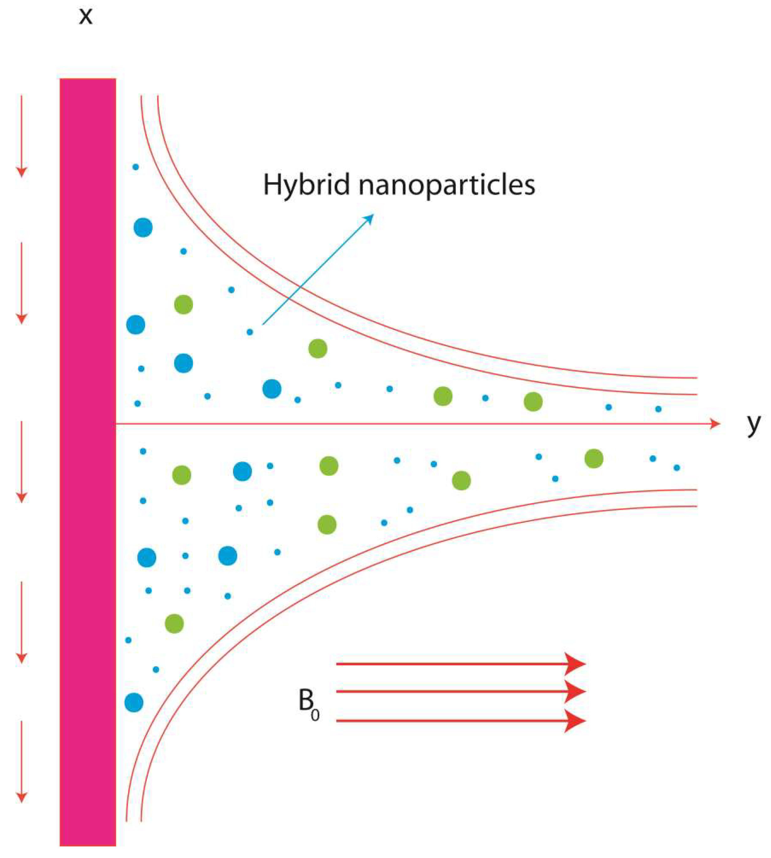
2. Physical Statement of the Problem

A phenomenon of heat and mass transfer in a Casson liquid is observed towards the vertical melting surface. A constant magnetic field is exerted along the y-axis of the surface. The fluid runs due to the stretching of the surface moving along with velocity ($u=ax$). The Nano and hybrid nanoparticles have an important role when inserted into the base fluid for simulating the enhancement of heat and solute in fluid particles. The external heat source/sink is also considered in the heat equation carrying Joule heating, viscous dissipation, and the Dufour and Soret effects. The geometry of fluid behavior is considered in Figure 1. The following assumptions are considered:

➢

A constant magnetic field is considered,

➢

Dufour and Soret effects are addressed,

➢

A porous vertical surface is considered,

➢

Casson fluid particles are inserted,

➢

A phenomenon of Joule heating is noticed,

➢

The finite element method is used,

➢

Nano and hybrid nanoparticles are observed.

The following PDEs (partial differential equations) are used utilizing BLA (boundary layer thickness):

$$\frac{\partial u}{\partial x}+\frac{\partial v}{\partial y}=0,$$

(1)

$$\begin{gathered} u\frac{\partial u}{\partial x}+v\frac{\partial u}{\partial y}=\frac{1}{{\rho }_{hnf}}\left({\mu }_{hnf}+\frac{p_y}{\sqrt{2{\pi }_c}}\right)\frac{{\partial }^{2}u}{{\partial }^{2}y}+{({\beta }_{hnf})}_{T}g\left(T-T_{\infty }\right) \\ +{({\beta }_{hnf})}_{c}g\left(C-C_{\infty }\right)-\frac{{\sigma }_{hnf}{B}_0^{2}u}{{\rho }_{hnf}}-{\mu }_{hnf}\frac{u}{K_1}, \end{gathered}$$

(2)

$$\frac{\partial T}{\partial x}+v\frac{\partial T}{\partial y}=\frac{K_{hnf}}{{\left(\rho c_p\right)}_{hnf}}\frac{{\partial }^{2}u}{{\partial }^{2}y}+\frac{1}{{\left(\rho c_p\right)}_{hnf}}\left({\mu }_{hnf}+\frac{p_y}{\sqrt{2{\pi }_c}}\right){\left(\frac{\partial u}{\partial y}\right)}^2+\frac{{\sigma }_{hnf}{B}_0^2{u}^2}{{\left(\rho c_p\right)}_{hnf}}+\frac{Q_0}{{\left(\rho c_p\right)}_{hnf}}\left(T-T_{\infty }\right)+\frac{D{K}_{T}u}{C_s{C}_p}\frac{{\partial }^{2}C}{{\partial }^{2}y},$$

(3)

$$u\frac{\partial C}{\partial x}+v\frac{\partial C}{\partial y}={(D_B)}_{hnf}\frac{{\partial }^{2}C}{{\partial }^{2}y}+\frac{D_T}{T_{\infty }}\frac{{\partial }^{2}T}{{\partial }^{2}y},$$

(4)

Equation (1) is called the 2D continuity equation for incompressible and steady flow. It is noticed that boundary layer approximations and assumptions are used in the law of conservation mass. Equation (2) is known as the momentum equation in x and y directions for steady and incompressible flow. Equation (2) is derived from momentum conservation law considering the magnetic field, Casson fluid and the Bouncy effect. Equations (3) and (4) are energy and concentration equations considering effects (heat generation, Joule heating, chemical reaction, Soret and Dufour) over a vertical surface.

Slip conditions are considered and derived using the slip theory concept. Slip theory is defined as the velocity of the fluid at the boundary that is not equal to the velocity of the boundary. The mathematical form of slip conditions near the surface of the boundary is defined as:

$$\begin{array}{c}ax=u\left(x,0\right),v\left(x,0\right)=0,-\gamma k_{hnf}\frac{\partial T}{\partial y}\left(x,0\right)=h_f(T-T\left(x,0\right),T\left(x,\infty \right)=T_{\infty }\\ -\gamma D_{hnf}\frac{\partial C}{\partial y}\left(x,0\right)=h_c\left(C-C\left(x,0\right)\right),0=u\left(x,0\right),C\left(x,\infty \right)=C_{\infty },\end{array}\},$$

(5)

Composite between hybrid nanoparticles and nanomaterials [45,46] are:

$$\frac{{\rho }_{hnf}}{{\rho }_f}=\left(1-{\phi }_2\right)\left\{\left(1-{\phi }_1\right)+\frac{{\phi }_1{\rho }_{s_1}}{{\rho }_f}\right\}+\frac{{\phi }_2{\rho }_{s_2}}{{\rho }_f},$$

(6)

$$\frac{{\left(\rho c_p\right)}_{hnf}}{{\left(\rho c_p\right)}_f}=\left(1-{\phi }_2\right)\left\{\left(1-{\phi }_1\right)+\frac{{\phi }_1{\left(\rho c_p\right)}_{s_1}}{{\left(\rho c_p\right)}_f}\right\}+\frac{{\phi }_2{\left(\rho c_p\right)}_{s_2}}{{\left(\rho c_p\right)}_f},$$

(7)

$$\frac{{\mu }_{hnf}}{{\mu }_f}=\frac{1}{{\left(1-{\phi }_1\right)}^{2.5}{\left(1-{\phi }_2\right)}^{2.5}},$$

(8)

$$\begin{gathered} \frac{{\sigma }_{hnf}}{{\sigma }_{bf}}=\frac{{\sigma }_{s_2}+\left(n-1\right){\sigma }_{bf}-\left(n-1\right){\phi }_2\left({\sigma }_{bf}-{\sigma }_{s_2}\right)}{{\sigma }_{s_2}+2{\sigma }_{bf}+{\phi }_2\left({\sigma }_{bf}-{\sigma }_{s_2}\right)}, \frac{{\sigma }_{bf}}{{\sigma }_f} \\ =\frac{{\sigma }_{s_1}+2{\sigma }_f-\left(n-1\right){\phi }_1\left({\sigma }_f-{\sigma }_{s_1}\right)}{{\sigma }_{s_1}+2{\sigma }_f+{\phi }_1\left({\sigma }_f-{\sigma }_{s_1}\right)}, \end{gathered}$$

(9)

$$\begin{gathered} \frac{k_{hnf}}{k_{bf}}=\frac{k_{s_2}+2k_{bf}-\left(n-1\right){\phi }_2\left(k_{bf}-k_{s_2}\right)}{k_{s_2}+2k_{bf}+{\phi }_2\left(k_{bf}-k_{s_2}\right)}, \frac{k_{bf}}{k} \\ =\frac{k_{s_1}+2k_f-\left(n-1\right){\phi }_1\left(k_f-k_{s_1}\right)}{k_{s_1}+2k_f+{\phi }_1\left(k_f-k_{s_1}\right)}, \end{gathered}$$

(10)

$$\frac{D_{hnf}}{D_f}=\frac{1}{\left(1-{\phi }_1\right)\left(1-{\phi }_2\right)},$$

(11)

Required transformations are:

$$\begin{gathered} u=ax{f}^{\prime }\left(\eta \right), v=-\sqrt{a{\upsilon }_f}f\left(\eta \right),\eta =\sqrt{\frac{a}{{\upsilon }_f}}y,\theta \left(\eta \right)=\frac{T-T_{\infty }}{T_w-T_{\infty }}, \\ \psi \left(\eta \right)=\sqrt{a{\upsilon }_f}xf\left(\eta \right), \varphi \left(\eta \right)=\frac{C-C_{\infty }}{C_w-C_{\infty }} \end{gathered}$$

(12)

Hence, one gets:

$$\begin{gathered} \frac{{\upsilon }_{hnf}}{{\nu }_f}\left(1+\frac{1}{\beta }\right)f^{‴}-[{\left(f^{\prime }\right)}^2-f{f}^{″}]+{\left(Gr\right)}_T\theta \left(\eta \right)+{\left(Gr\right)}_C\varphi \left(\eta \right) \\ -M\left(\frac{{\sigma }_{hnf}}{{\sigma }_f}\right)\left(\frac{{\rho }_f}{{\rho }_{hnf}}\right)f^{’}-K{f}^{\prime }=0, \\ \left(\frac{K_{hnf}}{K_f}\right)\left(\frac{{\rho }_f}{{\rho }_{hnf}}\right)\left(\frac{{(C_p)}_f}{{(C_p)}_{hnf}}\right){\theta }^{’’}+\left(\frac{{\upsilon }_{hnf}}{{\nu }_f}\right)\left(\frac{{(C_p)}_f}{{(C_p)}_{hnf}}\right)\left(1+\frac{1}{\beta }\right)PrEc{\left(f^{″}\right)}^2 \end{gathered}$$

(13)

$$+\left(\frac{{\sigma }_{hnf}}{{\sigma }_f}\right)\left(\frac{{(C_p)}_f}{{(C_p)}_{hnf}}\right)\left(\frac{{\rho }_f}{{\rho }_{hnf}}\right)MEc{\left( f^{’’}\right)}^2+fPr{\theta }^{\prime }+Pr{\beta }^{*}\theta +Pr{D}_f{\varphi }^{″}=0,$$

(14)

$${\varphi }^{″}+ScSr{\theta }^{″}+Scf{\varphi }^{\prime }= 0,$$

(15)

Associated BCs are formulated as:

$$\begin{array}{c}f\left(0\right)=0, {\theta }^{\prime }\left(0\right)=\frac{{\beta }_i}{\gamma }\left(1-\theta \left(0\right)\right), {\varphi }^{\prime }\left(0\right)=\frac{E_i}{\alpha }\left(1-\varphi \left(0\right)\right), f^{\prime }\left(0\right)=1 \\ f^{\prime }(\infty )=\theta (\infty )=\varphi (\infty )=0 . \end{array}\}$$

(16)

$$\begin{array}{c}{\left(Gr\right)}_t=\frac{g\left(T_w-T_{\infty }\right){\left({\beta }_{hnf}\right)}_T}{a^{2}x},{\left(Gr\right)}_c=\frac{g\left(C_w-C_{\infty }\right){\left({\beta }_{hnf}\right)}_C}{a^{2}x},M=\frac{{\sigma }_f{B}_0^2}{{\rho }_{f}a},K=\frac{{\mu }_f}{a{K}_1}\\ Ec=\frac{a^2{x}^2}{c_p\left(T_w-T_{\infty }\right)}, Pr=\frac{{\mu }_f{\left(c_p\right)}_f}{k_f},{\beta }^{*}=\frac{Q_0}{a{\left(\rho c_p\right)}_f},D_f=\frac{D{k}_T\left(C_w-C_{\infty }\right)}{C_s{C}_p\left(T_w-T_{\infty }\right)},\\ Sc=\frac{D_T\left(T_w-T_{\infty }\right)\left(1-{\phi }_1\right)\left(1-{\phi }_2\right)}{{\upsilon }_f{T}_{\infty }{D}_f\left(C_w-C_{\infty }\right)},Sc=\frac{{\upsilon }_f\left(1-{\phi }_1\right)\left(1-{\phi }_2\right)}{D_f} ,B_i=\frac{h_f}{k_{hnf}}\sqrt{\frac{{\upsilon }_f}{a}}.\end{array}\}$$

(17)

It is noticed that the physical magnitude reveals a dynamically mutual fluid-structure interaction at a rigid interface in which the strength of viscous frictional forces are evaluated as the trough skin friction coefficient called factor $C_f$. Surface force is also called the skin friction coefficient. The skin friction coefficient, Nusselt number and concentration gradient are:

$$\begin{array}{c}{C}_f=\frac{{\tau }_{xy|y=0}}{{\rho }_f{U}_0^2}=\frac{f^{″}\left(0\right)}{R{e}_x^{\raisebox{1ex}{$1$}\!\left/ \!\raisebox{-1ex}{$2$}\right.}{\left(1-{\phi }_1\right)}^{2.5}{\left(1-{\phi }_2\right)}^{2.5}},\\ Nu=\frac{-x{k}_{hnf}{\frac{\partial T}{\partial y}|}_{y=0}}{k_f\left(T_w-T_{\infty }\right)}=\frac{-R{e}_x^{\raisebox{1ex}{$1$}\!\left/ \!\raisebox{-1ex}{$2$}\right.}{k}_{hnf}}{k_f}{\theta }^{\prime }\left(0\right),\\ Sh=\frac{-x{D}_{hnf}{\frac{\partial C}{\partial y}|}_{y=0}}{D_f\left(C_w-C_{\infty }\right)}=\frac{-R{e}_x^{\raisebox{1ex}{$1$}\!\left/ \!\raisebox{-1ex}{$2$}\right.}}{\left(1-{\phi }_1\right)\left(1-{\phi }_2\right)}{\varphi }^{\prime }\left(0\right),\end{array}\}$$

(18)

where ${Re}_x=\frac{a{x}^2}{{\nu }_f}$ is the Reynolds number. Thermo-physical properties are shown in

Table 1. Values of properties of nano-structures and hybrid nano-structures.

Physical Property	Ethylene Glycol (EG)	MOS2	MOS2/SiO2
$\rho \left(\mathrm{K}\mathrm{g}/{\mathrm{m}}^3\right)$	1113.5	2650	5060
$k\left(\mathrm{W}/\left(\mathrm{m}·\mathrm{K}\right)\right)$	2430	730	397.746
$c_p\left(\mathrm{J}/\left(\mathrm{k}\mathrm{g}·\mathrm{K}\right)\right)$	0.253	1.5	34.5
$\sigma /\left(\Omega /\mathrm{m}\right)$	$4.3\times {10}^{-5}$	0.0005	$1\times {10}^{-18}$

. Moreover, $\tau$ is shear stress (force per unit area) applied perpendicular to the surface of the sheet.

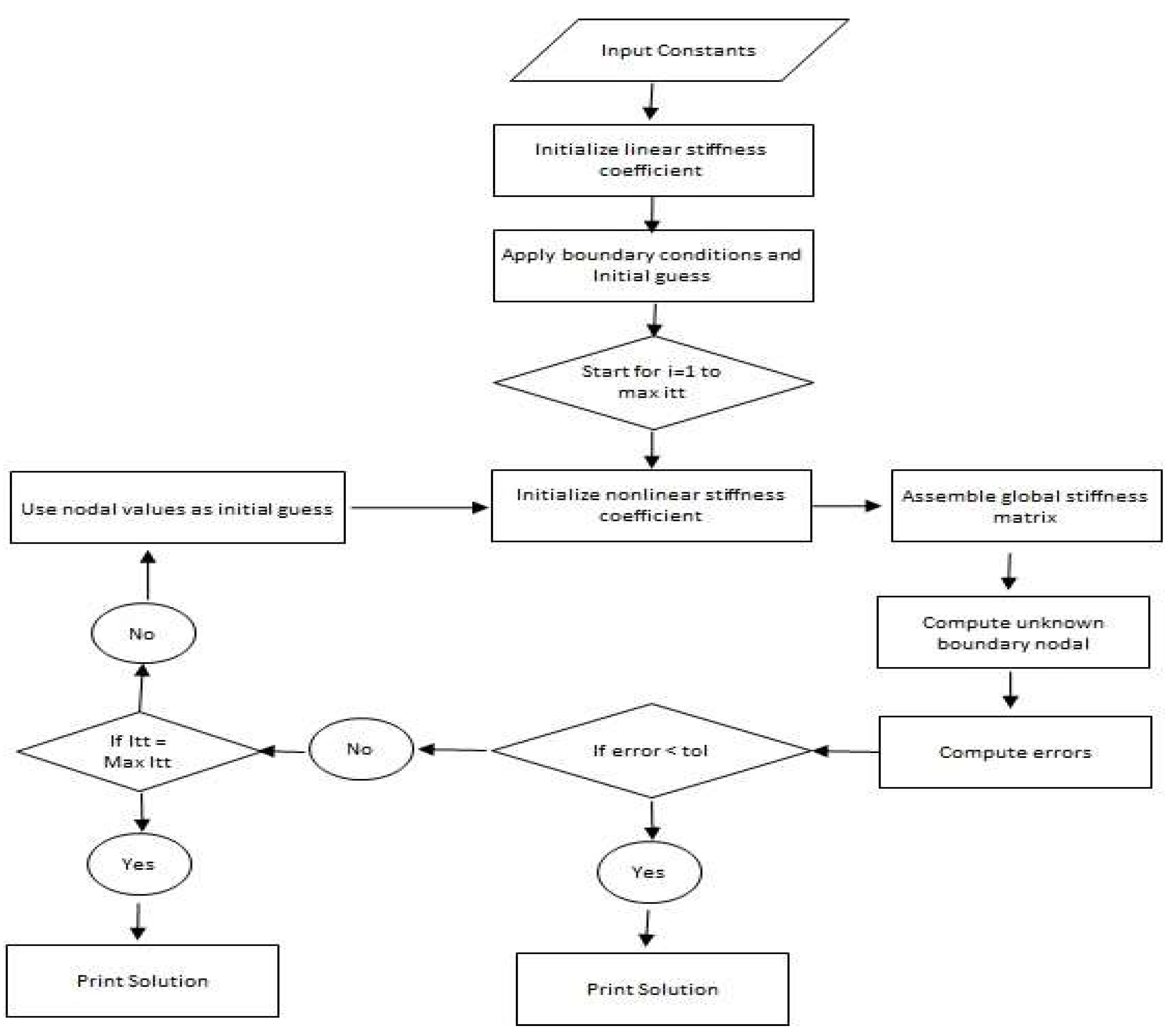
3. Numerical Procedure

The concept of the FEM is generated by structure mechanics. The vital role of the FEM is to handle complex geometries, unstructured grids and curved cells. An important phenomenon of the FEM is the discretization of the domain into elements. The FEM is a strong approach in terms of convergence, accuracy and stability rather than other numerical methods. Detailed discussion of the Galerkin finite element method can be found in [10,44,45].

The discretization of the problem domain into finite elements: Firstly, the domain of the current model is divided into the finite number of elements and a polynomial kind of solution is assumed over each element. Such approximation is then applied in the weak form (with the weighted residual scheme) which is derived from the strong form (Equations (13)–(16)). Therefore, the shape functions are multiplied with the residuals and integrated over the whole domain. The residuals of the current model are:

$${{\displaystyle \int }}_{{\eta }_e}^{{\eta }_{e+1}}{W}_1\left[f^{\prime }-S\right]d\eta =0,$$

(19)

$${{\displaystyle \int }}_{{\eta }_e}^{{\eta }_{e+1}}{W}_2\left[\begin{array}{c}\frac{{\upsilon }_{hnf}}{{\nu }_f}\left(1+\frac{1}{\beta }\right)S’’-[{\left(S\right)}^2-fS’]+{\left(Gr\right)}_T\theta \left(\eta \right)+{\left(Gr\right)}_C\varphi \left(\eta \right)\\ -M\left(\frac{{\sigma }_{hnf}}{{\sigma }_f}\right)\left(\frac{{\rho }_f}{{\rho }_{hnf}}\right)S-KS\end{array}\right]d\eta =0,$$

(20)

$${{\displaystyle \int }}_{{\eta }_e}^{{\eta }_{e+1}}{W}_3[\begin{array}{c}\left(\frac{K_{hnf}}{K_f}\right)\left(\frac{{\rho }_f}{{\rho }_{hnf}}\right)\left(\frac{{(C_p)}_f}{{(C_p)}_{hnf}}\right)\theta \text{'}\text{'}+Pr{\beta }^{*}\theta \\ +\left(\frac{{\sigma }_{hnf}}{{\sigma }_f}\right)\left(\frac{{(C_p)}_f}{{(C_p)}_{hnf}}\right)\left(\frac{{\rho }_f}{{\rho }_{hnf}}\right)MEc{\left(S\text{'}\right)}^2+fPr\theta \text{'}\\ Pr{D}_f\varphi \text{'}\text{'}+\left(\frac{{\upsilon }_{hnf}}{{\nu }_f}\right)\left(\frac{{(C_p)}_f}{{(C_p)}_{hnf}}\right)\left(1+\frac{1}{\beta }\right)PrEc{\left(S\text{'}\right)}^2\end{array}]d\eta =0,$$

(21)

$${{\displaystyle \int }}_{{\eta }_e}^{{\eta }_{e+1}}{W}_4\left[\varphi ’’+ScSr{\theta }^{″}+\frac{Sc}{{\left(1-{\phi }_2\right)}^{2.5}{\left(1-{\phi }_1\right)}^{2.5}}f\varphi ’\right]d\eta =0,$$

(22)

where $W_1, W_2, W_3$ and $W_4$ are called the shape functions, $f’$ is considered as $S$ for the Galerkin approach. Shape functions and variables used in the problem are:

$${\chi }_j={\left(-1\right)}^{l-1}\frac{1-\frac{\eta }{{\eta }_{l-1}}}{1-\frac{{\eta }_l}{{\eta }_{l-1}}},$$

(23)

where $l$ is considered as 1 and 2, respectively:

$$f={\displaystyle \sum }_{l=1}^2\left(f_l{\chi }_j\right), F={\displaystyle \sum }_{l=1}^2\left(F_l{\chi }_j\right),$$

(24)

$$\theta ={\displaystyle \sum }_{l=1}^2\left({\theta }_l{\chi }_j\right), \varphi ={\displaystyle \sum }_{l=1}^2\left({\varphi }_l{\chi }_j\right).$$

(25)

Problem domain: The computational domain is made with the help of the problem domain while the problem domain is considered $\left[0, \infty \right)$. It is observed that asymptotic BCs are satisfied by assuming ${\eta }_{\infty }=6$. Therefore, in this current model, the computation domain is $\left[0, 6\right]$.

Assembly process: This procedure plays a vital role to obtain the stiffness matrix, force vector, and integral boundary vector over the whole domain of the problem. Finally, the global stiffness matrix is simulated with the help of the assembly process. The Galerkin approach is used to find the stiffness elements that are:

$$K_{ij}^{11}={{\displaystyle \int }}_{{\eta }_e}^{{\eta }_{e+1}}{\chi }_i\left(\frac{d{\chi }_j}{d\eta }\right)d\eta ,K_{ij}^{12}=-{{\displaystyle \int }}_{{\eta }_e}^{{\eta }_{e+1}}{\chi }_i\left({\chi }_j\right)d\eta ,$$

(26)

$$K_{ij}^{13}=0, K_{ij}^{14}=0,K_{ij}^{21}=0,K_{ij}^{42}=0,$$

(27)

$$K_{ij}^{23}={{\displaystyle \int }}_{{\eta }_e}^{{\eta }_{e+1}}{\left(Gr\right)}_T{\chi }_i\left({\chi }_j\right)d\eta ,B_i^1=0,B_i^4=0,$$

(28)

$$K_{ij}^{24}={{\displaystyle \int }}_{{\eta }_e}^{{\eta }_{e+1}}{\left(Gr\right)}_C{\chi }_i\left({\chi }_j\right)d\eta ,B_i^2=0,B_i^3=0,$$

(29)

$$K_{ij}^{33}={{\displaystyle \int }}_{{\eta }_e}^{{\eta }_{e+1}}\left[\begin{array}{c}-\left(\frac{K_{hnf}}{K_f}\right)\left(\frac{{\rho }_f}{{\rho }_{hnf}}\right)\left(\frac{{(C_p)}_f}{{(C_p)}_{hnf}}\right)\frac{d{\chi }_j}{d\eta }\frac{d{\chi }_i}{d\eta }+\\ Pr{\beta }^{*}{\chi }_i\left({\chi }_j\right)+\overline{F}Pr{\chi }_i\frac{d{\chi }_j}{d\eta }\end{array}\right]d\eta ,$$

(30)

$$K_{ij}^{22}={{\displaystyle \int }}_{{\eta }_e}^{{\eta }_{e+1}}\left[\begin{array}{c}-\frac{{\nu }_{hnf}}{{\nu }_f}\left(1+\frac{1}{\beta }\right)\frac{d{\chi }_j}{d\eta }\frac{d{\chi }_i}{d\eta }-\overline{S}{\chi }_i\frac{d{\chi }_j}{d\eta }-\overline{f}{\chi }_i\frac{d{\chi }_j}{d\eta }]\\ -M\left(\frac{{\sigma }_{hnf}}{{\sigma }_f}\right)\left(\frac{{\rho }_f}{{\rho }_{hnf}}\right){\chi }_i\left({\chi }_j\right)-K{\chi }_i\left({\chi }_j\right)\end{array}\right]d\eta ,$$

(31)

$$K_{ij}^{31}={{\displaystyle \int }}_{{\eta }_e}^{{\eta }_{e+1}}\left[\begin{array}{c}\left(\frac{{\upsilon }_{hnf}}{{\nu }_f}\right)\left(\frac{{(C_p)}_f}{{(C_p)}_{hnf}}\right)\left(1+\frac{1}{\beta }\right)PrEc\overline{S^{\prime }}{\chi }_i\frac{d{\chi }_j}{d\eta }\\ \left(\frac{{\sigma }_{hnf}}{{\sigma }_f}\right)\left(\frac{{(C_p)}_f}{{(C_p)}_{hnf}}\right)\left(\frac{{\rho }_f}{{\rho }_{hnf}}\right)MEc\overline{S^{\prime }}{\chi }_i\frac{d{\chi }_j}{d\eta }\end{array}\right]d\eta ,$$

(32)

$$K_{ij}^{34}={{\displaystyle \int }}_{{\eta }_e}^{{\eta }_{e+1}}\left[-Pr{D}_f\frac{d{\chi }_j}{d\eta }\frac{d{\chi }_i}{d\eta }\right]d\eta ,K_{ij}^{32}=0,K_{ij}^{34}=0,$$

(33)

$$K_{ij}^{43}=-{{\displaystyle \int }}_{{\eta }_e}^{{\eta }_{e+1}}\left(\frac{d{\chi }_j}{d\eta }\frac{d{\chi }_i}{d\eta }\right)d\eta ,K_{ij}^{51}=0,K_{ij}^{41}=0,$$

(34)

$$K_{ij}^{43}=-{{\displaystyle \int }}_{{\eta }_e}^{{\eta }_{e+1}}\left[-\frac{d{\chi }_j}{d\eta }\frac{d{\chi }_i}{d\eta }+\frac{\overline{f}{\chi }_i\frac{d{\chi }_j}{d\eta }Sc}{{\left(1-{\phi }_2\right)}^{2.5}{\left(1-{\phi }_1\right)}^{2.5}}\right]d\eta ,$$

(35)

Picard linearization approach: This approach is used to convert non-linear equations to linear equations. This approach is called the linearization approach. In the current model, the Picard linearization approach is utilized to obtain the linear system of equations:

$$\overline{S}={\displaystyle \sum }_{j=1}^2{\chi }_j\overline{S_j}, \overline{f}={\displaystyle \sum }_{j=1}^2{\chi }_j\overline{f_j}.$$

(36)

Here $\overline{S_j}$ and $\overline{f_j}$ are nodal (unknown) values. The flow chart of this Picard linearisation approach is captured in Figure 2.

The Picard approach is used to simulate the heat conduction problems related to the local fractional. This approach is also used to determine the non-differential solution of the heat equation in view of the fractal media and non-differential solution. One of the most vital advantages is that it converts highly non-linear equations into linear equations. The engineering and heat transfer problems are associated with PDEs (partial differential equations). The Picard approach is used to simulate such equations in terms of the engineering and industrial fields.

Error analysis: The error analysis is simulated by the following equation that is:

$$Error=\left|{\tau }^j-{\tau }^{j-1}\right|,$$

(37)

and convergence criteria is mentioned as:

$$Max\left|{\tau }^j-{\tau }^{j-1}\right|<{10}^{-5}.$$

(38)

Meshfree analysis: In this analysis, convergence analysis is tested in terms of a grid-independent study. This analysis is carried out in

Table 2. Mesh-free analysis of $f’\left(\frac{{\eta }_{max}}{2}\right), \theta \left(\frac{{\eta }_{max}}{2}\right)$ and $\varphi \left(\frac{{\eta }_{max}}{2}\right)$ at the mid of the computational domain $\left[0, 6\right]$.

Number of Elements	$\mathit{f}’\left(\frac{{\mathit{\eta }}_{\mathit{m}\mathit{a}\mathit{x}}}{2}\right)$	$\mathit{\theta }\left(\frac{{\mathit{\eta }}_{\mathit{m}\mathit{a}\mathit{x}}}{2}\right)$	$\mathit{\varphi }\left(\frac{{\mathit{\eta }}_{\mathit{m}\mathit{a}\mathit{x}}}{2}\right)$
30	0.008089866763	0.01503704758	0.02481424434
60	0.008692521344	0.008731223985	0.01864316747
90	0.008867852479	0.006377768777	0.01586843723
120	0.008952109139	0.005111048492	0.01419676870
150	0.009001959002	0.004307605387	0.01304491414
180	0.009034938370	0.003747398644	0.01218677926
210	0.009058498510	0.003331898105	0.01151399434
240	0.009076411866	0.003009949525	0.01096716142
270	0.009034320136	0.003009949525	0.01096716142
300	0.009094305031	0.003010348213	0.01092535030

. The simulations are recorded at the mid of each element. The solution converges after the simulations of 300 elements. Hence, 300 elements are required for convergence of the problem. The mesh-free analysis is known as a grid-independent study. The outcomes are recorded of $f^{’\left(\frac{{\eta }_{max}}{2}\right)}, \theta \left(\frac{{\eta }_{max}}{2}\right)$ and $\varphi \left(\frac{{\eta }_{max}}{2}\right)$ at the mid of each 300 elements. Hence, the solution of the problem is converged at 300 elements.

Table 3. Comparative study of a temperature gradient with published results of Qureshi et al. [45] in the case of nanofluid.

	[45]	present results
	Nusselt number	Nusselt number
	0.68	0.681052103137
$k_{nf}$	0.72141	0.723331807103
	0.82458	0.824720819103

reveals the comparative results of the Nusselt number with published work [40].

Comparative study: It is observed that the results of the present problem are simulated with the help of the finite element method. Table 3 reveals a validation of results in view of the Nusselt number for the case of nanofluid. In Table 3, published results [47] are simulated by a shooting approach whereas these results are verified with the finite element method.

Table 4. Comparative numerical values of Nusselt number with shooting method for nanofluid.

	Shooting Method [47]	Finite Element Method
	$Nu$	$Nu$
	0.9391	0.93890213031
$k_{nf}$	1.06696	1.06691013039

. Shows the comparative study of FEM and shooting method.

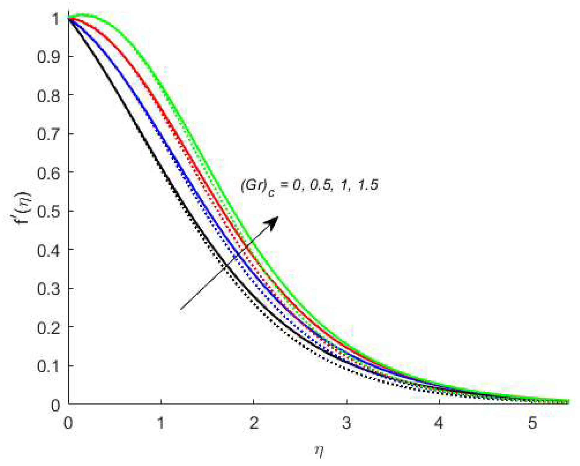
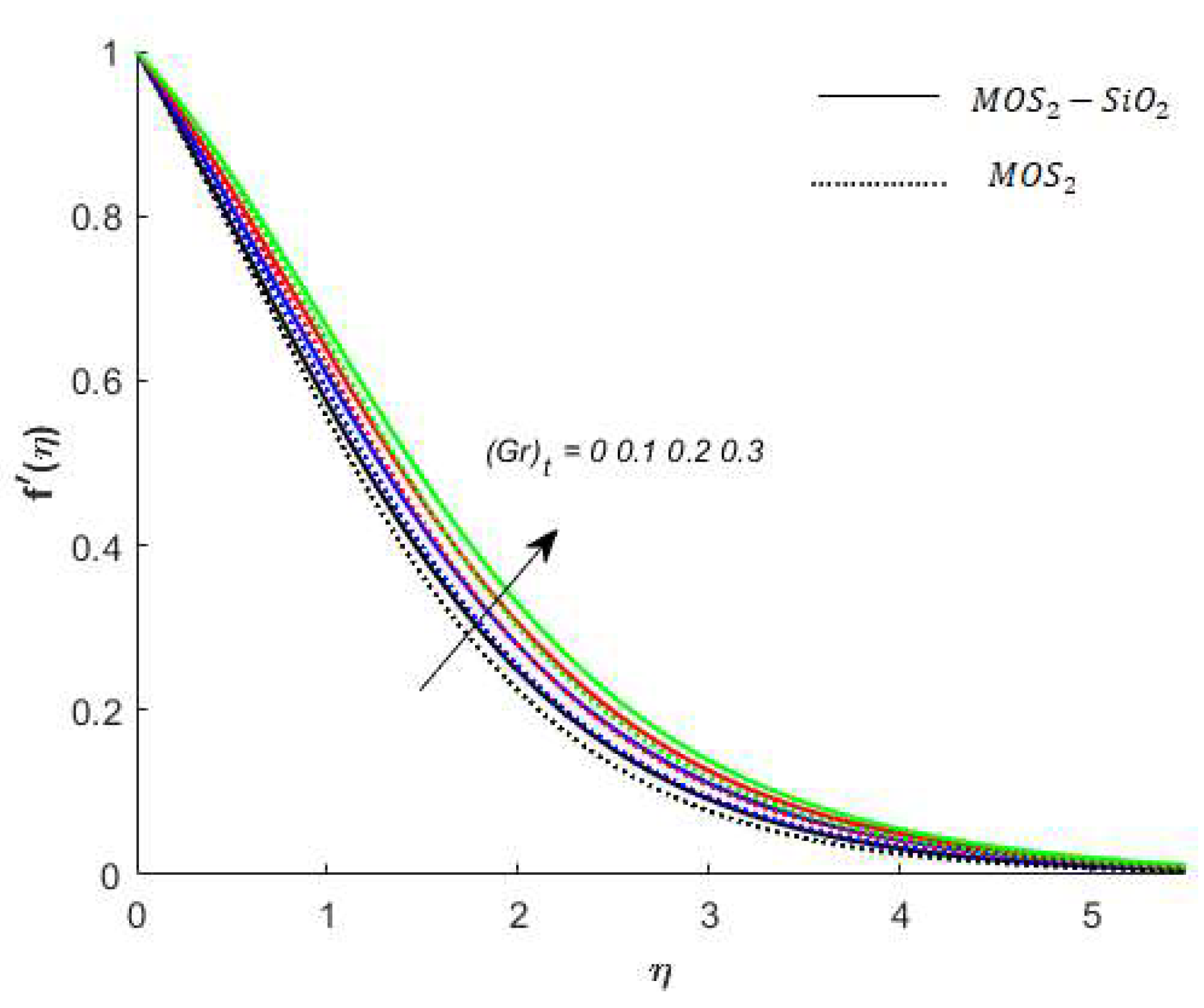
4. Outcomes and Discussion

Flow analysis: The effects of pertinent physical parameters are displayed in Figure 3, Figure 4, Figure 5, Figure 6, Figure 7, Figure 8, Figure 9, Figure 10, Figure 11, Figure 12, Figure 13, Figure 14, Figure 15 and Figure 16. This parameter is defined as the ratio between the viscous force and buoyancy force.

Variation in the velocity of nanofluids under the influences of ${\left(Gr\right)}_c$ is presented in Figure 3. Figure 3 reveals that the velocity of the nanofluids is an increasing function of ${\left(Gr\right)}_c$ and the reason for this is that when ${\left(Gr\right)}_c$ increases, it loosens up the intermolecular forces within the nanofluids and thereby enhances the velocity of the nanofluids. Figure 4 displays the behavior of ${\left(Gr\right)}_t$ on the nanofluids’ temperature. It is observed in Figure 4 that the temperature of the nanofluids’ has a direct relation with ${\left(Gr\right)}_t$, which is due to an enhancement in the nanofluids’ volumetric expansion. The effect of $K$ on the velocity of nanofluids is displayed in Figure 5. Figure 5 reports that the velocity of the nanofluids is a decreasing function of $K$. Physically, $K$ enhances the resistance to nanofluids causing a reduced velocity of the nanofluids. Figure 6 demonstrates the impact of $\beta$ (this parameter appears due to using a Casson liquid in the flow analysis) on the velocity profile of the nanofluids. It is observed in Figure 6 that the velocity of the nanofluids is a decreasing function of $\beta$. Physically, when $\beta$ is added to the nanofluids, the friction between particles slows. An inverse proportional relation is addressed among the Casson number and the motion of fluid particles. In Figure 1, Figure 2, Figure 3 and Figure 4, it is noted that the velocity profiles of the hybrid nanofluid ($MO{S}_2-Si{O}_2$) is higher than the nanofluid ($MO{S}_2$). Figure 5 and Figure 6 elucidate the impacts of the magnetic field (the magnetic field is called the vector field near the region of the electric field in forces related to where the magnetic field is observed) on the velocity and temperature of nanofluids. It is noted in Figure 5 and Figure 6 that velocity is enhanced with an increase in the magnetic field, while an opposite trend is found in the temperature profile. Physically, the Lorentz force produced due to the magnetic field is in the same direction of the nanofluids’ motion, so the flow boundary layer thickness increases and the thermal boundary layer decreases. Figure 5 also shows that the velocity of the nanofluid ($MO{S}_2$) is higher when compared to the hybrid nanofluid ($MO{S}_2-Si{O}_2$), while an opposite trend is noted in the temperature profile (Figure 6).

Temperature analysis: Figure 7 demonstrates the effect of $Ec$ (this parameter expresses ration among the enthalpy difference and the flow’s kinetic energy) on the temperature of nanofluids. It is observed from Figure 7, that $Ec$ has an inverse relation with the temperature profile. The reason for this is that the heat transfer rate at the surface increases, thus, the thermal boundary layer thickness decreases with increases in the numerical value of $Ec$. Figure 8 depicts the impact of $\beta$ on the temperature of nanofluids. The temperature of nanofluids decreases with the increase of $\beta$. The external heat source has an important impact on the temperature gradient of nanofluids, resulting in a decrement in both the thermal state of the nanofluid and temperature distribution. The variation effect of Bi on the nanofluids’ temperature is plotted in Figure 9. Figure 9 shows that the temperature of the nanofluids’ increases with an increase in the Bi. Physically, the temperature gradient near the surface increases when increasing the numerical values of Bi and hence the thickness of the thermal boundary layer increases. Figure 10 reveals the variation in temperature with the effect of $Pr$ (fractional between momentum to thermal boundary layers). It is noted from Figure 10 that the temperature of the nanofluids’ decreases as the numerical value of $Pr$ is increased. This occurred because the thermal conductivity of the nanofluids’ decreased with an increase in the $Pr$. Figure 7, Figure 8, Figure 9 and Figure 10 report that the temperature profile is greater in the case of the hybrid nanofluid ($MO{S}_2-Si{O}_2$). The impact of $Sr$ on the concentration profile is depicted in Figure 11. It is observed from Figure 11 that $Sr$ has a direct relation with the concentration profile. The reason for this is that the $Sr$ impact refers to the mass flux from a lower to greater solute concentration produced by the temperature gradient. The variation in the concentration profile under the influences of $Sc$ is presented in Figure 12. It is observed in Figure 12 that the concentration profile decreased with an increased numerical value of $Sc$ (ratio between mass diffusivity and momentum diffusivity). Physically, the kinematic viscosity increases with an increase in the $Sc$ which turns the molecular diffusion, therefore, the velocity of the nanofluids’ decreases.

Concentration analysis: Figure 13 shows that the concentration profile increases versus the higher values of $Sr.$ Figure 14 reveals a decreasing trend into solute particles when $Sc$ is increased. The role of $Ei$ versus concentration is observed in Figure 15 while the concentration increases. The reason for this is that as $Ei$ increases, mass diffusivity decreases and as a result of the concentration of nanofluids increases. Figure 16 reveals the variation of the concentration profile under the influences of $\alpha$. It is noted from Figure 16 that the concentration profile has an inverse relation with $\alpha$.

Analysis of the Sherwood, skin friction coefficient and Nusselt number: 

Table 5. Local skin friction coefficient, Nusselt number and Sherwood number for hybrid nanofluid ($MO{S}_2-Si{O}_2$) and nanofluid ($MO{S}_2$) when $M=0.2, Pr=2.36, Sr=0.1, Sc=0.8, {\left(Gr\right)}_c=0.1, K=0.1, \mathrm{and} {\beta }^{*}=0.1$.

		$\mathbf{Hybrid}\mathbf{Nanofluid}(\mathit{M}\mathit{O}{\mathit{S}}_2-\mathit{S}\mathit{i}{\mathit{O}}_2)$			$\mathbf{Nanofluid}\left(\mathit{M}\mathit{O}{\mathit{S}}_2\right)$
		$\mathit{R}{\mathit{e}}^{\frac{1}{2}}{\mathit{C}}_{\mathit{f}}$	$\mathit{R}{\mathit{e}}^{-\frac{1}{2}}\mathit{N}\mathit{u}$	$\mathit{R}{\mathit{e}}^{-\frac{1}{2}}\mathit{S}\mathit{h}$	$\mathit{R}{\mathit{e}}^{\frac{1}{2}}{\mathit{C}}_{\mathit{f}}$	$\mathit{R}{\mathit{e}}^{-\frac{1}{2}}\mathit{N}\mathit{u}$	$\mathit{R}{\mathit{e}}^{-\frac{1}{2}}\mathit{S}\mathit{h}$
	0.2	0.797275	0.584809	0.471631	0.366215	0.515542	0.392980
$E_i$	0.3	0.781452	0.582914	0.553971	0.361498	0.513625	0.437901
	0.4	0.775078	0.582143	0.587303	0.358824	0.512534	0.463449
	0.6	0.813044	0.696015	0.702877	0.359494	0.612130	0.591962
	0.4	0.831321	0.565637	0.360010	0.747694	0.623337	0.346218
$B_i$	0.5	0.829379	0.782424	0.382862	0.737070	0.645848	0.344631
	0.6	0.810632	0.602874	0.357482	0.729593	0.661806	0.343501
	0.8	0.799329	0.623448	0.356074	0.746463	0.832262	0.372349
	0.0	1.097611	0.564346	0.350003	0.995086	0.618957	0.336153
${\left(Gr\right)}_t$	0.1	0.954371	0.576780	0.354613	0.862183	0.633571	0.340746
	0.2	0.819197	0.587380	0.358536	0.737070	0.645848	0.344631
	0.3	0.690322	0.596671	0.361961	0.617928	0.656470	0.348014

presents the surface force, Nusselt number and rate of mass diffusion for ($MO{S}_2-Si{O}_2$) and nanofluid ($MO{S}_2$). The following remarks have been noted from Table 5. Under the effect of $E_i$ The local skin friction coefficient, Nusselt number and Sherwood number is higher in the case of the hybrid nanofluid ($MO{S}_2-Si{O}_2$). Surface force is more significant in the case of the hybrid nanofluid ($MO{S}_2-Si{O}_2)$ with the effect of $B_i$ and ${\left(Gr\right)}_t$. Under the effects of $B_i$ and ${\left(Gr\right)}_t$, the rate of heat transfer is higher in the nanofluid ($MO{S}_2$) as compared to the hybrid nanofluid ($MO{S}_2-Si{O}_2$).

5. Key Points of the Problem

The presented model, related to thermo-physical correlations, is developed for selected characteristics of heat and mass diffusions under the influence of viscous and Joule heating, and temperature and concentration gradients. The theoretical concepts are implemented utilizing the finite element method, with a comprehensive parametric study also presented. The following outcomes are crucial:

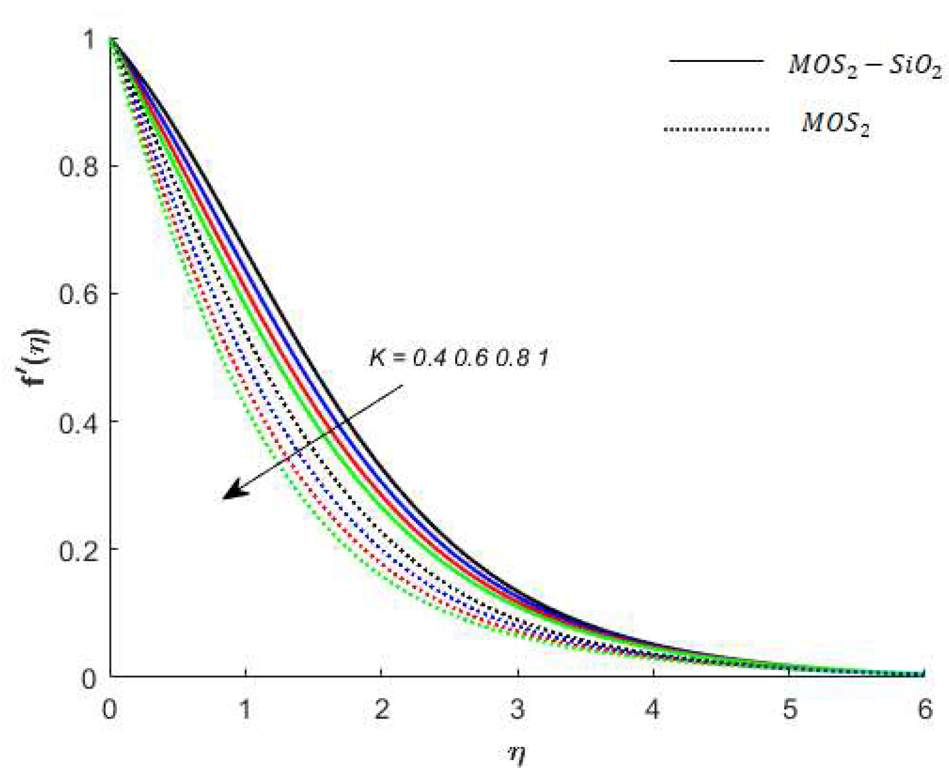
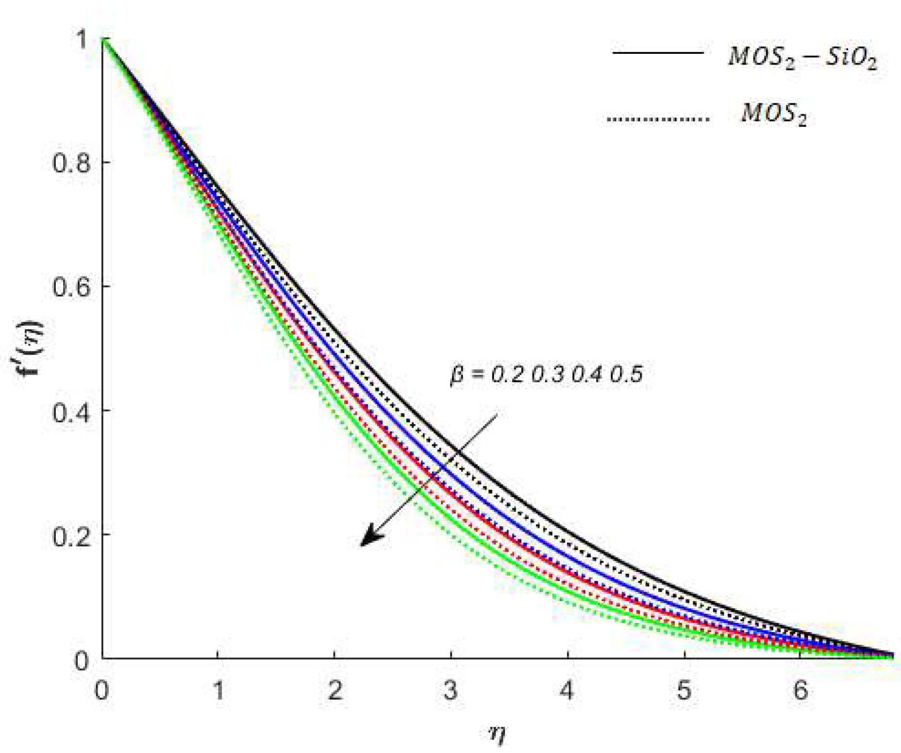
• Momentum boundary thickness is decreased against a variation in a magnetic field.
• The adjusting of BLT is controlled by varying the magnitude of the magnetic number.
• The fluid magnetic field interactions with hybrid nanofluid particles are more significant than the magnetic fluid interaction in the case of the nanofluid. Therefore, Joule heating in the hybrid nanofluid is more significant than that in the nanofluid.
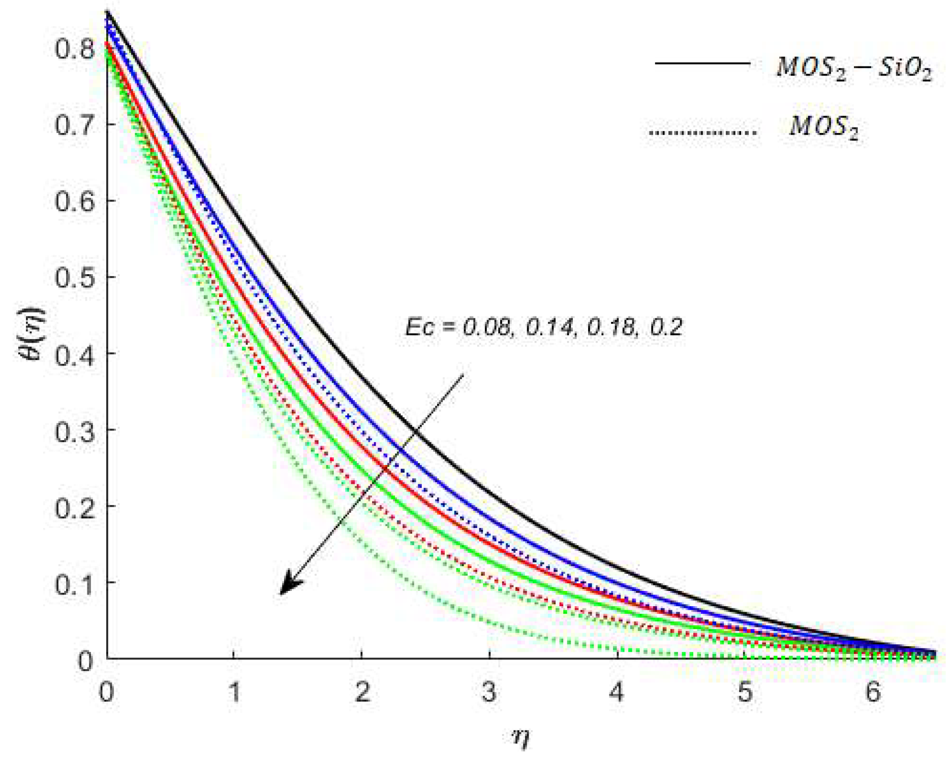
• The role of dissipation of the thermal energy and heat generation is helpful for an enhancement in thermal performance. Further, BLT is inclined versus the variation of dissipation of thermal energy and heat generation.
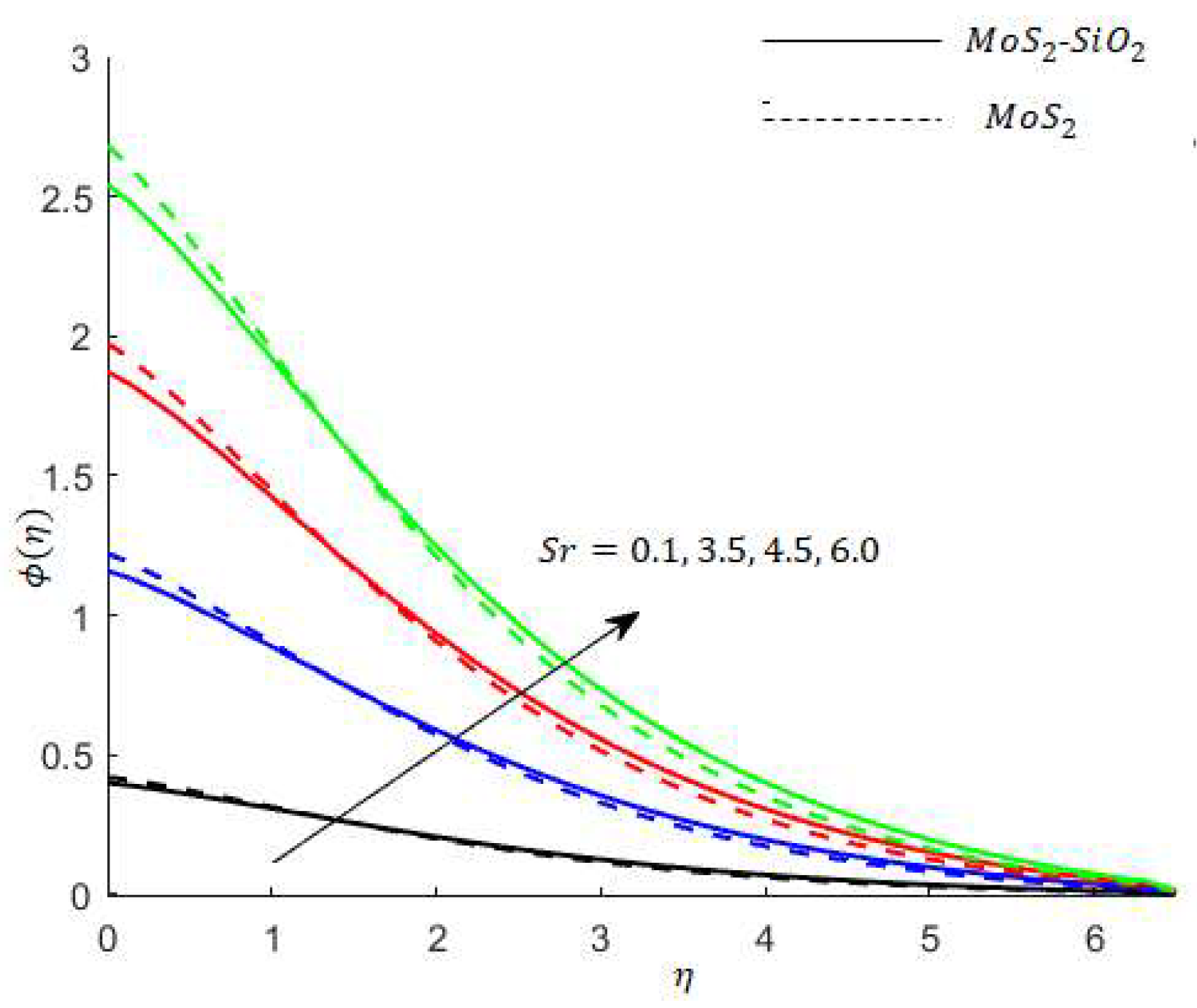
• The rate of solute particles is inclined versus enhancement in the Soret number.
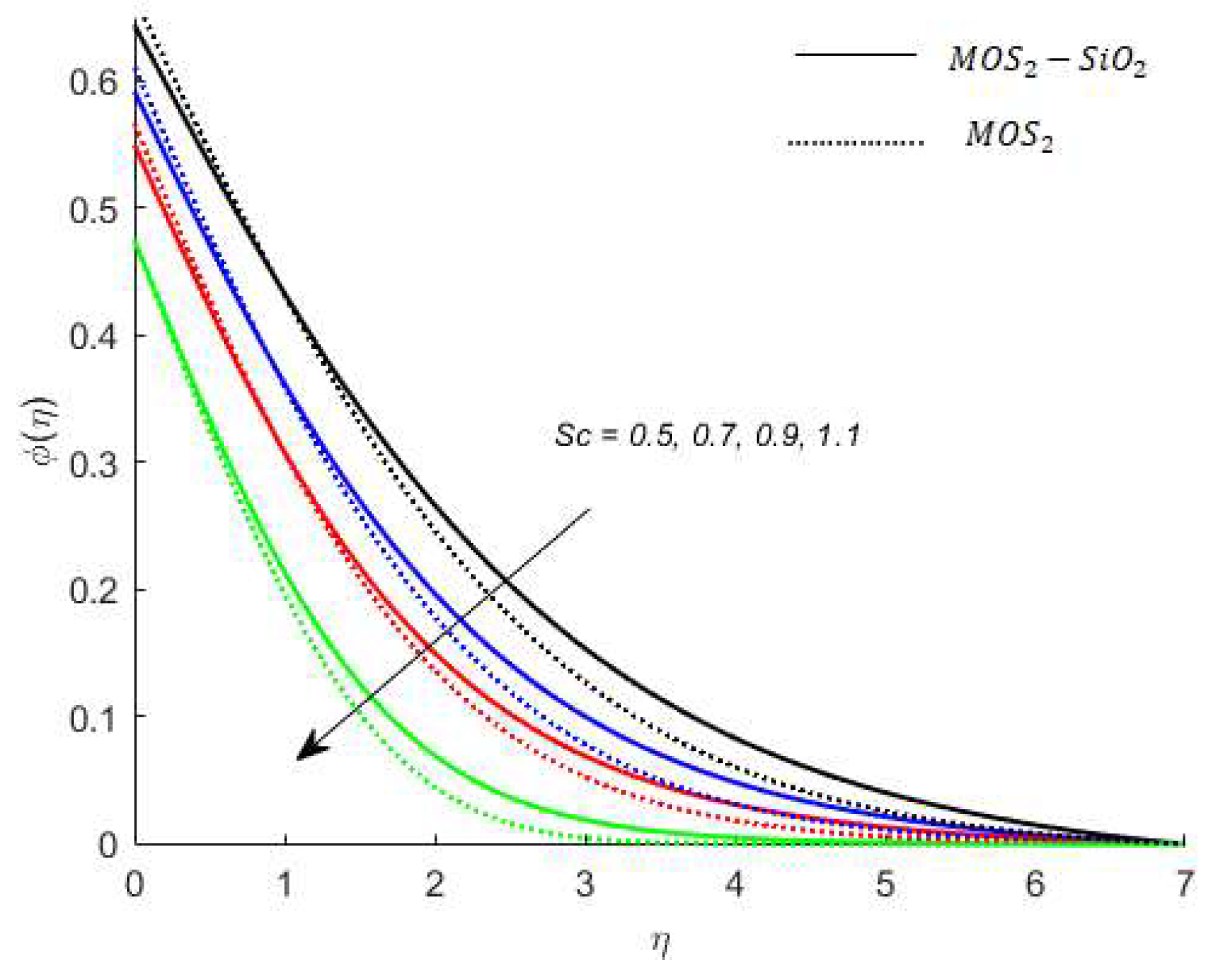
• In the porous medium, drag force exists due to the flow end; hence the convective transfer of heat and mass is compromised.
• Maximum production of heat energy is achieved for the case of hybrid nanoparticles rather than the production of heat energy for nanoparticles.
• Maximum acceleration is produced in the motion of particles for hybrid nanoparticles rather than the case of nanoparticles.
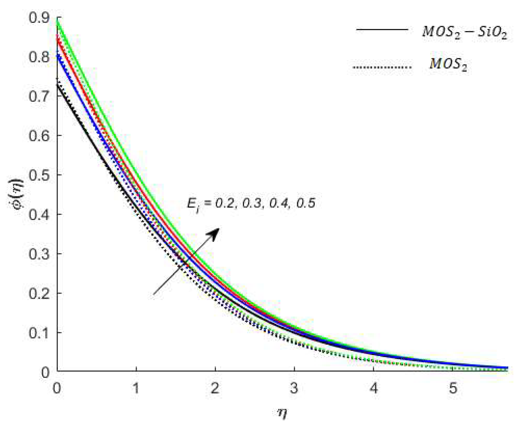
• Temperature and concentration gradients are significantly boosted for hybrid nanoparticles rather than nanoparticles.
• Convergence of the problem is obtained for 300 elements.

References

1. Masuda, H.; Ebata, A.; Teramae, K. Alteration of thermal conductivity and viscosity of liquid by dispersing ultra-fine particles. Dispersion of Al2O3, SiO2 and TiO2 ultra-fine particles. Netuse Bussei 1993, 7, 227–233. [Google Scholar] [CrossRef]
2. Choi, S.U.; Eastman, J.A. Enhancing Thermal Conductivity of Fluids with Nanoparticles; Argonne National Lab: Lemont, IL, USA, 1995. [Google Scholar]
3. Phelan, P.E.; Bhattacharya, P.; Prasher, R.S. Nanofluids for heat transfer applications. Annu. Rev. Heat Transf. 2005, 14, 255–275. [Google Scholar] [CrossRef]
4. Lee, S.; Choi, S.U.-S.; Li, S.; Eastman, J. Measuring thermal conductivity of fluids containing oxide nanoparticles. J. Heat Transf. 1999, 121, 280–289. [Google Scholar] [CrossRef]
5. Eastman, J.A.; Jeffery, A.; Choi, S.U.; Shaoping, L.; Thompson, L.J.; Lee, S. Enhanced thermal conductivity through the development of nanofluids. MRS Online Proc. Libr. Arch. 1996, 457, 220–236. [Google Scholar] [CrossRef] [Green Version]
6. Huaqing, X.; Wang, J.; Tonggeng, X.; Liu, Y.; Wu, Q. Thermal conductivity enhancement of suspensions containing nano-sized alumina particles. J. Appl. Phys. 2002, 91, 4568–4572. [Google Scholar]
7. Yimin, X.; Li, Q. Heat transfer enhancement of nanofluids. Int. J. Heat Fluid Flow 2000, 21, 58–64. [Google Scholar]
8. Keblinski, P.; Phillpot, S.; Choi, S.; Eastman, J. Mechanisms of heat flow in suspensions of nano-sized particles (nanofluids). Int. J. Heat Mass Transfer. 2002, 45, 855–863. [Google Scholar] [CrossRef]
9. Naseem, T.; Nazir, U.; Sohail, M.; Alrabaiah, H.; Sherif, E.-S.M.; Park, C. Numerical exploration of thermal transport in water-based nanoparticles: A computational strategy. Case Stud. Therm. Eng. 2021, 45, 101334. [Google Scholar] [CrossRef]
10. Nazir, U.; Nawaz, M.; Alharbi, S.O. Thermal performance of magnetohydrodynamic complex fluid using nano and hybrid nanoparticles. Phys. A Stat. Mech. Its Appl. 2020, 553, 124345. [Google Scholar] [CrossRef]
11. Koriko, O.K.; Shah, N.A.; Saleem, S.; Chung, J.D.; Omowaye, A.J.; Oreyeni, T. Exploration of bioconvection flow of MHD thixotropic nanofluid past a vertical surface coexisting with both nanoparticles and gyrotactic microorganisms. Sci. Rep. 2021, 11, 16627. [Google Scholar] [CrossRef]
12. Ali, A.; Saleem, S.; Mumraiz, S.; Saleem, A.; Awais, M.; Marwat, D.N.K. Investigation on TiO2—Cu/H2O hybrid nanofluid with slip conditions in MHD peristaltic flow of Jeffrey material. J. Therm. Anal. Calorim. 2021, 143, 1985–1996. [Google Scholar] [CrossRef]
13. Tian, M.-W.; Rostami, S.; Aghakhani, S.; Goldanlou, A.S.; Qi, C. A techno-economic investigation of 2D and 3D configurations of fins and their effects on heat sink efficiency of MHD hybrid nanofluid with slip and non-slip flow. Int. J. Mech. Sci. 2021, 189, 105975. [Google Scholar] [CrossRef]
14. Mumraiz, S.; Ali, A.; Awais, M.; Shutaywi, M.; Shah, Z. Entropy generation in electrical magnetohydrodynamic flow of Al2O3—Cu/H2O hybrid nanofluid with non-uniform heat flux. J. Therm. Anal. Calorim. 2021, 143, 2135–2148. [Google Scholar] [CrossRef]
15. Awais, M.; Ullah, N.; Ahmad, J.; Sikandar, F.; Ehsan, M.M.; Salehin, S.; Bhuiyan, A.A. Heat transfer and pressure drop performance of Nanofluid: A state-of-the-art review. Int. J. 2021, 9, 100065. [Google Scholar]
16. Nazir, U.; Sohail, M.; Selim, M.M.; Alrabaiah, H.; Kumam, P. Finite element simulations of hybrid nano-Carreau Yasuda fluid with hall and ion slip forces over rotating heated porous cone. Sci. Rep. 2021, 11, 19604. [Google Scholar] [CrossRef]
17. Manoj, C.; Kumar, S.; Bhandari, D.R.; Das, K.P.; Mann, I. Development and characterisation of Al2Cu and Al2Al nanoparticle dispersed water and ethylene glycol based nanofluid. Mat. Sci. Eng. 2007, 4, 141–148. [Google Scholar]
18. Ijaz, M.; Ayub, M.; Malik, M.Y.; Khan, H.; A Alderremy, A.; Aly, S. Entropy analysis in nonlinearly convective flow of the Sisko model in the presence of Joule heating and activation energy: The Buongiorno model. Phys. Scr. 2020, 95, 025402. [Google Scholar] [CrossRef]
19. Majeed, A.H.; Bilal, S.; Mahmood, R.; Malik, M.Y. Heat transfer analysis of viscous fluid flow between two coaxially rotated disks embedded in permeable media by capitalising non-Fourier heat flux model. Phys. A Stat. Mech. Its Appl. 2020, 540, 123182. [Google Scholar] [CrossRef]
20. Ali, U.; Rehman, K.U.; Malik, M.Y. Thermal energy statistics for Jeffery fluid flow regime: A generalised Fourier’s law outcomes. Phys. A Stat. Mech. Its Appl. 2020, 542, 123428. [Google Scholar] [CrossRef]
21. Tanveer, A.; Khan, M.; Salahuddin, T.; Malik, M.; Khan, F. Theoretical investigation of peristaltic activity in MHD based blood flow of non-Newtonian material. Comput. Methods Programs Biomed. 2020, 187, 105225. [Google Scholar] [CrossRef]
22. Tanveer, A.; Salahuddin, T.; Khan, M.; Malik, M.; Alqarni, M. Theoretical analysis of non-Newtonian blood flow in a microchannel. Comput. Methods Programs Biomed. 2020, 191, 105280. [Google Scholar] [CrossRef]
23. Khan, M.; Salahuddin, T.; Malik, M.; Alqarni, M.; Alqahtani, A. Numerical modeling and analysis of bioconvection on MHD flow due to an upper paraboloid surface of revolution. Phys. A Stat. Mech. Its Appl. 2020, 553, 124231. [Google Scholar] [CrossRef]
24. Abbas, N.; Nadeem, S.; Malik, M. On extended version of Yamada–Ota and Xue models in micropolar fluid flow under the region of stagnation point. Phys. A Stat. Mech. Its Appl. 2020, 542, 123512. [Google Scholar] [CrossRef]
25. Rehman, K.U.; Al-Mdallal, Q.M.; Qaiser, A.; Malik, M.; Ahmed, M. Finite element examination of hydrodynamic forces in grooved channel having two partially heated circular cylinders. Case Stud. Therm. Eng. 2020, 18, 100600. [Google Scholar] [CrossRef]
26. Zahri, M.; Al-Kouz, W.; Rehman, K.U.; Malik, M.Y. Thermally Magnetised Rectangular Chamber Optimization (TMRCO) of Partially Heated Continuous Stream: Hybrid Meshed Case Study. Case Stud. Therm. Eng. 2020, 22, 100770. [Google Scholar] [CrossRef]
27. Hayat, T.; Sajjad, R.; Abbas, Z.; Sajid, M.; Hendi, A.A. Radiation effects on MHD flow of Maxwell fluid in a channel with porous medium. Int. J. Heat Mass Transf. 2011, 54, 854–862. [Google Scholar] [CrossRef]
28. Hayat, T.; Sajjad, R.; Alsaedi, A.; Muhammad, T.; Ellahi, R. On squeezed flow of couple stress nanofluid between two parallel plates. Results Phys. 2017, 7, 553–561. [Google Scholar] [CrossRef]
29. Saif, R.S.; Hayat, T.; Ellahi, R.; Muhammad, T.; Alsaedi, A. Stagnation-point flow of second grade nanofluid towards a non-linear stretching surface with variable thickness. Results Phys. 2017, 7, 2821–2830. [Google Scholar] [CrossRef]
30. Hayat, T.; Sajjad, R.; Muhammad, T.; Alsaedi, A.; Ellahi, R. On MHD non-linear stretching flow of Powell–Eyring nanomaterial. Results Phys. 2017, 7, 535–543. [Google Scholar] [CrossRef]
31. Hayat, T.; Haider, F.; Muhammad, T.; Alsaedi, A. Darcy-Forchheimer flow due to a curved stretching surface with Cattaneo-Christov double diffusion: A numerical study. Results Phys. 2017, 7, 2663–2670. [Google Scholar] [CrossRef]
32. Hayat, T.; Saif, R.S.; Ellahi, R.; Muhammad, T.; Ahmad, B. Numerical study for Darcy-Forchheimer flow due to a curved stretching surface with Cattaneo-Christov heat flux and homogeneous-heterogeneous reactions. Results Phys. 2017, 7, 2886–2892. [Google Scholar] [CrossRef]
33. Saif, R.S.; Hayat, T.; Ellahi, R.; Muhammad, T.; Alsaedi, A. Darcy–Forchheimer flow of nanofluid due to a curved stretching surface. Int. J. Numer. Methods Heat Fluid Flow 2019, 29, 2–20. [Google Scholar] [CrossRef]
34. Hayat, T.; Nawaz, M. Soret and Dufour effects on the mixed convection flow of a second-grade fluid subject to Hall and ion-slip currents. Int. J. Numer. Methods Fluids 2011, 67, 1073–1099. [Google Scholar] [CrossRef]
35. Nawaz, M.; Alsaedi, A.; Hayat, T.; Alhothauli, M.S. Dufour and Soret effects in an axisymmetric stagnation point flow of second grade fluid with newtonian heating. J. Mech. 2013, 29, 27–34. [Google Scholar] [CrossRef]
36. Nawaz, M.; Hayat, T.; Alsaedi, A. Dufour and Soret effects on MHD flow of viscous fluid between radially stretching sheets in porous medium. Appl. Math. Mech. 2012, 33, 1403–1418. [Google Scholar] [CrossRef]
37. Hayat, T.; Nawaz, S.; Alsaedi, A.; Rafiq, M. Mixed convective peristaltic flow of water based nanofluids with Joule heating and convective boundary conditions. PLoS ONE 2016, 11, e0153537. [Google Scholar] [CrossRef] [Green Version]
38. Naseem, T.; Nazir, U.; Sohail, M. Contribution of Dufour and Soret effects on hydromagnetized material comprising temperature-dependent thermal conductivity. Heat Transf. 2021, 50, 7157–7175. [Google Scholar] [CrossRef]
39. Naseem, T.; Nazir, U.; El-Zahar, E.R.; Algelany, A.M.; Sohail, M. Numerical Computation of Dufour and Soret Effects on Radiated Material on a Porous Stretching Surface with Temperature-Dependent Thermal Conductivity. Fluids 2021, 6, 196. [Google Scholar] [CrossRef]
40. Al-Mdallal QMSyam, M.I.; Anwar, M.N. A collocation-shooting method for solving fractional boundary value problems. Commun. Nonlinear Sci. Numer. Simul. 2010, 15, 3814–3822. [Google Scholar] [CrossRef]
41. Chang, S.H. Numerical solution of Troesch’s problem by simple shooting method. Appl. Math. Comput. 2010, 216, 3303–3306. [Google Scholar] [CrossRef]
42. Attili, B.S.; Syam, M.I. Efficient shooting method for solving two-point boundary value problems. Chaos Solitons Fractals 2008, 35, 895–903. [Google Scholar] [CrossRef]
43. Lee, J.; Kim, D.H. An improved shooting method for computation of effectiveness factors in porous catalysts. Chem. Eng. Sci. 2005, 60, 5569–5573. [Google Scholar] [CrossRef]
44. Nazir, U.; Sohail, M.; Alrabaiah, H.; Selim, M.M.; Thounthong, P.; Park, C. Inclusion of hybrid nanoparticles in hyperbolic tangent material to explore thermal transportation via finite element approach engaging Cattaneo-Christov heat flux. PLoS ONE 2021, 16, e0256302. [Google Scholar] [CrossRef] [PubMed]
45. Qureshi, I.H.; Nawaz, M.; Abdel-Sattar, M.A.; Aly, S.; Awais, M. Numerical study of heat and mass transfer in MHD flow ofnanofluid in a porous medium with Soret and Dufour effects. Heat Transf. 2021, 50, 4501–4515. [Google Scholar] [CrossRef]
46. Rana, S.; Nawaz, M.; Alharbi, S.O.; Malik, M.Y. Thermal enhancement in coolant using novel hybrid nanoparticles with mass transport. Case Stud. Therm. Eng. 2021, 28, 101467. [Google Scholar] [CrossRef]
47. Hafeez, M.B.; Amin, R.; Nisar, K.S.; Jamshed, W.; Abdel-Aty, A.H.; Khashan, M.M. Heat transfer enhancement through nanofluids with applications in automobile radiator. Case Stud. Therm. Eng. 2021, 27, 01192. [Google Scholar] [CrossRef]
Figure 1. The physical arrangement and coordinates system.
Energies 14 06818 g001
Figure 2. Working principle related to finite element method.
Energies 14 06818 g002
Figure 3. Velocity profile for ( G r ) c   when H a 2 = 0.2 ,   P r = 2.36 ,   E c = 0.01 ,   S c = 0.8 ,   S r = 0.1 ,   K = 0.1 ,   B i = 0.05 ,   and   β * = 0.1 .
Energies 14 06818 g003
Figure 4. Variation in velocity for ( G r ) t   when M = 0.2 ,   P r = 2.36 ,   E c = 0.01 ,   S c = 0.8 ,   S r = 0.1 ,   K = 0.1 ,   B i = 0.05 , and   β * = 0.1 .
Energies 14 06818 g004
Figure 5. Variation in velocity for K   when H a 2 = 0.2 ,   P r = 2.36 ,   E c = 0.01 ,   S c = 0.8 ,   S r = 0.1 ,   B i = 0.05 ,   and   β * = 0.1 .
Energies 14 06818 g005
Figure 6. Variation in velocity for β   when P r = 2.36 ,   E c = 0.01 ,   S c = 0.8 ,   S r = 0.1 ,   B i = 0.05 ,   and   β * = 0.1 .
Energies 14 06818 g006
Figure 7. Variation in velocity for M when P r = 2.36 ,   E c = 0.01 ,   S c = 0.8 ,   S r = 0.1 ,   B i = 0.05 ,   and   β * = 0.1 .
Energies 14 06818 g007
Figure 8. Variation in temperature for M when P r = 2.36 ,   E c = 0.01 ,   S c = 0.8 ,   ( G r ) c = 0.1 ,   K = 0.1 ,   B i = 0.05 ,   β * = 0.1 ,   and   S r = 0.1 .
Energies 14 06818 g008
Figure 9. Variation in temperature for E c when M = 0.2 ,   P r = 2.36 ,   S r = 0.1 ,   S c = 0.8 ,   ( G r ) c = 0.1 ,   K = 0.1 ,   B i = 0.05 ,   and   β * = 0.1 .
Energies 14 06818 g009
Figure 10. Variation in temperature for β when M = 0.2 ,   P r = 2.36 ,   S r = 0.1 ,   S c = 0.8 ,   ( G r ) c = 0.1 ,   K = 0.1 ,   B i = 0.05 ,   and   β * = 0.1 .
Energies 14 06818 g010
Figure 11. Variation in temperature for B i when M = 0.2 ,   P r = 2.36 ,   S r = 0.1 ,   S c = 0.8 ,   ( G r ) c = 0.1 ,   K = 0.1 ,   and   β * = 0.1 .
Energies 14 06818 g011
Figure 12. Variation in temperature for P r when M = 0.2 ,   S r = 0.1 ,   S c = 0.8 ,   ( G r ) c = 0.1 ,   K = 0.1 ,   and   β * = 0.1 .
Energies 14 06818 g012
Figure 13. Variation in concentration for S r when M = 0.3 ,   P r = 2.5 ,   E c = 0.3 ,   S c = 0.3 ,   ( G r ) c = 0.1 ,   K = 0.1 ,   B i = 0.3 ,   and   β * = 0.5 .
Energies 14 06818 g013
Figure 14. Variation in concentration for S c when M = 0.2 ,   P r = 2.36 ,   S r = 0.1 ,   ( G r ) c = 0.1 ,   K = 0.1 ,   B i = 0.05 ,   and   β * = 0.1 .
Energies 14 06818 g014
Figure 15. Variation in concentration for E i when M = 0.2 ,   P r = 2.36 ,   S r = 0.1 ,   S c = 0.8 ,   ( G r ) c = 0.1 ,   K = 0.1 ,   and   β * = 0.1 .
Energies 14 06818 g015
Figure 16. Variation in concentration for α when M = 0.2 ,   P r = 2.36 ,   S r = 0.1 ,   S c = 0.8 ,   ( G r ) c = 0.1 ,   K = 0.1 ,   and   β * = 0.1 .
Energies 14 06818 g016