Abstract
The estimation of the solar resource on certain surfaces of the planet is a key factor in deciding where to establish solar energy collection systems. This research uses a mathematical model based on easy-access geographic and meteorological information to calculate total solar radiation at ground surface. This information is used to create a GIS analysis of the State of Nuevo León in Mexico and identify solar energy opportunities in the territory. The analyzed area was divided into a grid and the coordinates of each corner are used to feed the mathematical model. The obtained results were validated with statistical analyses and satellite-based estimations from the National Aeronautics and Space Administration (NASA). The applied approach and the results may be replicated to estimate solar radiation in other regions of the planet without requiring readings from on-site meteorological stations and therefore reducing the cost of decision-making regarding where to place the solar energy collection equipment.
1. Introduction
Solar energy is one of the most popular sources of renewable energy around the world. Compared to other forms of energy supplies, such as fossil fuels, producing energy based on solar resources reduces carbon dioxide emissions. This fact promotes more energy supply diversification and as a result a regional energy independence for difficult access regions from the electric grid. Moreover, according to the International Energy Agency (IEA), solar power may become the World’s leading energy source by 2050. This phenomenon is rapidly advancing towards the goal, e.g., solar energy accounted for about one-quarter of all new energy production installations in the first half of 2017 in the United States, which represents almost million solar installations in total for the whole country [1]. An important aspect to consider, as photovoltaic (PV) systems increase, is the amount of land surface used to place the system that collect the solar resource. It is necessary to consider soil consumption, electricity consumption, and renewable electricity production, as well as their relationships and possible policies that will allow the adequate development of large-scale use of solar resource collection systems [2].
Various approaches to estimate solar irradiation have been applied globally. Regarding the task of measuring solar irradiation, it is well known that the best solution is to have meteorological stations that directly measure the total amount of solar radiation using specialized sensors such as pyranometers and pyrheliometers, but the installation, operation, and maintenance of the stations can be expensive. On the other hand, the estimation of solar irradiation is regularly realized by means of satellite readings [3] and mathematical models [4]. These approaches may have a larger effective area range of measurement. When comparing the cost between measuring and estimating, the first approach is more expensive, and it requires investment in equipment and its installation and maintenance; by contrast, accurate estimation models require considering many variables such as cloud cover and solar zenith angle [5]. In this context, the present investigation focuses on the estimation of solar irradiation using mathematical models.
Mathematical models have been reported for several years to estimate total solar irradiation. A very complete work applied 294 different empirical-based mathematical models to estimate the solar resource in regions of China. In the study, the models were grouped according to their characteristics and two statistics were applied (root mean square error (RMSE) and relative root mean square error (RRMSE)) to validate them [4]. Another reported result was performed via empirical models and considered the sky-diffuse radiation [6]. Research efforts have also focused on reviewing the accuracy of the models, and a study has analyzed twelve empirically based models and compared them with models based on machine learning, the latter being the ones with the best performance. These results have shown significant opportunity areas in some empirical models [7]. This opens the possibility to other radiation estimation approaches such as deep learning, which has been applied to a multi-layer perceptron (MLPs) method to estimate horizontal daily solar irradiation [8], bayesian model averaging and machine learning [9], or more theory-oriented control systems like Kalman filters [10].
An important consideration when working with mathematical models that estimate solar resources is their validation. For example, Kausika et al. [11] report a calibration and validation of a model, and for this they use experimental data from at least two meteorological stations. In addition, disadvantages are presented such as underestimation and overestimation of solar insolation.
Among research efforts dealing with solar energy, some of them deal with the growth and application of solar energy in Mexico. Reports include an analysis of different scenarios regarding the possible integration of solar systems in Mexico taking into account climate policies, where it was found that the cost-optimal share of solar energy in electricity and transportation would be 75% and 90%, respectively [12]. Other research reports a review of the solar resource assessment in Mexico, where the differences in the estimated radiation between the different maps reported for Mexico stand out; differences that can be of the order of 40% between the reported values. When comparing these results with estimates that make use of satellite measurements, which are more precise, an important drawback is observed in the work of estimating solar irradiation in Mexico [13]. A more recent investigation estimated solar irradiation, along with the assessment of available solar resources based on meteorological and geographical data in the northwestern state of Sonora [14].
The work reported by Enríquez-Velásquez et al. [14] is based on the mathematical model developed by Obukhov et al. [15] and adapted for its use in a northern state of Mexico. The estimates were validated with data from the National Aeronautics and Space Administration (NASA) [16], which are satellite readings, and the Mexican National Weather Service (Servicio Metereológico Nacional, SMN, by its acronym in Spanish), which are meteorological stations [17]. The results in [14] were close to those obtained by NASA and SMN. As part of the method, the area was divided into the 72 counties of Sonora State, which have very irregular shapes, and more research is required on this regard.
The SMN has meteorological stations all around the country and they have the capability to measure solar radiation. For the measurement, the stations are equipped with pyranometers and pyrheliometers. Besides, there are two types of stations in the SMN network: automatic meteorological stations (EMAS by its acronym in Spanish) and synoptic meteorological stations (ESMAS, by its acronym in Spanish). Although there are slight differences between the variables they measure, both have solar radiation sensors (which is important to us in this study). Moreover, all stations provide measurements that are considered valid within a radius of 5 km [17].
Even though Mexico has weather stations to measure solar radiation, the problem to develop estimation models arises from the limited number of meteorological locations, which is around 270 (190 EMAS and 80 ESMAS) [17]; therefore, there is a lack of meteorological stations, and this is more evident in the north of the country, where the case study of this work is located. In addition, having stations implies operation and maintenance costs, which is also a constraint. Moreover, it has been reported that a significant number of stations may have erroneous measurements or that they have not met certain validation criteria [18]. Another study reported that only 33% of the stations in the state of Sonora (northwest of Mexico) were reliable, which is due to, among other causes, the possible deficient maintenance of the stations. This generated loss or inconsistency of data, which prevented reliable readings [14].
One of the states with the most industrial development in Mexico is Nuevo León where solar energy harvesting could be a relevant option to reduce the operating costs of various industrial processes, but also of consumption in houses/rooms. Although the area of this state is 64,924 km2, there are only four meteorological stations to measure solar radiation [17]. This situation poses a problem and in turn a motivation for the present study.
Given the previous context and scenario, this research focuses on the estimation of solar irradiation using the mathematical approach reported in [14]; however, it applies a different approach. We divide the area by means of a discrete grid, so it covers the entire area of the state at evenly spaced points. As a reference, the coordinates (latitude and longitude) of each square’s corner are taken instead of the midpoints of irregular surfaces. The case study considered is the state of Nuevo León in the northeast of Mexico. Results are validated by means of statistical methods and are compared against NASA estimations. No field stations are required, so it gives an advantage over direct measurements in the field, which implies the use of technological equipment.
The manuscript is organized as follows. Section 1 includes the context, relevance, previous work, motivation, and contribution of this research. Section 2 explains the database used for the study. Section 3 develops the applied methodology, whereas Section 4 presents the findings and discussions. The article closes with a section on conclusions and future work.
2. Data Sources
This section describes The Power Project database of the National Aeronautics and Space Administration (NASA) through the Surface Meteorology and Solar Energy (SSE), which is available to the public through an internet portal [16]. The current research work utilizes the resources in The Power Project to establish a proper estimation of solar resource for the state of Nuevo León located in the northeast region of Mexico highlighted in Figure 1.
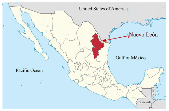
Figure 1.
The state of Nuevo León is highlighted for reference. Geographical places of interest are named for reference as well. The image was taken and modified from the work in [19].
It is intended that this research will allow evaluating the viability of implementation of solar projects in this zone, as well as establishing methods of estimating the solar irradiation in other areas using the same program. This data source was selected due to its reliability and access to data worldwide for the parameters required for the calculations in the model utilized in this research and as a reference for comparison against data obtained from the model during the validation for the analyzed geographic zone. In addition, this data source contains a collection of around 30 years of several meteorological parameters based on satellite observation. This provides a solid comparison reference for validation of the model.
Inside the main page of The Power Project, select the option POWER DATA ACCESS VIEWER, and a map will be displayed. In the floating menu, select the Climatology option and enter the desired latitude and longitude, along with the parameters of interest. With this, the database provides the required data [16]. For the current research, clearness index () and surface albedo () were obtained from the database for the calculations as well as all sky insolation incident on a horizontal surface (G) for validation of the model.
Note that other data sources such as meteorological stations from the Mexican national meteorological system (SMN) were considered but discarded due to the lack of stations in the state of Nuevo León (only three stations), which was considered not enough for comparison.
3. Methodology
This section presents the research methodology that was followed to obtain a GIS analysis, which reflects the yearly behavior of the total insolation as well as the maximum and minimum temperatures in the state of Nuevo León, Mexico. Besides, all the process related to the validation of the model employed and the design of a representative grid are illustrated for the state of Nuevo León. The applied methodology is presented in Figure 2.
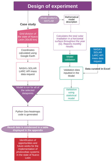
Figure 2.
Applied methodology.
3.1. Mathematical Model
The work reported by Enríquez-Velásquez et al. [14] was based on the mathematical model developed by Obukhov et al. [15] for high latitudes (55° N). This model was applied in [14] for the calculation and evaluation of the solar resource in the Northwestern Mexican state of Sonora at latitudes between 26° and 32° N. The applied mathematical formula for the estimation of total solar irradiation arriving at an inclined surface (G) is as follows:
Equation (1) presents the calculation of the total solar irradiation on a surface orientated at any angle, it adds the direct, diffuse, and reflective components of solar radiation for calculation. The model includes the tilt angle of the receiving surface (), the surface albedo (), the incidence angle (), the solar zenith angle (), and the anisotropic index (). Other parameters such as the diffusion index were calculated using the conditional table reported in [14]. For further information on the calculation of each variable, the same document can be consulted.
Table 1 shows the day taken to represent a reliable average representation of solar irradiation for each month. In addition, the model was used to calculate the average monthly solar irradiance on a horizontal surface throughout the year. The above-mentioned model was written in MATLAB and was instructed to read the input data from an Excel file containing the pertaining data of all the chosen geographical points of interest, and once every calculation was made, it outputted the resulting data in a second Excel file for further processing of the data. Furthermore, additional input data to run the mathematical model were obtained with the use of Python code requesting mass data from NASA’s POWER LARC API. These data were produced as several CSV files that were later merged using Excel data manipulation tools for them to be readable by the model.

Table 1.
Average representative day for each month.
In this research, 80 geographic coordinates were fed to the program at once. The program calculations took around 90 min to complete for the millions of required calculations for several geographical points. This represents a significant advantage over calculating each data point manually or retrieving all the several results and parameters from a database. The mathematical model presents a clear advantage of calculating several geographical data points at once and generates an Excel file with the results in an acceptable period of time.
3.2. Statistical Parameters
To validate the model, pertinent statistical methods were used to ensure data accuracy. The data generated using the herein mathematical model were compared against the data provided by NASA SSE project [16], specifically for “Total radiation arriving at a horizontal surface” parameter G. The eight statistical methods employed are outlined in Equations (2)–(9), where stands for each G-value calculated by the mathematical model, is the G-value provided by NASA’s SSE database, n is the number of months (sample size), and i represents the month number analyzed.
MAE—Mean absolute error
In Equation (2), mean absolute error (MAE) represents the average of the error’s magnitude. It is desired for this value to be as close to zero as possible. MAE calculates a ratio relating the number of samples n to the magnitude of the error vector [20].
MBE—Mean bias error
In Equation (3), mean bias error (MBE) calculates the bias of the model results. For this value, the closer it is to zero, the better [21].
RMSE—Root mean square error
In Equation (4), root mean square error (RMSE) calculates the standard deviation of the calculated data [22]. It is desired to be as close to zero as possible.
MPE—Mean percentage error
In Equation (5), mean percentage error (MPE) calculates the percentage of the error in the model calculated data, it is used to describe the performance of the error. A value is allowable [23].
RPE—Relative percentage error
Equation (6) calculated the relative percentage error (RPE) that represents the percentage of error for each of monthly results. A value is permissible [24].
r—Correlation coefficient
In Equation (7), r (correlation coefficient) indicates the correlation between two different variables in a range of , where is a positive linear correlation, represents a negative linear correlation, and 0 stands for no correlation at all. Correlation vales are desired to be as close to 1 as possible. Moreover, represents the annual average G-value calculated using the mathematical model, and is the annual average G-value provided by the NASA SSE database [25].
—Coefficient of determination
In Equation (8), the coefficient of determination, , determines the percentage of variability between the results of the model and data set used, particularly in calculating the adequacy of the model to explain the variations represented with a value from 0 to 1. It is desired for to be as close to 1 as possible [26].
t—Student distribution test
As presented in Equation (9), the t—Student distribution test is commonly used to relate the significance of two independent data sets, and it is specifically useful when dealing with a small sample size (small value of n, in this case, 12 months). This statistical test shows if a value shows statistical significance according to selected metrics. For this test, a critical value of was chosen to reflect a confidence level of and eleven degrees-of-freedom. In the formula, MBE represents the Mean bias error, RMSE represents the Root mean square error, df stands for degrees of freedom, and n is the number of months calculated. To prove statistical significance, the calculated t-value must be less than the chosen critical value [27].
3.3. Model Validation
The NASA SSE data were used to validate the model’s results for each of the five chosen locations by evaluating that these results coincide with, or approximate, the data obtained by NASA SSE. Statistical models were calculated to analyze the performance of the model compared to the data source. The model was validated using these strategic points scattered at the edges of the Mexican state of Nuevo León under the premise of having an overview of the model behavior under the most extreme parameter conditions available in this territory.
The five points were chosen to represent the cardinal points in the state. They were placed as follows: Monterrey city to the west, China represents a point in the center of the state, Osca town to the East, Doctor Arroyo to the South, and Anáhuac to the North. This deployment allowed more diverse data to be used for validation of the model, something that would not have been possible if Mexico’s Meteorological Service’s data had been used instead. The latitudes and longitudes of the five locations are listed in Table 2.
Table 2.
Latitude and longitude coordinates for all five locations in the state of Nuevo León chosen as reference points to validate the mathematical model with NASA’s data.
The calculated validation data were processed using several statistical methods to ensure their significance and accuracy by comparing them to NASA’s long-term acquired data. This comparison was further explored by plotting them side-by-side using MATLAB functions.
3.4. Area Justification
To create a visual representation of the temperatures and solar radiation in the delimited surface, a grid was created to generate heat maps for the whole state. The Tech District, the area around the Monterrey tech campus, was selected as the origin point of this grid, i.e., the rounded red-black point to the right of as shown in Figure 3. This is because the location is of special interest for future research on solar energy, and a meteorological facility is in the process to be installed in this area. The grid was generated from this point using axes parallel to the equator and the Greenwich Meridian, respectively. Each grid cell is composed of a 30 km-sided square, using the vertices of each cell as evaluation points for the desired data (maximum temperature, minimum temperature, or solar irradiation); thus, 80 of these points were produced around the state of Nuevo León. The 30 km × 30 km grid resolution was used to prevent retrieving too many data points, but at the same time providing acceptable results (supported by the statistical validation and comparison against NASA SEE database). A higher resolution (with lower length for each cell side) is not convenient as, if vertices are too close to each other, solar radiation will vary little between them. Figure 3 and Figure 4 illustrate the work done in Google Earth software to distribute the 80 points and to draw the grid to cover all the surface of the state.
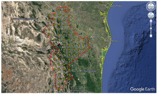
Figure 3.
Geographical points (80 in total) selected for mathematical model calculation. The rounded red-black point represents the grid’s origin.
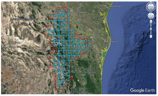
Figure 4.
The resulting grid strategically dividing the state of Nuevo León. The lines are parallel to the equator and Greenwich Meridian.
3.5. Heat Maps
GIS maps are used to determine the amount of solar resource on a certain surface. The total solar radiation was calculated for each point on the statewide grid for each month of the year. Average maximum and minimum monthly temperatures were taken from the NASA SSE data source for each point as a comparison reference. The model was run in these chosen locations in the grid. The results were then plotted in several heatmaps to provide an overview of the annual variation in solar irradiance arriving at a horizontal surface throughout the state’s territory.
The heatmaps were coded in Python with support of Pandas and Plotly libraries. The Pandas library was used for data manipulation. The Plotly library was employed to fetch maps and generate a heatmap on top of it, adding its corresponded legends and color bar. At last, Kaleido library was employed to generate a resulting vectorized image for further enhancement and postprocessing.
4. Results and Discussion
This section presents the results obtained in the research and discuss the findings to develop an identification of opportunities and potential for solar energy in the state of Nuevo León based on the results.
4.1. Model Validation Results
The mathematical model was analyzed for the five locations presented in Section 3, which were selected in the state of Nuevo León to represent its surface. These points were selected for each cardinal and one in the middle of the state to ensure the maximum coverage possible. Based on these points, a validation comparing the model against the NASA SSE database using the statistical parameters presented in Section 3 was realized.
The results obtained from the above-mentioned analysis were satisfactory for all the cases and just small discrepancies were observed. Noticed values for MAE, MBE, and RMSE were close to zero for almost all cases, which means minimum errors presented between the model and the reference. Slightly higher values of these parameters were shown in the cases of China and Anahuac, but they remain acceptable.
For MPE and RPE tests values close to zero percent were obtained for all localities, which means all cases were on an acceptable range. It was found positive linear correlation for all cases using the parameter “r”. Furthermore, for tests, the best performance was presented in Dr. Arroyo and La Osca, followed by Monterrey and Anahuac, a smaller performance but still acceptable was observed in China.
The t-distribution test illustrates four of the analyzed points as statistically significant, the only exception was Anahuac which remained a little high respect to the critical point selected. Based on the realized statistical results, it was observed that the model is a very close approximation to the values obtained from the NASA SSE database. This proves that the model is a valid estimation of solar irradiation in the geographical coordinates of the state of Nuevo León. Table 3 and Table 4 provide all the monthly calculations for solar irradiation obtained from the model and the reference from NASA SSE. Additionally, it shows the values obtained for all the statistical metrics analyzed. To review the accuracy of results, refer to the statistical parameters in Section 3.2.
Table 3.
Monthly comparison of G from the model against the G provided by NASA SSE database for the five target points.
Table 4.
Statistical parameters to measure quality of estimated G against G from NASA SSE database for the five target points.
Figure 5, Figure 6, Figure 7, Figure 8 and Figure 9 illustrate the behavior of the model respect to the values from the NASA SSE database. The values shown in Figure 5, Figure 6, Figure 7, Figure 8 and Figure 9 are in kWh/m2 for solar irradiation. It can be observed that for La Osca, the model and the NASA SSE values were nearly identical for all months, then for Dr. Arroyo and Monterrey small discrepancies were observed in certain months. Finally, the biggest differences were found in Anáhuac and China for the summer months, but these differences remain small.
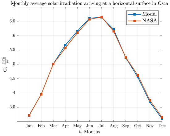
Figure 5.
Values obtained for La Osca from mathematical model and NASA SSE.
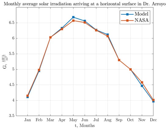
Figure 6.
Values obtained for Doctor Arroyo from mathematical model and NASA SSE.
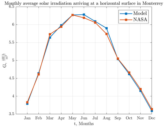
Figure 7.
Values obtained for Monterrey from mathematical model and NASA SSE.
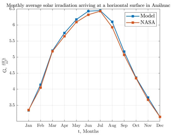
Figure 8.
Values obtained for Anáhuac from mathematical model and NASA SSE.
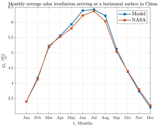
Figure 9.
Values obtained for China from mathematical model and NASA SSE.
4.2. GIS Analysis Results
From the GIS analysis applied to the grid described in Section 3 for strategical points to calculate solar irradiation in Nuevo León, it was found that the minimum value during the year for all the state surface was kWh/m2 and reached a maximum value of kWh/m2 in the analysis of the points studied. This illustrates the availability of solar resource in the states and its evolution throughout the year. As a result, for the 12 months of the year, the GIS of average total solar irradiation at a horizontal surface, the average of the maximum temperatures, and the average of the minimum temperatures are presented in Figure 10, Figure 11, Figure 12, Figure 13, Figure 14, Figure 15, Figure 16, Figure 17, Figure 18, Figure 19, Figure 20 and Figure 21. These GIS were generated from the computations in Appendix A.
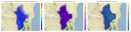
Figure 10.
GIS analysis for the month of January. (left) Average solar irradiation (kWh/m2), (center) Maximum average temperature (°C), and (right) Minimum average temperature (°C).
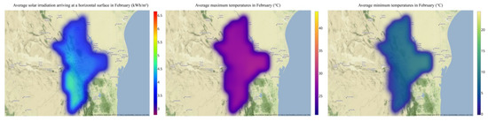
Figure 11.
GIS analysis for the month of February. (left) Average solar irradiation (kWh/m2), (center) Maximum average temperature (°C), and (right) Minimum average temperature (°C).
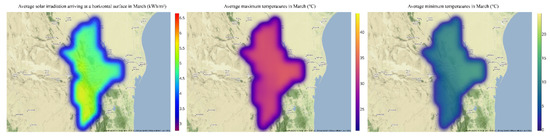
Figure 12.
GIS analysis for the month of March. (left) Average solar irradiation (kWh/m2), (center) Maximum average temperature (°C), and (right) Minimum average temperature (°C).
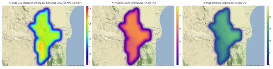
Figure 13.
GIS analysis for the month of April. (left) Average solar irradiation (kWh/m2), (center) Maximum average temperature (°C), and (right) Minimum average temperature (°C).
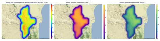
Figure 14.
GIS analysis for the month of May. (left) Average solar irradiation (kWh/m2), (center) Maximum average temperature (°C), and (right) Minimum average temperature (°C).
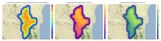
Figure 15.
GIS analysis for the month of June. (left) Average solar irradiation (kWh/m2), (center) Maximum average temperature (°C), and (right) Minimum average temperature (°C).
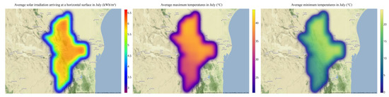
Figure 16.
GIS analysis for the month of July. (left) Average solar irradiation (kWh/m2), (center) Maximum average temperature (°C), and (right) Minimum average temperature (°C).
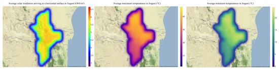
Figure 17.
GIS analysis for the month of August. (left) Average solar irradiation (kWh/m2), (center) Maximum average temperature (°C), and (right) Minimum average temperature (°C).
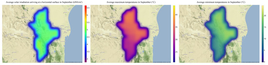
Figure 18.
GIS analysis for the month of September. (left) Average solar irradiation (kWh/m2), (center) Maximum average temperature (°C), and (right) Minimum average temperature (°C).
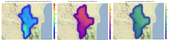
Figure 19.
GIS analysis for the month of October. (left) Average solar irradiation (kWh/m2), (center) Maximum average temperature (°C), and (right) Minimum average temperature (°C).
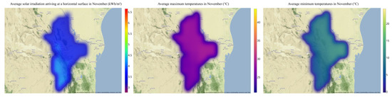
Figure 20.
GIS analysis for the month of November. (left) Average solar irradiation (kWh/m2), (center) Maximum average temperature (°C), and (right) Minimum average temperature (°C).
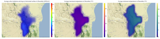
Figure 21.
GIS analysis for the month of December. (left) Average solar irradiation (kWh/m2), (center) Maximum average temperature (°C), and (right) Minimum average temperature (°C).
The identified zone with the most constant solar irradiation levels during the year was south-west of the state, except for the months of June–August, where solar irradiation passes to be almost constant in the whole state but with slightly higher values in the north and east of the state in June and July. The average maximum and minimum temperatures for the state fluctuate in a range from 1.55 °C to 43.84 °C during the year for all the points analyzed.
The highest temperatures were found in the northern and eastern regions, whereas the lowest are in the south and west. On the other hand, the state contains mountainous terrain in its southern and western areas, passing to plains in its northern and eastern regions. All the previous factors must be considered in planning PV projects. Based on the previous factors, it was found that the west region where the capital city of Monterrey is located appears promising on average throughout the year for values of total solar irradiance. However, the effect of low and high temperatures on photovoltaic systems must be taken into account to realize the proper design for solar projects considering the effects of extreme temperatures on solar PV panels (current and voltage). An advantage of the state in terms of minimum temperatures is that there are no sub-zero temperatures, which facilitates the design and selection of components of a photovoltaic system, by not leading to such large variations in voltage due to temperature change.
A factor to consider for the west and south zones of the state is that the terrain is mountainous, which makes it difficult to implement large-scale photovoltaic projects due to space and suitable terrain issues. This is because of the space required to avoid shadowing and the right distribution of solar panels in the terrain; the bigger the project, the most terrain it will require. On the other hand, north and east regions are defined by plain terrain, which allows development of large-scale PV projects. Here, the main issue is maximum temperatures in summer, which reduce efficiency in the energy conversion from PV panels, so measures to counteract these effects must be taken in the design.
The GIS analysis applied to solar irradiation proves itself a useful tool that allows easy identification of opportunity areas for photovoltaic systems in the state of Nuevo León. The main advantage is that all information required for decision-making is shown, comparing parameters which affect PV performance and planning, such as temperatures and geographical terrain. It is important to consider the proper resolution for the analyzed area. As explained in Section 3, a distribution of points on a grid of 30 × 30 km was defined.
Compared against the approach applied by Enríquez-Velásquez et al. [14], the approach herein has the improvement of using a grid to divide the area of interest, instead of dividing the surface into municipalities, which have irregular shapes, as it was done in the state of Sonora, Mexico. The grid concept is versatile and allows to estimate, in a more uniform way, the solar resource of any area, taking a given latitude and longitude as the origin point of the grid. It should also be considered that the mathematical model will need to be validated if it is going to be applied to other latitudes and longitudes as suggested by Kausika et al. [11].
5. Conclusions and Future Work
Based on the findings previously described in Section 4, it is concluded that the mathematical model utilized in this research work was successful for computing total solar irradiation and demonstrated high accuracy values for the state of Nuevo León in México. This accuracy was proved using statistical metrics comparing the model against the NASA SSE database as reference. The validation of the model was tested for the geographic zone between latitudes from 28° to 23° N and longitudes from 98° to 101° W.
Based on a scrutiny of the state of Nuevo León using GIS analysis, the solar irradiation calculated by the model was compared against maximum and minimum temperatures, and opportunities for local photovoltaic (PV) development were identified. The GIS analysis was realized over a grid of 30 × 30 km, which covers the totality of the state surface. This approach allowed a clear visualization of the solar irradiation, without rejecting data due to long distances between the points of the grid proposed. It was concluded that solar irradiation in the state of Nuevo León ranges from kWh/m2 to kWh/m2, as minimum and maximum ranges. This result demonstrated the high potential of solar energy projects in the region. The comparison against extreme temperatures and geographical terrain allowed to point certain areas in the region, which are more suitable for PV development.
It was also inferred that the most suitable zones for solar collecting systems may be located in the southwest, which presented constant solar irradiation values throughout the year; however, these zones are mountainous, so it should be considered in the design of solar farms due to space requirements to avoid shadowing among solar panels. Note that the most industrialized zone of the state is located in the Monterrey metropolitan area, and it presents constant solar irradiation throughout the year, which represents great potential for the sustainable development of the industrial base in the city.
This would result in greatly reducing the carbon emissions of the state, which is one of the most industrialized in Mexico. As a result, this region would contribute towards the accomplishment of Mexico’s international agreements in relation to the reduction of its carbon footprint and commitments such as the Paris Agreement. This would be reflected in urbanization and sustainable development in electricity generation for the city of Monterrey. The mathematical model used in this research is shown to be an easy and accurate tool to estimate solar irradiation in the region, with the ease of not depending on field references for the calculations, and only requires meteorological data and geographic coordinates easily accessible online.
This represents an economical alternative compared to meteorological stations that require constant maintenance and cost of implementation. In addition to these factors, it should be considered that a large number of meteorological stations must be available to cover the entire area of the state for the same resolution obtained by the model. Considering all the previous factors, it is concluded that the proposed model and GIS analysis offer a great opportunity for solar energy planning in the public and private sectors in the state, and to used these GIS methods as decision-making tools and reference for the implementation of solar projects in the region. Furthermore, a tool for a possible cooperation with the United States regarding sustainable development of both nations.
As future work, the application of the model is proposed by implementing different inclination angles for the receiving surface, as well as surface azimuth to simulate the daily tracking of the sun throughout the year. Besides, more databases for solar resource estimation may be employed to reinforce the validation of our results. This would be the basis for developing a solar monitoring system that would increase the efficiency of solar collection in PV systems within the region, and thus, increasing their profitability and production of electrical energy. Additionally, solar tracking could be used to design arrays of heliostats to focus sunlight at a central tower to heat liquids and generate steam for electric generation using solar thermal technologies. These projects are focused on sustainable urban and industrial development facing the current challenges of climate change.
Author Contributions
Conceptualization, E.A.E.-V. and J.d.-J.L.-S.; methodology, E.A.E.-V., L.C.F.-H. and V.H.B.; software, F.A.V.-D.; validation, F.A.V.-D., L.A.S.C., E.A.E.-V. and L.C.F.-H.; formal analysis, F.A.V.-D., L.A.S.C. and E.A.E.-V.; investigation, F.A.V.-D., L.A.S.C., E.A.E.-V., L.C.F.-H. and V.H.B.; resources, J.d.-J.L.-S.; data curation, F.A.V.-D. and E.A.E.-V.; writing-original draft preparation, F.A.V.-D., L.A.S.C., E.A.E.-V. and L.C.F.-H.; writing—review and editing V.H.B., J.d.-J.L.-S. and R.A.R.-M.; visualization, V.H.B., J.d.-J.L.-S. and R.A.R.-M.; supervision, L.C.F.-H.; project administration, L.C.F.-H.; funding acquisition, J.d.-J.L.-S. and R.A.R.-M. All authors have read and agreed to the published version of the manuscript.
Funding
The APC was funded by CampusCity Initiative from the School of Engineering and Sciences at the Tecnologico de Monterrey.
Acknowledgments
The authors are grateful to Tecnológico de Monterrey for having provided the software resources to carry out the simulation work. In addition, we thank NASA—The Power Project for giving free access to its databases and to consult the reference values to estimate the total solar irradiation and corroborate the results.
Conflicts of Interest
The authors declare no conflict of interest. The funder had no role in the design of the study; in the collection, analyses, or interpretation of data; in the writing of the manuscript; or in the decision to publish the results.
Appendix A
Solar Irradiance Parameters for the 80 Selected Points in the State of Nuevo León
Table A1.
Monthly parameter measurements for each point on the state-wide grid.
Table A1.
Monthly parameter measurements for each point on the state-wide grid.
| Location | LAT | LON | Parameter | January | February | March | April | May | June | July | August | September | October | November | December | Annual Average |
|---|---|---|---|---|---|---|---|---|---|---|---|---|---|---|---|---|
| D. Tec | 25.6544° | −100.2871° | G_Model | 3.79 | 4.64 | 5.64 | 5.98 | 6.27 | 6.28 | 6.09 | 5.9 | 5.04 | 4.62 | 4.15 | 3.59 | 5.17 |
| G_NASA | 3.83 | 4.61 | 5.73 | 5.94 | 6.27 | 6.19 | 6.06 | 5.74 | 5.05 | 4.66 | 4.2 | 3.64 | 5.16 | |||
| SRF_ALB | 0.15 | 0.14 | 0.15 | 0.14 | 0.15 | 0.16 | 0.15 | 0.16 | 0.15 | 0.13 | 0.13 | 0.15 | 0.15 | |||
| KT | 0.58 | 0.6 | 0.62 | 0.58 | 0.57 | 0.56 | 0.55 | 0.56 | 0.53 | 0.57 | 0.61 | 0.58 | 0.58 | |||
| TS_MAX | 25.32 | 29.09 | 33.96 | 38.27 | 40.54 | 40.39 | 39.07 | 38.73 | 34.64 | 32.16 | 28.52 | 25.17 | 33.82 | |||
| TS_MIN | 5.07 | 6.96 | 9.97 | 14.2 | 17.87 | 19.46 | 19.15 | 19.31 | 17.54 | 13.68 | 9.16 | 5.8 | 13.18 | |||
| A1 | 25.9252° | −100.2871° | G_Model | 3.77 | 4.62 | 5.63 | 5.98 | 6.27 | 6.29 | 6.09 | 5.9 | 5.03 | 4.61 | 4.13 | 3.56 | 5.16 |
| G_NASA | 3.83 | 4.61 | 5.73 | 5.94 | 6.27 | 6.19 | 6.06 | 5.74 | 5.05 | 4.66 | 4.2 | 3.64 | 5.16 | |||
| SRF_ALB | 0.15 | 0.14 | 0.15 | 0.14 | 0.15 | 0.16 | 0.15 | 0.16 | 0.15 | 0.13 | 0.13 | 0.15 | 0.15 | |||
| KT | 0.58 | 0.6 | 0.62 | 0.58 | 0.57 | 0.56 | 0.55 | 0.56 | 0.53 | 0.57 | 0.61 | 0.58 | 0.58 | |||
| TS_MAX | 25.32 | 29.09 | 33.96 | 38.27 | 40.54 | 40.39 | 39.07 | 38.73 | 34.64 | 32.16 | 28.52 | 25.17 | 33.82 | |||
| TS_MIN | 5.07 | 6.96 | 9.97 | 14.2 | 17.87 | 19.46 | 19.15 | 19.31 | 17.54 | 13.68 | 9.16 | 5.8 | 13.18 | |||
| A2 | 26.196° | −100.2871° | G_Model | 3.49 | 4.29 | 5.34 | 5.77 | 6.17 | 6.41 | 6.21 | 5.9 | 5.02 | 4.43 | 3.83 | 3.36 | 5.02 |
| G_NASA | 3.44 | 4.21 | 5.29 | 5.65 | 6.11 | 6.17 | 6.15 | 5.71 | 4.93 | 4.38 | 3.79 | 3.28 | 4.93 | |||
| SRF_ALB | 0.15 | 0.15 | 0.16 | 0.15 | 0.16 | 0.17 | 0.16 | 0.17 | 0.17 | 0.14 | 0.14 | 0.15 | 0.16 | |||
| KT | 0.54 | 0.56 | 0.59 | 0.56 | 0.56 | 0.57 | 0.56 | 0.56 | 0.53 | 0.55 | 0.57 | 0.55 | 0.56 | |||
| TS_MAX | 25.18 | 29.31 | 34.63 | 39.31 | 41.99 | 42.29 | 41.06 | 40.87 | 36.6 | 33.8 | 29.16 | 25.04 | 34.94 | |||
| TS_MIN | 5.7 | 7.82 | 11.2 | 15.55 | 19.62 | 21.64 | 21.45 | 21.67 | 19.58 | 15.38 | 10.3 | 6.42 | 14.69 | |||
| A3 | 26.4668° | −100.2871° | G_Model | 3.46 | 4.27 | 5.33 | 5.76 | 6.17 | 6.41 | 6.22 | 5.9 | 5.01 | 4.41 | 3.81 | 3.33 | 5.01 |
| G_NASA | 3.44 | 4.21 | 5.29 | 5.65 | 6.11 | 6.17 | 6.15 | 5.71 | 4.93 | 4.38 | 3.79 | 3.28 | 4.93 | |||
| SRF_ALB | 0.15 | 0.15 | 0.16 | 0.15 | 0.16 | 0.17 | 0.16 | 0.17 | 0.17 | 0.14 | 0.14 | 0.15 | 0.16 | |||
| KT | 0.54 | 0.56 | 0.59 | 0.56 | 0.56 | 0.57 | 0.56 | 0.56 | 0.53 | 0.55 | 0.57 | 0.55 | 0.56 | |||
| TS_MAX | 25.18 | 29.31 | 34.63 | 39.31 | 41.99 | 42.29 | 41.06 | 40.87 | 36.6 | 33.8 | 29.16 | 25.04 | 34.94 | |||
| TS_MIN | 5.7 | 7.82 | 11.2 | 15.55 | 19.62 | 21.64 | 21.45 | 21.67 | 19.58 | 15.38 | 10.3 | 6.42 | 14.69 | |||
| A4 | 26.7375° | −100.2871° | G_Model | 3.44 | 4.25 | 5.31 | 5.76 | 6.17 | 6.42 | 6.22 | 5.89 | 5 | 4.39 | 3.79 | 3.31 | 5 |
| G_NASA | 3.44 | 4.21 | 5.29 | 5.65 | 6.11 | 6.17 | 6.15 | 5.71 | 4.93 | 4.38 | 3.79 | 3.28 | 4.93 | |||
| SRF_ALB | 0.15 | 0.15 | 0.16 | 0.15 | 0.16 | 0.17 | 0.16 | 0.17 | 0.17 | 0.14 | 0.14 | 0.15 | 0.16 | |||
| KT | 0.54 | 0.56 | 0.59 | 0.56 | 0.56 | 0.57 | 0.56 | 0.56 | 0.53 | 0.55 | 0.57 | 0.55 | 0.56 | |||
| TS_MAX | 24.9 | 29.23 | 34.88 | 39.64 | 42.35 | 43.17 | 42.17 | 42.13 | 37.76 | 34.73 | 29.43 | 24.72 | 35.43 | |||
| TS_MIN | 5.71 | 7.94 | 11.58 | 16 | 20.26 | 22.64 | 22.6 | 22.91 | 20.53 | 16.05 | 10.67 | 6.43 | 15.28 | |||
| A5 | 27.0083° | −100.2871° | G_Model | 3.35 | 4.15 | 5.21 | 5.75 | 6.17 | 6.43 | 6.45 | 6.1 | 5.18 | 4.37 | 3.76 | 3.16 | 5.01 |
| G_NASA | 3.35 | 4.05 | 5.18 | 5.65 | 6.09 | 6.32 | 6.43 | 5.93 | 5.07 | 4.34 | 3.67 | 3.14 | 4.93 | |||
| SRF_ALB | 0.16 | 0.16 | 0.16 | 0.16 | 0.16 | 0.17 | 0.17 | 0.18 | 0.17 | 0.15 | 0.15 | 0.15 | 0.16 | |||
| KT | 0.53 | 0.55 | 0.58 | 0.56 | 0.56 | 0.57 | 0.58 | 0.58 | 0.55 | 0.55 | 0.57 | 0.53 | 0.56 | |||
| TS_MAX | 24.65 | 29.17 | 34.91 | 39.61 | 42.25 | 43.65 | 42.9 | 43.08 | 38.64 | 35.24 | 29.54 | 24.45 | 35.67 | |||
| TS_MIN | 5.92 | 8.28 | 12.13 | 16.6 | 20.96 | 23.63 | 23.74 | 24.14 | 21.43 | 16.76 | 11.16 | 6.67 | 15.95 | |||
| A6 | 27.279° | −100.2871° | G_Model | 3.33 | 4.13 | 5.19 | 5.75 | 6.18 | 6.43 | 6.45 | 6.1 | 5.17 | 4.35 | 3.74 | 3.14 | 5 |
| G_NASA | 3.35 | 4.05 | 5.18 | 5.65 | 6.09 | 6.32 | 6.43 | 5.93 | 5.07 | 4.34 | 3.67 | 3.14 | 4.93 | |||
| SRF_ALB | 0.16 | 0.16 | 0.16 | 0.16 | 0.16 | 0.17 | 0.17 | 0.18 | 0.17 | 0.15 | 0.15 | 0.15 | 0.16 | |||
| KT | 0.53 | 0.55 | 0.58 | 0.56 | 0.56 | 0.57 | 0.58 | 0.58 | 0.55 | 0.55 | 0.57 | 0.53 | 0.56 | |||
| TS_MAX | 24.65 | 29.17 | 34.91 | 39.61 | 42.25 | 43.65 | 42.9 | 43.08 | 38.64 | 35.24 | 29.54 | 24.45 | 35.67 | |||
| TS_MIN | 5.92 | 8.28 | 12.13 | 16.6 | 20.96 | 23.63 | 23.74 | 24.14 | 21.43 | 16.76 | 11.16 | 6.67 | 15.95 | |||
| A7 | 27.5498° | −100.2871° | G_Model | 3.31 | 4.11 | 5.18 | 5.74 | 6.18 | 6.44 | 6.46 | 6.1 | 5.16 | 4.34 | 3.72 | 3.12 | 4.99 |
| G_NASA | 3.35 | 4.05 | 5.18 | 5.65 | 6.09 | 6.32 | 6.43 | 5.93 | 5.07 | 4.34 | 3.67 | 3.14 | 4.93 | |||
| SRF_ALB | 0.16 | 0.16 | 0.16 | 0.16 | 0.16 | 0.17 | 0.17 | 0.18 | 0.17 | 0.15 | 0.15 | 0.15 | 0.16 | |||
| KT | 0.53 | 0.55 | 0.58 | 0.56 | 0.56 | 0.57 | 0.58 | 0.58 | 0.55 | 0.55 | 0.57 | 0.53 | 0.56 | |||
| TS_MAX | 23.98 | 28.54 | 34.21 | 38.9 | 41.48 | 43.4 | 42.93 | 43.39 | 39 | 35.02 | 29 | 23.8 | 35.3 | |||
| TS_MIN | 5.5 | 7.94 | 11.84 | 16.32 | 20.76 | 23.67 | 23.96 | 24.44 | 21.47 | 16.59 | 10.87 | 6.28 | 15.8 |
Table A2.
Monthly parameter measurements for each point on the state-wide grid.
Table A2.
Monthly parameter measurements for each point on the state-wide grid.
| Location | LAT | LON | Parameter | January | February | March | April | May | June | July | August | September | October | November | December | Annual Average |
|---|---|---|---|---|---|---|---|---|---|---|---|---|---|---|---|---|
| A-1 | 25.3836° | −100.2871° | G_Model | 3.82 | 4.66 | 5.66 | 5.99 | 6.27 | 6.27 | 6.09 | 5.9 | 5.05 | 4.64 | 4.18 | 3.61 | 5.18 |
| G_NASA | 3.83 | 4.61 | 5.73 | 5.94 | 6.27 | 6.19 | 6.06 | 5.74 | 5.05 | 4.66 | 4.2 | 3.64 | 5.16 | |||
| SRF_ALB | 0.15 | 0.14 | 0.15 | 0.14 | 0.15 | 0.16 | 0.15 | 0.16 | 0.15 | 0.13 | 0.13 | 0.15 | 0.15 | |||
| KT | 0.58 | 0.6 | 0.62 | 0.58 | 0.57 | 0.56 | 0.55 | 0.56 | 0.53 | 0.57 | 0.61 | 0.58 | 0.58 | |||
| TS_MAX | 24.46 | 27.81 | 32.26 | 36.09 | 37.9 | 37.3 | 35.92 | 35.48 | 31.95 | 29.91 | 27.08 | 24.33 | 31.71 | |||
| TS_MIN | 3.78 | 5.35 | 7.96 | 11.92 | 15.15 | 16.35 | 15.99 | 16.05 | 14.65 | 11.29 | 7.42 | 4.54 | 10.87 | |||
| A-2 | 25.1128° | −100.2871° | G_Model | 3.84 | 4.68 | 5.67 | 5.99 | 6.26 | 6.27 | 6.08 | 5.9 | 5.06 | 4.66 | 4.2 | 3.64 | 5.19 |
| G_NASA | 3.83 | 4.61 | 5.73 | 5.94 | 6.27 | 6.19 | 6.06 | 5.74 | 5.05 | 4.66 | 4.2 | 3.64 | 5.16 | |||
| SRF_ALB | 0.15 | 0.14 | 0.15 | 0.14 | 0.15 | 0.16 | 0.15 | 0.16 | 0.15 | 0.13 | 0.13 | 0.15 | 0.15 | |||
| KT | 0.58 | 0.6 | 0.62 | 0.58 | 0.57 | 0.56 | 0.55 | 0.56 | 0.53 | 0.57 | 0.61 | 0.58 | 0.58 | |||
| TS_MAX | 24.46 | 27.81 | 32.26 | 36.09 | 37.9 | 37.3 | 35.92 | 35.48 | 31.95 | 29.91 | 27.08 | 24.33 | 31.71 | |||
| TS_MIN | 3.78 | 5.35 | 7.96 | 11.92 | 15.15 | 16.35 | 15.99 | 16.05 | 14.65 | 11.29 | 7.42 | 4.54 | 10.87 | |||
| A-3 | 24.842° | −100.2871° | G_Model | 4 | 4.86 | 5.87 | 6.31 | 6.59 | 6.59 | 6.3 | 6.12 | 5.36 | 4.92 | 4.36 | 3.92 | 5.43 |
| G_NASA | 4.06 | 4.85 | 5.9 | 6.24 | 6.52 | 6.48 | 6.28 | 6.01 | 5.3 | 4.94 | 4.46 | 3.93 | 5.41 | |||
| SRF_ALB | 0.16 | 0.16 | 0.17 | 0.17 | 0.17 | 0.18 | 0.17 | 0.17 | 0.17 | 0.15 | 0.15 | 0.16 | 0.16 | |||
| KT | 0.6 | 0.62 | 0.64 | 0.61 | 0.6 | 0.59 | 0.57 | 0.58 | 0.56 | 0.6 | 0.63 | 0.62 | 0.6 | |||
| TS_MAX | 24.15 | 27.47 | 31.79 | 35.5 | 37.13 | 36.09 | 34.43 | 33.94 | 30.84 | 29.18 | 26.59 | 24.07 | 30.93 | |||
| TS_MIN | 3.21 | 4.62 | 7.02 | 10.74 | 13.7 | 14.72 | 14.26 | 14.23 | 13.07 | 10.1 | 6.6 | 4.01 | 9.69 | |||
| A-4 | 24.5711° | −100.2871° | G_Model | 4.03 | 4.88 | 5.89 | 6.31 | 6.58 | 6.59 | 6.29 | 6.12 | 5.37 | 4.94 | 4.39 | 3.94 | 5.44 |
| G_NASA | 4.06 | 4.85 | 5.9 | 6.24 | 6.52 | 6.48 | 6.28 | 6.01 | 5.3 | 4.94 | 4.46 | 3.93 | 5.41 | |||
| SRF_ALB | 0.16 | 0.16 | 0.17 | 0.17 | 0.17 | 0.18 | 0.17 | 0.17 | 0.17 | 0.15 | 0.15 | 0.16 | 0.16 | |||
| KT | 0.6 | 0.62 | 0.64 | 0.61 | 0.6 | 0.59 | 0.57 | 0.58 | 0.56 | 0.6 | 0.63 | 0.62 | 0.6 | |||
| TS_MAX | 24.15 | 27.47 | 31.79 | 35.5 | 37.13 | 36.09 | 34.43 | 33.94 | 30.84 | 29.18 | 26.59 | 24.07 | 30.93 | |||
| TS_MIN | 3.21 | 4.62 | 7.02 | 10.74 | 13.7 | 14.72 | 14.26 | 14.23 | 13.07 | 10.1 | 6.6 | 4.01 | 9.69 | |||
| A-5 | 24.3003° | −100.2871° | G_Model | 4.05 | 4.9 | 5.9 | 6.32 | 6.58 | 6.58 | 6.28 | 6.12 | 5.38 | 4.96 | 4.42 | 3.97 | 5.46 |
| G_NASA | 4.06 | 4.85 | 5.9 | 6.24 | 6.52 | 6.48 | 6.28 | 6.01 | 5.3 | 4.94 | 4.46 | 3.93 | 5.41 | |||
| SRF_ALB | 0.16 | 0.16 | 0.17 | 0.17 | 0.17 | 0.18 | 0.17 | 0.17 | 0.17 | 0.15 | 0.15 | 0.16 | 0.16 | |||
| KT | 0.6 | 0.62 | 0.64 | 0.61 | 0.6 | 0.59 | 0.57 | 0.58 | 0.56 | 0.6 | 0.63 | 0.62 | 0.6 | |||
| TS_MAX | 24.76 | 28.21 | 32.65 | 36.47 | 38.11 | 36.74 | 34.62 | 34.07 | 31.13 | 29.61 | 27.11 | 24.65 | 31.51 | |||
| TS_MIN | 3.03 | 4.43 | 6.72 | 10.23 | 13.11 | 14.12 | 13.49 | 13.46 | 12.47 | 9.63 | 6.29 | 3.83 | 9.23 | |||
| A-6 | 24.0294° | −100.2871° | G_Model | 4.08 | 4.93 | 5.92 | 6.32 | 6.58 | 6.57 | 6.28 | 6.12 | 5.39 | 4.98 | 4.44 | 4 | 5.47 |
| G_NASA | 4.06 | 4.85 | 5.9 | 6.24 | 6.52 | 6.48 | 6.28 | 6.01 | 5.3 | 4.94 | 4.46 | 3.93 | 5.41 | |||
| SRF_ALB | 0.16 | 0.16 | 0.17 | 0.17 | 0.17 | 0.18 | 0.17 | 0.17 | 0.17 | 0.15 | 0.15 | 0.16 | 0.16 | |||
| KT | 0.6 | 0.62 | 0.64 | 0.61 | 0.6 | 0.59 | 0.57 | 0.58 | 0.56 | 0.6 | 0.63 | 0.62 | 0.6 | |||
| TS_MAX | 24.76 | 28.21 | 32.65 | 36.47 | 38.11 | 36.74 | 34.62 | 34.07 | 31.13 | 29.61 | 27.11 | 24.65 | 31.51 | |||
| TS_MIN | 3.03 | 4.43 | 6.72 | 10.23 | 13.11 | 14.12 | 13.49 | 13.46 | 12.47 | 9.63 | 6.29 | 3.83 | 9.23 | |||
| A-7 | 23.7586° | −100.2871° | G_Model | 4.1 | 4.95 | 6.02 | 6.33 | 6.68 | 6.56 | 6.27 | 6.12 | 5.3 | 5 | 4.47 | 3.96 | 5.48 |
| G_NASA | 4.15 | 4.98 | 6.03 | 6.3 | 6.57 | 6.51 | 6.26 | 6.07 | 5.3 | 5 | 4.58 | 4.01 | 5.48 | |||
| SRF_ALB | 0.17 | 0.17 | 0.17 | 0.17 | 0.17 | 0.18 | 0.18 | 0.18 | 0.18 | 0.16 | 0.16 | 0.17 | 0.17 | |||
| KT | 0.6 | 0.62 | 0.65 | 0.61 | 0.61 | 0.59 | 0.57 | 0.58 | 0.55 | 0.6 | 0.63 | 0.61 | 0.6 | |||
| TS_MAX | 25.08 | 28.54 | 33.01 | 36.74 | 38.19 | 36.43 | 33.61 | 33.3 | 30.68 | 29.35 | 27.17 | 24.91 | 31.42 | |||
| TS_MIN | 3.32 | 4.66 | 6.89 | 10.16 | 13.04 | 14.1 | 13.25 | 13.24 | 12.34 | 9.61 | 6.48 | 4.11 | 9.27 | |||
| A-8 | 23.4877° | −100.2871° | G_Model | 4.13 | 4.97 | 6.04 | 6.33 | 6.68 | 6.55 | 6.27 | 6.12 | 5.31 | 5.02 | 4.49 | 3.99 | 5.49 |
| G_NASA | 4.15 | 4.98 | 6.03 | 6.3 | 6.57 | 6.51 | 6.26 | 6.07 | 5.3 | 5 | 4.58 | 4.01 | 5.48 | |||
| SRF_ALB | 0.17 | 0.17 | 0.17 | 0.17 | 0.17 | 0.18 | 0.18 | 0.18 | 0.18 | 0.16 | 0.16 | 0.17 | 0.17 | |||
| KT | 0.6 | 0.62 | 0.65 | 0.61 | 0.61 | 0.59 | 0.57 | 0.58 | 0.55 | 0.6 | 0.63 | 0.61 | 0.6 | |||
| TS_MAX | 25.97 | 29.48 | 33.99 | 37.58 | 38.5 | 36.09 | 32.61 | 32.65 | 30.51 | 29.45 | 27.64 | 25.65 | 31.68 | |||
| TS_MIN | 4.54 | 5.84 | 8.13 | 11.26 | 14.05 | 15.11 | 14.17 | 14.18 | 13.34 | 10.63 | 7.58 | 5.28 | 10.34 | |||
| A-9 | 23.2168° | −100.2871° | G_Model | 4.15 | 4.99 | 6.05 | 6.33 | 6.67 | 6.55 | 6.26 | 6.12 | 5.32 | 5.04 | 4.52 | 4.01 | 5.5 |
| G_NASA | 4.15 | 4.98 | 6.03 | 6.3 | 6.57 | 6.51 | 6.26 | 6.07 | 5.3 | 5 | 4.58 | 4.01 | 5.48 | |||
| SRF_ALB | 0.17 | 0.17 | 0.17 | 0.17 | 0.17 | 0.18 | 0.18 | 0.18 | 0.18 | 0.16 | 0.16 | 0.17 | 0.17 | |||
| KT | 0.6 | 0.62 | 0.65 | 0.61 | 0.61 | 0.59 | 0.57 | 0.58 | 0.55 | 0.6 | 0.63 | 0.61 | 0.6 | |||
| TS_MAX | 25.97 | 29.48 | 33.99 | 37.58 | 38.5 | 36.09 | 32.61 | 32.65 | 30.51 | 29.45 | 27.64 | 25.65 | 31.68 | |||
| TS_MIN | 4.54 | 5.84 | 8.13 | 11.26 | 14.05 | 15.11 | 14.17 | 14.18 | 13.34 | 10.63 | 7.58 | 5.28 | 10.34 | |||
| Z0 | 25.6544° | −100.5859° | G_Model | 3.79 | 4.64 | 5.64 | 5.98 | 6.27 | 6.28 | 6.09 | 5.9 | 5.04 | 4.62 | 4.15 | 3.59 | 5.17 |
| G_NASA | 3.83 | 4.61 | 5.73 | 5.94 | 6.27 | 6.19 | 6.06 | 5.74 | 5.05 | 4.66 | 4.2 | 3.64 | 5.16 | |||
| SRF_ALB | 0.15 | 0.14 | 0.15 | 0.14 | 0.15 | 0.16 | 0.15 | 0.16 | 0.15 | 0.13 | 0.13 | 0.15 | 0.15 | |||
| KT | 0.58 | 0.6 | 0.62 | 0.58 | 0.57 | 0.56 | 0.55 | 0.56 | 0.53 | 0.57 | 0.61 | 0.58 | 0.58 | |||
| TS_MAX | 25.32 | 28.96 | 33.57 | 37.91 | 40.24 | 39.88 | 38.3 | 37.82 | 34.1 | 31.91 | 28.42 | 25.21 | 33.47 | |||
| TS_MIN | 3.71 | 5.44 | 8.19 | 12.44 | 15.93 | 17.35 | 17.02 | 17.05 | 15.33 | 11.71 | 7.55 | 4.55 | 11.36 | |||
| B0 | 25.6544° | −99.98822° | G_Model | 3.4 | 4.18 | 5.19 | 5.57 | 5.94 | 6.39 | 6.42 | 6.22 | 5.14 | 4.38 | 3.74 | 3.22 | 4.98 |
| G_NASA | 3.4 | 4.13 | 5.23 | 5.53 | 5.81 | 6.23 | 6.37 | 6.04 | 5.04 | 4.4 | 3.8 | 3.27 | 4.94 | |||
| SRF_ALB | 0.13 | 0.13 | 0.13 | 0.13 | 0.13 | 0.15 | 0.15 | 0.15 | 0.15 | 0.13 | 0.13 | 0.13 | 0.14 | |||
| KT | 0.52 | 0.54 | 0.57 | 0.54 | 0.54 | 0.57 | 0.58 | 0.59 | 0.54 | 0.54 | 0.55 | 0.52 | 0.55 | |||
| TS_MAX | 25.67 | 29.68 | 34.81 | 39.12 | 41.46 | 41.65 | 40.51 | 40.4 | 36.15 | 33.45 | 29.34 | 25.5 | 34.81 | |||
| TS_MIN | 6.73 | 8.81 | 12.12 | 16.32 | 20.1 | 21.91 | 21.66 | 21.94 | 20.03 | 16.01 | 11.21 | 7.39 | 15.35 | |||
| C0 | 25.6544° | −99.68944° | G_Model | 3.4 | 4.18 | 5.19 | 5.57 | 5.94 | 6.39 | 6.42 | 6.22 | 5.14 | 4.38 | 3.74 | 3.22 | 4.98 |
| G_NASA | 3.4 | 4.13 | 5.23 | 5.53 | 5.81 | 6.23 | 6.37 | 6.04 | 5.04 | 4.4 | 3.8 | 3.27 | 4.94 | |||
| SRF_ALB | 0.13 | 0.13 | 0.13 | 0.13 | 0.13 | 0.15 | 0.15 | 0.15 | 0.15 | 0.13 | 0.13 | 0.13 | 0.14 | |||
| KT | 0.52 | 0.54 | 0.57 | 0.54 | 0.54 | 0.57 | 0.58 | 0.59 | 0.54 | 0.54 | 0.55 | 0.52 | 0.55 | |||
| TS_MAX | 25.67 | 29.68 | 34.81 | 39.12 | 41.46 | 41.65 | 40.51 | 40.4 | 36.15 | 33.45 | 29.34 | 25.5 | 34.81 | |||
| TS_MIN | 6.73 | 8.81 | 12.12 | 16.32 | 20.1 | 21.91 | 21.66 | 21.94 | 20.03 | 16.01 | 11.21 | 7.39 | 15.35 |
Table A3.
Monthly parameter measurements for each point on the state-wide grid.
Table A3.
Monthly parameter measurements for each point on the state-wide grid.
| Location | LAT | LON | Parameter | January | February | March | April | May | June | July | August | September | October | November | December | Annual Average |
|---|---|---|---|---|---|---|---|---|---|---|---|---|---|---|---|---|
| D0 | 25.6544° | −99.39066° | G_Model | 3.4 | 4.18 | 5.19 | 5.57 | 5.94 | 6.39 | 6.42 | 6.22 | 5.14 | 4.38 | 3.74 | 3.22 | 4.98 |
| G_NASA | 3.4 | 4.13 | 5.23 | 5.53 | 5.81 | 6.23 | 6.37 | 6.04 | 5.04 | 4.4 | 3.8 | 3.27 | 4.94 | |||
| SRF_ALB | 0.13 | 0.13 | 0.13 | 0.13 | 0.13 | 0.15 | 0.15 | 0.15 | 0.15 | 0.13 | 0.13 | 0.13 | 0.14 | |||
| KT | 0.52 | 0.54 | 0.57 | 0.54 | 0.54 | 0.57 | 0.58 | 0.59 | 0.54 | 0.54 | 0.55 | 0.52 | 0.55 | |||
| TS_MAX | 26.06 | 30.3 | 35.5 | 39.76 | 42.12 | 42.62 | 41.49 | 41.7 | 37.52 | 34.79 | 30.22 | 25.91 | 35.67 | |||
| TS_MIN | 8.2 | 10.39 | 13.87 | 17.96 | 21.66 | 23.57 | 23.44 | 23.79 | 21.77 | 17.76 | 12.95 | 8.84 | 17.02 | |||
| E0 | 25.6544° | −99.09189° | G_Model | 3.4 | 4.18 | 5.19 | 5.57 | 5.94 | 6.39 | 6.42 | 6.22 | 5.14 | 4.38 | 3.74 | 3.22 | 4.98 |
| G_NASA | 3.4 | 4.13 | 5.23 | 5.53 | 5.81 | 6.23 | 6.37 | 6.04 | 5.04 | 4.4 | 3.8 | 3.27 | 4.94 | |||
| SRF_ALB | 0.13 | 0.13 | 0.13 | 0.13 | 0.13 | 0.15 | 0.15 | 0.15 | 0.15 | 0.13 | 0.13 | 0.13 | 0.14 | |||
| KT | 0.52 | 0.54 | 0.57 | 0.54 | 0.54 | 0.57 | 0.58 | 0.59 | 0.54 | 0.54 | 0.55 | 0.52 | 0.55 | |||
| TS_MAX | 26.06 | 30.3 | 35.5 | 39.76 | 42.12 | 42.62 | 41.49 | 41.7 | 37.52 | 34.79 | 30.22 | 25.91 | 35.67 | |||
| TS_MIN | 8.2 | 10.39 | 13.87 | 17.96 | 21.66 | 23.57 | 23.44 | 23.79 | 21.77 | 17.76 | 12.95 | 8.84 | 17.02 | |||
| F0 | 25.6544° | −98.79311° | G_Model | 3.21 | 3.94 | 5.01 | 5.67 | 6.16 | 6.62 | 6.64 | 6.22 | 5.23 | 4.54 | 3.68 | 3.1 | 5 |
| G_NASA | 3.22 | 3.95 | 5.01 | 5.57 | 6.1 | 6.57 | 6.65 | 6.15 | 5.24 | 4.62 | 3.74 | 3.15 | 5 | |||
| SRF_ALB | 0.15 | 0.14 | 0.15 | 0.15 | 0.16 | 0.17 | 0.17 | 0.18 | 0.17 | 0.15 | 0.15 | 0.15 | 0.16 | |||
| KT | 0.49 | 0.51 | 0.55 | 0.55 | 0.56 | 0.59 | 0.6 | 0.59 | 0.55 | 0.56 | 0.54 | 0.5 | 0.55 | |||
| TS_MAX | 26.09 | 30.34 | 35.32 | 39.38 | 41.56 | 42.26 | 40.9 | 41.47 | 37.25 | 34.57 | 30.09 | 25.98 | 35.44 | |||
| TS_MIN | 8.88 | 11.04 | 14.38 | 18.26 | 21.72 | 23.66 | 23.67 | 24 | 21.98 | 18.08 | 13.51 | 9.53 | 17.39 | |||
| Z1 | 25.9252° | −100.5859° | G_Model | 3.77 | 4.62 | 5.63 | 5.98 | 6.27 | 6.29 | 6.09 | 5.9 | 5.03 | 4.61 | 4.13 | 3.56 | 5.16 |
| G_NASA | 3.83 | 4.61 | 5.73 | 5.94 | 6.27 | 6.19 | 6.06 | 5.74 | 5.05 | 4.66 | 4.2 | 3.64 | 5.16 | |||
| SRF_ALB | 0.15 | 0.14 | 0.15 | 0.14 | 0.15 | 0.16 | 0.15 | 0.16 | 0.15 | 0.13 | 0.13 | 0.15 | 0.15 | |||
| KT | 0.58 | 0.6 | 0.62 | 0.58 | 0.57 | 0.56 | 0.55 | 0.56 | 0.53 | 0.57 | 0.61 | 0.58 | 0.58 | |||
| TS_MAX | 25.32 | 28.96 | 33.57 | 37.91 | 40.24 | 39.88 | 38.3 | 37.82 | 34.1 | 31.91 | 28.42 | 25.21 | 33.47 | |||
| TS_MIN | 3.71 | 5.44 | 8.19 | 12.44 | 15.93 | 17.35 | 17.02 | 17.05 | 15.33 | 11.71 | 7.55 | 4.55 | 11.36 | |||
| Z2 | 26.196° | −100.5859° | G_Model | 3.49 | 4.29 | 5.34 | 5.77 | 6.17 | 6.41 | 6.21 | 5.9 | 5.02 | 4.43 | 3.83 | 3.36 | 5.02 |
| G_NASA | 3.44 | 4.21 | 5.29 | 5.65 | 6.11 | 6.17 | 6.15 | 5.71 | 4.93 | 4.38 | 3.79 | 3.28 | 4.93 | |||
| SRF_ALB | 0.15 | 0.15 | 0.16 | 0.15 | 0.16 | 0.17 | 0.16 | 0.17 | 0.17 | 0.14 | 0.14 | 0.15 | 0.16 | |||
| KT | 0.54 | 0.56 | 0.59 | 0.56 | 0.56 | 0.57 | 0.56 | 0.56 | 0.53 | 0.55 | 0.57 | 0.55 | 0.56 | |||
| TS_MAX | 25.24 | 29.33 | 34.48 | 39.22 | 41.93 | 42.01 | 40.54 | 40.17 | 36.25 | 33.58 | 29.06 | 25.13 | 34.74 | |||
| TS_MIN | 4.63 | 6.62 | 9.8 | 14.29 | 18.27 | 20.17 | 19.95 | 20.05 | 18.05 | 13.89 | 8.99 | 5.39 | 13.34 | |||
| Z3 | 26.4668° | −100.5859° | G_Model | 3.46 | 4.27 | 5.33 | 5.76 | 6.17 | 6.41 | 6.22 | 5.9 | 5.01 | 4.41 | 3.81 | 3.33 | 5.01 |
| G_NASA | 3.44 | 4.21 | 5.29 | 5.65 | 6.11 | 6.17 | 6.15 | 5.71 | 4.93 | 4.38 | 3.79 | 3.28 | 4.93 | |||
| SRF_ALB | 0.15 | 0.15 | 0.16 | 0.15 | 0.16 | 0.17 | 0.16 | 0.17 | 0.17 | 0.14 | 0.14 | 0.15 | 0.16 | |||
| KT | 0.54 | 0.56 | 0.59 | 0.56 | 0.56 | 0.57 | 0.56 | 0.56 | 0.53 | 0.55 | 0.57 | 0.55 | 0.56 | |||
| TS_MAX | 25.24 | 29.33 | 34.48 | 39.22 | 41.93 | 42.01 | 40.54 | 40.17 | 36.25 | 33.58 | 29.06 | 25.13 | 34.74 | |||
| TS_MIN | 4.63 | 6.62 | 9.8 | 14.29 | 18.27 | 20.17 | 19.95 | 20.05 | 18.05 | 13.89 | 8.99 | 5.39 | 13.34 | |||
| Z4 | 26.7375° | −100.5859° | G_Model | 3.44 | 4.25 | 5.31 | 5.76 | 6.17 | 6.42 | 6.22 | 5.89 | 5 | 4.39 | 3.79 | 3.31 | 5 |
| G_NASA | 3.44 | 4.21 | 5.29 | 5.65 | 6.11 | 6.17 | 6.15 | 5.71 | 4.93 | 4.38 | 3.79 | 3.28 | 4.93 | |||
| SRF_ALB | 0.15 | 0.15 | 0.16 | 0.15 | 0.16 | 0.17 | 0.16 | 0.17 | 0.17 | 0.14 | 0.14 | 0.15 | 0.16 | |||
| KT | 0.54 | 0.56 | 0.59 | 0.56 | 0.56 | 0.57 | 0.56 | 0.56 | 0.53 | 0.55 | 0.57 | 0.55 | 0.56 | |||
| TS_MAX | 24.85 | 29.18 | 34.8 | 39.68 | 42.43 | 43.02 | 41.78 | 41.55 | 37.45 | 34.46 | 29.22 | 24.63 | 35.25 | |||
| TS_MIN | 4.6 | 6.72 | 10.19 | 14.73 | 19 | 21.34 | 21.29 | 21.49 | 19.2 | 14.68 | 9.33 | 5.3 | 13.99 | |||
| Z5 | 27.0083° | −100.5859° | G_Model | 3.35 | 4.15 | 5.21 | 5.75 | 6.17 | 6.43 | 6.45 | 6.1 | 5.18 | 4.37 | 3.76 | 3.16 | 5.01 |
| G_NASA | 3.35 | 4.05 | 5.18 | 5.65 | 6.09 | 6.32 | 6.43 | 5.93 | 5.07 | 4.34 | 3.67 | 3.14 | 4.93 | |||
| SRF_ALB | 0.16 | 0.16 | 0.16 | 0.16 | 0.16 | 0.17 | 0.17 | 0.18 | 0.17 | 0.15 | 0.15 | 0.15 | 0.16 | |||
| KT | 0.53 | 0.55 | 0.58 | 0.56 | 0.56 | 0.57 | 0.58 | 0.58 | 0.55 | 0.55 | 0.57 | 0.53 | 0.56 | |||
| TS_MAX | 24.98 | 29.5 | 35.31 | 40.05 | 42.66 | 43.84 | 42.81 | 42.79 | 38.63 | 35.27 | 29.63 | 24.66 | 35.84 | |||
| TS_MIN | 5.26 | 7.54 | 11.29 | 15.86 | 20.27 | 22.98 | 23.05 | 23.36 | 20.71 | 15.94 | 10.3 | 5.93 | 15.21 | |||
| Z6 | 27.279° | −100.5859° | G_Model | 3.33 | 4.13 | 5.19 | 5.75 | 6.18 | 6.43 | 6.45 | 6.1 | 5.17 | 4.35 | 3.74 | 3.14 | 5 |
| G_NASA | 3.35 | 4.05 | 5.18 | 5.65 | 6.09 | 6.32 | 6.43 | 5.93 | 5.07 | 4.34 | 3.67 | 3.14 | 4.93 | |||
| SRF_ALB | 0.16 | 0.16 | 0.16 | 0.16 | 0.16 | 0.17 | 0.17 | 0.18 | 0.17 | 0.15 | 0.15 | 0.15 | 0.16 | |||
| KT | 0.53 | 0.55 | 0.58 | 0.56 | 0.56 | 0.57 | 0.58 | 0.58 | 0.55 | 0.55 | 0.57 | 0.53 | 0.56 | |||
| TS_MAX | 24.98 | 29.5 | 35.31 | 40.05 | 42.66 | 43.84 | 42.81 | 42.79 | 38.63 | 35.27 | 29.63 | 24.66 | 35.84 | |||
| TS_MIN | 5.26 | 7.54 | 11.29 | 15.86 | 20.27 | 22.98 | 23.05 | 23.36 | 20.71 | 15.94 | 10.3 | 5.93 | 15.21 | |||
| Z-2 | 25.1128° | −100.5859° | G_Model | 3.84 | 4.68 | 5.67 | 5.99 | 6.26 | 6.27 | 6.08 | 5.9 | 5.06 | 4.66 | 4.2 | 3.64 | 5.19 |
| G_NASA | 3.83 | 4.61 | 5.73 | 5.94 | 6.27 | 6.19 | 6.06 | 5.74 | 5.05 | 4.66 | 4.2 | 3.64 | 5.16 | |||
| SRF_ALB | 0.15 | 0.14 | 0.15 | 0.14 | 0.15 | 0.16 | 0.15 | 0.16 | 0.15 | 0.13 | 0.13 | 0.15 | 0.15 | |||
| KT | 0.58 | 0.6 | 0.62 | 0.58 | 0.57 | 0.56 | 0.55 | 0.56 | 0.53 | 0.57 | 0.61 | 0.58 | 0.58 | |||
| TS_MAX | 24.02 | 27.3 | 31.61 | 35.65 | 37.73 | 37.05 | 35.29 | 34.76 | 31.69 | 29.89 | 26.89 | 23.94 | 31.32 | |||
| TS_MIN | 1.83 | 3.25 | 5.58 | 9.52 | 12.67 | 13.9 | 13.54 | 13.46 | 12.18 | 9.04 | 5.37 | 2.74 | 8.59 | |||
| Z-3 | 24.842° | −100.5859° | G_Model | 4 | 4.86 | 5.87 | 6.31 | 6.59 | 6.59 | 6.3 | 6.12 | 5.36 | 4.92 | 4.36 | 3.92 | 5.43 |
| G_NASA | 4.06 | 4.85 | 5.9 | 6.24 | 6.52 | 6.48 | 6.28 | 6.01 | 5.3 | 4.94 | 4.46 | 3.93 | 5.41 | |||
| SRF_ALB | 0.16 | 0.16 | 0.17 | 0.17 | 0.17 | 0.18 | 0.17 | 0.17 | 0.17 | 0.15 | 0.15 | 0.16 | 0.16 | |||
| KT | 0.6 | 0.62 | 0.64 | 0.61 | 0.6 | 0.59 | 0.57 | 0.58 | 0.56 | 0.6 | 0.63 | 0.62 | 0.6 | |||
| TS_MAX | 24.01 | 27.37 | 31.77 | 35.78 | 38.06 | 37.05 | 34.87 | 34.3 | 31.79 | 30.13 | 27.03 | 24.01 | 31.35 | |||
| TS_MIN | 1.55 | 2.83 | 5.03 | 8.84 | 12 | 13.32 | 12.83 | 12.73 | 11.71 | 8.74 | 5.11 | 2.49 | 8.1 | |||
| Z-4 | 24.5711° | −100.5859 | G_Model | 4.03 | 4.88 | 5.89 | 6.31 | 6.58 | 6.59 | 6.29 | 6.12 | 5.37 | 4.94 | 4.39 | 3.94 | 5.44 |
| G_NASA | 4.06 | 4.85 | 5.9 | 6.24 | 6.52 | 6.48 | 6.28 | 6.01 | 5.3 | 4.94 | 4.46 | 3.93 | 5.41 | |||
| SRF_ALB | 0.16 | 0.16 | 0.17 | 0.17 | 0.17 | 0.18 | 0.17 | 0.17 | 0.17 | 0.15 | 0.15 | 0.16 | 0.16 | |||
| KT | 0.6 | 0.62 | 0.64 | 0.61 | 0.6 | 0.59 | 0.57 | 0.58 | 0.56 | 0.6 | 0.63 | 0.62 | 0.6 | |||
| TS_MAX | 24.01 | 27.37 | 31.77 | 35.78 | 38.06 | 37.05 | 34.87 | 34.3 | 31.79 | 30.13 | 27.03 | 24.01 | 31.35 | |||
| TS_MIN | 1.55 | 2.83 | 5.03 | 8.84 | 12 | 13.32 | 12.83 | 12.73 | 11.71 | 8.74 | 5.11 | 2.49 | 8.1 |
Table A4.
Monthly parameter measurements for each point on the state-wide grid.
Table A4.
Monthly parameter measurements for each point on the state-wide grid.
| Location | LAT | LON | Parameter | January | February | March | April | May | June | July | August | September | October | November | December | Annual Average |
|---|---|---|---|---|---|---|---|---|---|---|---|---|---|---|---|---|
| Z-5 | G_Model | 4.05 | 4.9 | 5.9 | 6.32 | 6.58 | 6.58 | 6.28 | 6.12 | 5.38 | 4.96 | 4.42 | 3.97 | 5.46 | ||
| G_NASA | 4.06 | 4.85 | 5.9 | 6.24 | 6.52 | 6.48 | 6.28 | 6.01 | 5.3 | 4.94 | 4.46 | 3.93 | 5.41 | |||
| SRF_ALB | 0.16 | 0.16 | 0.17 | 0.17 | 0.17 | 0.18 | 0.17 | 0.17 | 0.17 | 0.15 | 0.15 | 0.16 | 0.16 | |||
| KT | 0.6 | 0.62 | 0.64 | 0.61 | 0.6 | 0.59 | 0.57 | 0.58 | 0.56 | 0.6 | 0.63 | 0.62 | 0.6 | |||
| TS_MAX | 25.06 | 28.53 | 33.1 | 37.2 | 39.57 | 38.26 | 35.63 | 35.04 | 32.73 | 31.12 | 28.02 | 25.07 | 32.44 | |||
| TS_MIN | 2.34 | 3.65 | 5.81 | 9.49 | 12.66 | 14 | 13.3 | 13.24 | 12.29 | 9.39 | 5.86 | 3.26 | 8.77 | |||
| Y2 | G_Model | 3.49 | 4.29 | 5.34 | 5.77 | 6.17 | 6.41 | 6.21 | 5.9 | 5.02 | 4.43 | 3.83 | 3.36 | 5.02 | ||
| G_NASA | 3.44 | 4.21 | 5.29 | 5.65 | 6.11 | 6.17 | 6.15 | 5.71 | 4.93 | 4.38 | 3.79 | 3.28 | 4.93 | |||
| SRF_ALB | 0.15 | 0.15 | 0.16 | 0.15 | 0.16 | 0.17 | 0.16 | 0.17 | 0.17 | 0.14 | 0.14 | 0.15 | 0.16 | |||
| KT | 0.54 | 0.56 | 0.59 | 0.56 | 0.56 | 0.57 | 0.56 | 0.56 | 0.53 | 0.55 | 0.57 | 0.55 | 0.56 | |||
| TS_MAX | 25.24 | 29.33 | 34.48 | 39.22 | 41.93 | 42.01 | 40.54 | 40.17 | 36.25 | 33.58 | 29.06 | 25.13 | 34.74 | |||
| TS_MIN | 4.63 | 6.62 | 9.8 | 14.29 | 18.27 | 20.17 | 19.95 | 20.05 | 18.05 | 13.89 | 8.99 | 5.39 | 13.34 | |||
| Y3 | G_Model | 3.46 | 4.27 | 5.33 | 5.76 | 6.17 | 6.41 | 6.22 | 5.9 | 5.01 | 4.41 | 3.81 | 3.33 | 5.01 | ||
| G_NASA | 3.44 | 4.21 | 5.29 | 5.65 | 6.11 | 6.17 | 6.15 | 5.71 | 4.93 | 4.38 | 3.79 | 3.28 | 4.93 | |||
| SRF_ALB | 0.15 | 0.15 | 0.16 | 0.15 | 0.16 | 0.17 | 0.16 | 0.17 | 0.17 | 0.14 | 0.14 | 0.15 | 0.16 | |||
| KT | 0.54 | 0.56 | 0.59 | 0.56 | 0.56 | 0.57 | 0.56 | 0.56 | 0.53 | 0.55 | 0.57 | 0.55 | 0.56 | |||
| TS_MAX | 25.24 | 29.33 | 34.48 | 39.22 | 41.93 | 42.01 | 40.54 | 40.17 | 36.25 | 33.58 | 29.06 | 25.13 | 34.74 | |||
| TS_MIN | 4.63 | 6.62 | 9.8 | 14.29 | 18.27 | 20.17 | 19.95 | 20.05 | 18.05 | 13.89 | 8.99 | 5.39 | 13.34 | |||
| X3 | G_Model | 3.72 | 4.57 | 5.6 | 6.07 | 6.5 | 6.41 | 6.1 | 5.9 | 5.11 | 4.65 | 4.08 | 3.51 | 5.19 | ||
| G_NASA | 3.72 | 4.51 | 5.58 | 5.96 | 6.39 | 6.3 | 6.08 | 5.69 | 5.06 | 4.61 | 4.05 | 3.5 | 5.12 | |||
| SRF_ALB | 0.16 | 0.16 | 0.16 | 0.16 | 0.16 | 0.17 | 0.16 | 0.17 | 0.17 | 0.15 | 0.15 | 0.16 | 0.16 | |||
| KT | 0.58 | 0.6 | 0.62 | 0.59 | 0.59 | 0.57 | 0.55 | 0.56 | 0.54 | 0.58 | 0.61 | 0.58 | 0.58 | |||
| TS_MAX | 25.01 | 29.09 | 34.21 | 38.95 | 41.86 | 41.73 | 39.84 | 39.3 | 35.7 | 33.17 | 28.67 | 24.93 | 34.37 | |||
| TS_MIN | 3.34 | 5.19 | 8.17 | 12.7 | 16.57 | 18.46 | 18.19 | 18.19 | 16.27 | 12.15 | 7.43 | 4.17 | 11.74 | |||
| B1 | G_Model | 3.38 | 4.16 | 5.18 | 5.57 | 5.94 | 6.4 | 6.43 | 6.22 | 5.13 | 4.36 | 3.72 | 3.2 | 4.97 | ||
| G_NASA | 3.4 | 4.13 | 5.23 | 5.53 | 5.81 | 6.23 | 6.37 | 6.04 | 5.04 | 4.4 | 3.8 | 3.27 | 4.94 | |||
| SRF_ALB | 0.13 | 0.13 | 0.13 | 0.13 | 0.13 | 0.15 | 0.15 | 0.15 | 0.15 | 0.13 | 0.13 | 0.13 | 0.14 | |||
| KT | 0.52 | 0.54 | 0.57 | 0.54 | 0.54 | 0.57 | 0.58 | 0.59 | 0.54 | 0.54 | 0.55 | 0.52 | 0.55 | |||
| TS_MAX | 25.67 | 29.68 | 34.81 | 39.12 | 41.46 | 41.65 | 40.51 | 40.4 | 36.15 | 33.45 | 29.34 | 25.5 | 34.81 | |||
| TS_MIN | 6.73 | 8.81 | 12.12 | 16.32 | 20.1 | 21.91 | 21.66 | 21.94 | 20.03 | 16.01 | 11.21 | 7.39 | 15.35 | |||
| B2 | G_Model | 3.29 | 3.98 | 5.07 | 5.66 | 6.06 | 6.52 | 6.43 | 6.21 | 5.12 | 4.43 | 3.7 | 3.11 | 4.97 | ||
| G_NASA | 3.24 | 3.95 | 5.08 | 5.54 | 5.99 | 6.37 | 6.45 | 6.04 | 5.08 | 4.41 | 3.63 | 3.1 | 4.91 | |||
| SRF_ALB | 0.15 | 0.14 | 0.14 | 0.15 | 0.15 | 0.16 | 0.16 | 0.17 | 0.16 | 0.14 | 0.14 | 0.14 | 0.15 | |||
| KT | 0.51 | 0.52 | 0.56 | 0.55 | 0.55 | 0.58 | 0.58 | 0.59 | 0.54 | 0.55 | 0.55 | 0.51 | 0.55 | |||
| TS_MAX | 25.12 | 29.34 | 34.75 | 39.34 | 41.91 | 42.5 | 41.41 | 41.47 | 37.01 | 34.14 | 29.35 | 24.98 | 35.11 | |||
| TS_MIN | 6.89 | 9.1 | 12.63 | 16.88 | 20.87 | 22.97 | 22.84 | 23.17 | 20.99 | 16.79 | 11.71 | 7.59 | 16.04 | |||
| B3 | G_Model | 3.27 | 3.97 | 5.06 | 5.66 | 6.06 | 6.52 | 6.44 | 6.21 | 5.11 | 4.41 | 3.68 | 3.09 | 4.96 | ||
| G_NASA | 3.24 | 3.95 | 5.08 | 5.54 | 5.99 | 6.37 | 6.45 | 6.04 | 5.08 | 4.41 | 3.63 | 3.1 | 4.91 | |||
| SRF_ALB | 0.15 | 0.14 | 0.14 | 0.15 | 0.15 | 0.16 | 0.16 | 0.17 | 0.16 | 0.14 | 0.14 | 0.14 | 0.15 | |||
| KT | 0.51 | 0.52 | 0.56 | 0.55 | 0.55 | 0.58 | 0.58 | 0.59 | 0.54 | 0.55 | 0.55 | 0.51 | 0.55 | |||
| TS_MAX | 25.12 | 29.34 | 34.75 | 39.34 | 41.91 | 42.5 | 41.41 | 41.47 | 37.01 | 34.14 | 29.35 | 24.98 | 35.11 | |||
| TS_MIN | 6.89 | 9.1 | 12.63 | 16.88 | 20.87 | 22.97 | 22.84 | 23.17 | 20.99 | 16.79 | 11.71 | 7.59 | 16.04 | |||
| B4 | G_Model | 3.25 | 3.95 | 5.04 | 5.65 | 6.06 | 6.53 | 6.44 | 6.21 | 5.1 | 4.39 | 3.65 | 3.07 | 4.95 | ||
| G_NASA | 3.24 | 3.95 | 5.08 | 5.54 | 5.99 | 6.37 | 6.45 | 6.04 | 5.08 | 4.41 | 3.63 | 3.1 | 4.91 | |||
| SRF_ALB | 0.15 | 0.14 | 0.14 | 0.15 | 0.15 | 0.16 | 0.16 | 0.17 | 0.16 | 0.14 | 0.14 | 0.14 | 0.15 | |||
| KT | 0.51 | 0.52 | 0.56 | 0.55 | 0.55 | 0.58 | 0.58 | 0.59 | 0.54 | 0.55 | 0.55 | 0.51 | 0.55 | |||
| TS_MAX | 24.74 | 29.04 | 34.6 | 39.28 | 41.91 | 43.01 | 42.09 | 42.34 | 37.83 | 34.69 | 29.4 | 24.63 | 35.3 | |||
| TS_MIN | 6.86 | 9.14 | 12.87 | 17.19 | 21.32 | 23.7 | 23.7 | 24.09 | 21.64 | 17.24 | 11.96 | 7.61 | 16.44 | |||
| B5 | G_Model | 3.17 | 3.93 | 5.03 | 5.65 | 6.17 | 6.65 | 6.67 | 6.21 | 5.27 | 4.45 | 3.57 | 3.04 | 4.98 | ||
| G_NASA | 3.15 | 3.86 | 4.97 | 5.61 | 6.07 | 6.62 | 6.75 | 6.17 | 5.24 | 4.41 | 3.51 | 2.99 | 4.95 | |||
| SRF_ALB | 0.16 | 0.15 | 0.16 | 0.16 | 0.16 | 0.18 | 0.18 | 0.19 | 0.18 | 0.16 | 0.14 | 0.15 | 0.16 | |||
| KT | 0.5 | 0.52 | 0.56 | 0.55 | 0.56 | 0.59 | 0.6 | 0.59 | 0.56 | 0.56 | 0.54 | 0.51 | 0.55 | |||
| TS_MAX | 24.22 | 28.63 | 34.18 | 38.89 | 41.54 | 43.17 | 42.56 | 42.98 | 38.44 | 34.93 | 29.23 | 24.18 | 35.25 | |||
| TS_MIN | 6.49 | 8.85 | 12.68 | 17.05 | 21.3 | 23.93 | 24.09 | 24.52 | 21.82 | 17.26 | 11.82 | 7.31 | 16.43 | |||
| B6 | G_Model | 3.14 | 3.91 | 5.01 | 5.64 | 6.18 | 6.66 | 6.67 | 6.21 | 5.26 | 4.43 | 3.54 | 3.02 | 4.97 | ||
| G_NASA | 3.15 | 3.86 | 4.97 | 5.61 | 6.07 | 6.62 | 6.75 | 6.17 | 5.24 | 4.41 | 3.51 | 2.99 | 4.95 | |||
| SRF_ALB | 0.16 | 0.15 | 0.16 | 0.16 | 0.16 | 0.18 | 0.18 | 0.19 | 0.18 | 0.16 | 0.14 | 0.15 | 0.16 | |||
| KT | 0.5 | 0.52 | 0.56 | 0.55 | 0.56 | 0.59 | 0.6 | 0.59 | 0.56 | 0.56 | 0.54 | 0.51 | 0.55 | |||
| TS_MAX | 24.22 | 28.63 | 34.18 | 38.89 | 41.54 | 43.17 | 42.56 | 42.98 | 38.44 | 34.93 | 29.23 | 24.18 | 35.25 | |||
| TS_MIN | 6.49 | 8.85 | 12.68 | 17.05 | 21.3 | 23.93 | 24.09 | 24.52 | 21.82 | 17.26 | 11.82 | 7.31 | 16.43 | |||
| B7 | G_Model | 3.12 | 3.89 | 5 | 5.64 | 6.18 | 6.66 | 6.68 | 6.2 | 5.25 | 4.41 | 3.52 | 3 | 4.96 | ||
| G_NASA | 3.15 | 3.86 | 4.97 | 5.61 | 6.07 | 6.62 | 6.75 | 6.17 | 5.24 | 4.41 | 3.51 | 2.99 | 4.95 | |||
| SRF_ALB | 0.16 | 0.15 | 0.16 | 0.16 | 0.16 | 0.18 | 0.18 | 0.19 | 0.18 | 0.16 | 0.14 | 0.15 | 0.16 | |||
| KT | 0.5 | 0.52 | 0.56 | 0.55 | 0.56 | 0.59 | 0.6 | 0.59 | 0.56 | 0.56 | 0.54 | 0.51 | 0.55 | |||
| TS_MAX | 23.64 | 28.06 | 33.55 | 38.33 | 41.01 | 43.07 | 42.82 | 43.47 | 38.88 | 34.88 | 28.85 | 23.68 | 35.02 | |||
| TS_MIN | 5.81 | 8.19 | 12.06 | 16.48 | 20.84 | 23.69 | 24.04 | 24.54 | 21.59 | 16.82 | 11.27 | 6.7 | 16 | |||
| B-1 | G_Model | 3.42 | 4.2 | 5.2 | 5.58 | 5.94 | 6.38 | 6.42 | 6.22 | 5.15 | 4.4 | 3.77 | 3.24 | 4.99 | ||
| G_NASA | 3.4 | 4.13 | 5.23 | 5.53 | 5.81 | 6.23 | 6.37 | 6.04 | 5.04 | 4.4 | 3.8 | 3.27 | 4.94 | |||
| SRF_ALB | 0.13 | 0.13 | 0.13 | 0.13 | 0.13 | 0.15 | 0.15 | 0.15 | 0.15 | 0.13 | 0.13 | 0.13 | 0.14 | |||
| KT | 0.52 | 0.54 | 0.57 | 0.54 | 0.54 | 0.57 | 0.58 | 0.59 | 0.54 | 0.54 | 0.55 | 0.52 | 0.55 | |||
| TS_MAX | 25.58 | 29.27 | 34.03 | 37.9 | 39.77 | 39.47 | 38.3 | 38.08 | 34.15 | 31.71 | 28.54 | 25.41 | 33.52 | |||
| TS_MIN | 6.34 | 8.18 | 11.22 | 15.26 | 18.68 | 20.06 | 19.72 | 19.93 | 18.29 | 14.63 | 10.36 | 6.98 | 14.14 |
Table A5.
Monthly parameter measurements for each point on the state-wide grid.
Table A5.
Monthly parameter measurements for each point on the state-wide grid.
| Location | LAT | LON | Parameter | January | February | March | April | May | June | July | August | September | October | November | December | Annual Average |
|---|---|---|---|---|---|---|---|---|---|---|---|---|---|---|---|---|
| B-2 | G_Model | 3.45 | 4.21 | 5.22 | 5.58 | 5.93 | 6.38 | 6.41 | 6.22 | 5.16 | 4.42 | 3.79 | 3.26 | 5 | ||
| G_NASA | 3.4 | 4.13 | 5.23 | 5.53 | 5.81 | 6.23 | 6.37 | 6.04 | 5.04 | 4.4 | 3.8 | 3.27 | 4.94 | |||
| SRF_ALB | 0.13 | 0.13 | 0.13 | 0.13 | 0.13 | 0.15 | 0.15 | 0.15 | 0.15 | 0.13 | 0.13 | 0.13 | 0.14 | |||
| KT | 0.52 | 0.54 | 0.57 | 0.54 | 0.54 | 0.57 | 0.58 | 0.59 | 0.54 | 0.54 | 0.55 | 0.52 | 0.55 | |||
| TS_MAX | 25.58 | 29.27 | 34.03 | 37.9 | 39.77 | 39.47 | 38.3 | 38.08 | 34.15 | 31.71 | 28.54 | 25.41 | 33.52 | |||
| TS_MIN | 6.34 | 8.18 | 11.22 | 15.26 | 18.68 | 20.06 | 19.72 | 19.93 | 18.29 | 14.63 | 10.36 | 6.98 | 14.14 | |||
| B-3 | G_Model | 3.74 | 4.47 | 5.51 | 5.79 | 6.04 | 6.26 | 6.18 | 6.01 | 5.07 | 4.6 | 4.09 | 3.54 | 5.11 | ||
| G_NASA | 3.75 | 4.5 | 5.53 | 5.71 | 6 | 6.11 | 6.2 | 5.98 | 5.09 | 4.61 | 4.14 | 3.62 | 5.1 | |||
| SRF_ALB | 0.13 | 0.12 | 0.13 | 0.13 | 0.13 | 0.15 | 0.13 | 0.14 | 0.13 | 0.11 | 0.12 | 0.13 | 0.13 | |||
| KT | 0.56 | 0.57 | 0.6 | 0.56 | 0.55 | 0.56 | 0.56 | 0.57 | 0.53 | 0.56 | 0.59 | 0.56 | 0.56 | |||
| TS_MAX | 25.29 | 28.82 | 33.29 | 36.96 | 38.29 | 37.43 | 36.03 | 35.8 | 32.07 | 30.09 | 27.62 | 25.09 | 32.23 | |||
| TS_MIN | 5.72 | 7.38 | 10.16 | 13.95 | 16.92 | 17.92 | 17.48 | 17.6 | 16.22 | 13 | 9.26 | 6.38 | 12.66 | |||
| B-4 | G_Model | 3.76 | 4.49 | 5.52 | 5.8 | 6.04 | 6.25 | 6.18 | 6.01 | 5.08 | 4.61 | 4.11 | 3.56 | 5.12 | ||
| G_NASA | 3.75 | 4.5 | 5.53 | 5.71 | 6 | 6.11 | 6.2 | 5.98 | 5.09 | 4.61 | 4.14 | 3.62 | 5.1 | |||
| SRF_ALB | 0.13 | 0.12 | 0.13 | 0.13 | 0.13 | 0.15 | 0.13 | 0.14 | 0.13 | 0.11 | 0.12 | 0.13 | 0.13 | |||
| KT | 0.56 | 0.57 | 0.6 | 0.56 | 0.55 | 0.56 | 0.56 | 0.57 | 0.53 | 0.56 | 0.59 | 0.56 | 0.56 | |||
| TS_MAX | 25.29 | 28.82 | 33.29 | 36.96 | 38.29 | 37.43 | 36.03 | 35.8 | 32.07 | 30.09 | 27.62 | 25.09 | 32.23 | |||
| TS_MIN | 5.72 | 7.38 | 10.16 | 13.95 | 16.92 | 17.92 | 17.48 | 17.6 | 16.22 | 13 | 9.26 | 6.38 | 12.66 | |||
| B-5 | G_Model | 3.78 | 4.51 | 5.53 | 5.8 | 6.03 | 6.24 | 6.17 | 6.01 | 5.09 | 4.63 | 4.14 | 3.59 | 5.13 | ||
| G_NASA | 3.75 | 4.5 | 5.53 | 5.71 | 6 | 6.11 | 6.2 | 5.98 | 5.09 | 4.61 | 4.14 | 3.62 | 5.1 | |||
| SRF_ALB | 0.13 | 0.12 | 0.13 | 0.13 | 0.13 | 0.15 | 0.13 | 0.14 | 0.13 | 0.11 | 0.12 | 0.13 | 0.13 | |||
| KT | 0.56 | 0.57 | 0.6 | 0.56 | 0.55 | 0.56 | 0.56 | 0.57 | 0.53 | 0.56 | 0.59 | 0.56 | 0.56 | |||
| TS_MAX | 25.64 | 29.21 | 33.62 | 37.29 | 38.35 | 36.98 | 35.14 | 34.85 | 31.3 | 29.7 | 27.57 | 25.4 | 32.09 | |||
| TS_MIN | 4.98 | 6.55 | 9.12 | 12.63 | 15.35 | 16.2 | 15.62 | 15.72 | 14.6 | 11.59 | 8.19 | 5.68 | 11.35 | |||
| B-6 | G_Model | 3.81 | 4.53 | 5.55 | 5.8 | 6.03 | 6.24 | 6.17 | 6.01 | 5.1 | 4.65 | 4.16 | 3.61 | 5.14 | ||
| G_NASA | 3.75 | 4.5 | 5.53 | 5.71 | 6 | 6.11 | 6.2 | 5.98 | 5.09 | 4.61 | 4.14 | 3.62 | 5.1 | |||
| SRF_ALB | 0.13 | 0.12 | 0.13 | 0.13 | 0.13 | 0.15 | 0.13 | 0.14 | 0.13 | 0.11 | 0.12 | 0.13 | 0.13 | |||
| KT | 0.56 | 0.57 | 0.6 | 0.56 | 0.55 | 0.56 | 0.56 | 0.57 | 0.53 | 0.56 | 0.59 | 0.56 | 0.56 | |||
| TS_MAX | 25.64 | 29.21 | 33.62 | 37.29 | 38.35 | 36.98 | 35.14 | 34.85 | 31.3 | 29.7 | 27.57 | 25.4 | 32.09 | |||
| TS_MIN | 4.98 | 6.55 | 9.12 | 12.63 | 15.35 | 16.2 | 15.62 | 15.72 | 14.6 | 11.59 | 8.19 | 5.68 | 11.35 | |||
| B-7 | G_Model | 3.97 | 4.71 | 5.75 | 6.01 | 6.25 | 6.23 | 6.05 | 6.02 | 5.11 | 4.83 | 4.32 | 3.83 | 5.26 | ||
| G_NASA | 4.02 | 4.78 | 5.82 | 6.03 | 6.31 | 6.17 | 6.11 | 5.92 | 5.15 | 4.82 | 4.41 | 3.85 | 5.28 | |||
| SRF_ALB | 0.14 | 0.13 | 0.14 | 0.13 | 0.14 | 0.16 | 0.14 | 0.15 | 0.15 | 0.12 | 0.12 | 0.14 | 0.14 | |||
| KT | 0.58 | 0.59 | 0.62 | 0.58 | 0.57 | 0.56 | 0.55 | 0.57 | 0.53 | 0.58 | 0.61 | 0.59 | 0.58 | |||
| TS_MAX | 25.56 | 29.06 | 33.39 | 36.89 | 37.75 | 35.87 | 33.34 | 33.24 | 30.16 | 28.85 | 27.13 | 25.25 | 31.37 | |||
| TS_MIN | 4.77 | 6.22 | 8.64 | 11.84 | 14.49 | 15.39 | 14.62 | 14.7 | 13.75 | 10.9 | 7.78 | 5.47 | 10.71 | |||
| B-8 | G_Model | 3.99 | 4.73 | 5.76 | 6.02 | 6.24 | 6.22 | 6.05 | 6.02 | 5.12 | 4.85 | 4.35 | 3.86 | 5.27 | ||
| G_NASA | 4.02 | 4.78 | 5.82 | 6.03 | 6.31 | 6.17 | 6.11 | 5.92 | 5.15 | 4.82 | 4.41 | 3.85 | 5.28 | |||
| SRF_ALB | 0.14 | 0.13 | 0.14 | 0.13 | 0.14 | 0.16 | 0.14 | 0.15 | 0.15 | 0.12 | 0.12 | 0.14 | 0.14 | |||
| KT | 0.58 | 0.59 | 0.62 | 0.58 | 0.57 | 0.56 | 0.55 | 0.57 | 0.53 | 0.58 | 0.61 | 0.59 | 0.58 | |||
| TS_MAX | 26.22 | 29.72 | 34.08 | 37.46 | 37.94 | 35.44 | 32.14 | 32.36 | 29.95 | 28.87 | 27.46 | 25.76 | 31.45 | |||
| TS_MIN | 5.89 | 7.26 | 9.71 | 12.77 | 15.4 | 16.36 | 15.49 | 15.53 | 14.67 | 11.86 | 8.79 | 6.53 | 11.69 | |||
| C1 | G_Model | 3.38 | 4.16 | 5.18 | 5.57 | 5.94 | 6.4 | 6.43 | 6.22 | 5.13 | 4.36 | 3.72 | 3.2 | 4.97 | ||
| G_NASA | 3.4 | 4.13 | 5.23 | 5.53 | 5.81 | 6.23 | 6.37 | 6.04 | 5.04 | 4.4 | 3.8 | 3.27 | 4.94 | |||
| SRF_ALB | 0.13 | 0.13 | 0.13 | 0.13 | 0.13 | 0.15 | 0.15 | 0.15 | 0.15 | 0.13 | 0.13 | 0.13 | 0.14 | |||
| KT | 0.52 | 0.54 | 0.57 | 0.54 | 0.54 | 0.57 | 0.58 | 0.59 | 0.54 | 0.54 | 0.55 | 0.52 | 0.55 | |||
| TS_MAX | 25.67 | 29.68 | 34.81 | 39.12 | 41.46 | 41.65 | 40.51 | 40.4 | 36.15 | 33.45 | 29.34 | 25.5 | 34.81 | |||
| TS_MIN | 6.73 | 8.81 | 12.12 | 16.32 | 20.1 | 21.91 | 21.66 | 21.94 | 20.03 | 16.01 | 11.21 | 7.39 | 15.35 | |||
| C2 | G_Model | 3.29 | 3.98 | 5.07 | 5.66 | 6.06 | 6.52 | 6.43 | 6.21 | 5.12 | 4.43 | 3.7 | 3.11 | 4.97 | ||
| G_NASA | 3.24 | 3.95 | 5.08 | 5.54 | 5.99 | 6.37 | 6.45 | 6.04 | 5.08 | 4.41 | 3.63 | 3.1 | 4.91 | |||
| SRF_ALB | 0.15 | 0.14 | 0.14 | 0.15 | 0.15 | 0.16 | 0.16 | 0.17 | 0.16 | 0.14 | 0.14 | 0.14 | 0.15 | |||
| KT | 0.51 | 0.52 | 0.56 | 0.55 | 0.55 | 0.58 | 0.58 | 0.59 | 0.54 | 0.55 | 0.55 | 0.51 | 0.55 | |||
| TS_MAX | 25.12 | 29.34 | 34.75 | 39.34 | 41.91 | 42.5 | 41.41 | 41.47 | 37.01 | 34.14 | 29.35 | 24.98 | 35.11 | |||
| TS_MIN | 6.89 | 9.1 | 12.63 | 16.88 | 20.87 | 22.97 | 22.84 | 23.17 | 20.99 | 16.79 | 11.71 | 7.59 | 16.04 | |||
| C3 | G_Model | 3.27 | 3.97 | 5.06 | 5.66 | 6.06 | 6.52 | 6.44 | 6.21 | 5.11 | 4.41 | 3.68 | 3.09 | 4.96 | ||
| G_NASA | 3.24 | 3.95 | 5.08 | 5.54 | 5.99 | 6.37 | 6.45 | 6.04 | 5.08 | 4.41 | 3.63 | 3.1 | 4.91 | |||
| SRF_ALB | 0.15 | 0.14 | 0.14 | 0.15 | 0.15 | 0.16 | 0.16 | 0.17 | 0.16 | 0.14 | 0.14 | 0.14 | 0.15 | |||
| KT | 0.51 | 0.52 | 0.56 | 0.55 | 0.55 | 0.58 | 0.58 | 0.59 | 0.54 | 0.55 | 0.55 | 0.51 | 0.55 | |||
| TS_MAX | 25.12 | 29.34 | 34.75 | 39.34 | 41.91 | 42.5 | 41.41 | 41.47 | 37.01 | 34.14 | 29.35 | 24.98 | 35.11 | |||
| TS_MIN | 6.89 | 9.1 | 12.63 | 16.88 | 20.87 | 22.97 | 22.84 | 23.17 | 20.99 | 16.79 | 11.71 | 7.59 | 16.04 | |||
| C4 | G_Model | 3.25 | 3.95 | 5.04 | 5.65 | 6.06 | 6.53 | 6.44 | 6.21 | 5.1 | 4.39 | 3.65 | 3.07 | 4.95 | ||
| G_NASA | 3.24 | 3.95 | 5.08 | 5.54 | 5.99 | 6.37 | 6.45 | 6.04 | 5.08 | 4.41 | 3.63 | 3.1 | 4.91 | |||
| SRF_ALB | 0.15 | 0.14 | 0.14 | 0.15 | 0.15 | 0.16 | 0.16 | 0.17 | 0.16 | 0.14 | 0.14 | 0.14 | 0.15 | |||
| KT | 0.51 | 0.52 | 0.56 | 0.55 | 0.55 | 0.58 | 0.58 | 0.59 | 0.54 | 0.55 | 0.55 | 0.51 | 0.55 | |||
| TS_MAX | 24.74 | 29.04 | 34.6 | 39.28 | 41.91 | 43.01 | 42.09 | 42.34 | 37.83 | 34.69 | 29.4 | 24.63 | 35.3 | |||
| TS_MIN | 6.86 | 9.14 | 12.87 | 17.19 | 21.32 | 23.7 | 23.7 | 24.09 | 21.64 | 17.24 | 11.96 | 7.61 | 16.44 | |||
| C5 | G_Model | 3.17 | 3.93 | 5.03 | 5.65 | 6.17 | 6.65 | 6.67 | 6.21 | 5.27 | 4.45 | 3.57 | 3.04 | 4.98 | ||
| G_NASA | 3.15 | 3.86 | 4.97 | 5.61 | 6.07 | 6.62 | 6.75 | 6.17 | 5.24 | 4.41 | 3.51 | 2.99 | 4.95 | |||
| SRF_ALB | 0.16 | 0.15 | 0.16 | 0.16 | 0.16 | 0.18 | 0.18 | 0.19 | 0.18 | 0.16 | 0.14 | 0.15 | 0.16 | |||
| KT | 0.5 | 0.52 | 0.56 | 0.55 | 0.56 | 0.59 | 0.6 | 0.59 | 0.56 | 0.56 | 0.54 | 0.51 | 0.55 | |||
| TS_MAX | 24.22 | 28.63 | 34.18 | 38.89 | 41.54 | 43.17 | 42.56 | 42.98 | 38.44 | 34.93 | 29.23 | 24.18 | 35.25 | |||
| TS_MIN | 6.49 | 8.85 | 12.68 | 17.05 | 21.3 | 23.93 | 24.09 | 24.52 | 21.82 | 17.26 | 11.82 | 7.31 | 16.43 |
Table A6.
Monthly parameter measurements for each point on the state-wide grid.
Table A6.
Monthly parameter measurements for each point on the state-wide grid.
| Location | LAT | LON | Parameter | January | February | March | April | May | June | July | August | September | October | November | December | Annual Average |
|---|---|---|---|---|---|---|---|---|---|---|---|---|---|---|---|---|
| C6 | G_Model | 3.14 | 3.91 | 5.01 | 5.64 | 6.18 | 6.66 | 6.67 | 6.21 | 5.26 | 4.43 | 3.54 | 3.02 | 4.97 | ||
| G_NASA | 3.15 | 3.86 | 4.97 | 5.61 | 6.07 | 6.62 | 6.75 | 6.17 | 5.24 | 4.41 | 3.51 | 2.99 | 4.95 | |||
| SRF_ALB | 0.16 | 0.15 | 0.16 | 0.16 | 0.16 | 0.18 | 0.18 | 0.19 | 0.18 | 0.16 | 0.14 | 0.15 | 0.16 | |||
| KT | 0.5 | 0.52 | 0.56 | 0.55 | 0.56 | 0.59 | 0.6 | 0.59 | 0.56 | 0.56 | 0.54 | 0.51 | 0.55 | |||
| TS_MAX | 24.22 | 28.63 | 34.18 | 38.89 | 41.54 | 43.17 | 42.56 | 42.98 | 38.44 | 34.93 | 29.23 | 24.18 | 35.25 | |||
| TS_MIN | 6.49 | 8.85 | 12.68 | 17.05 | 21.3 | 23.93 | 24.09 | 24.52 | 21.82 | 17.26 | 11.82 | 7.31 | 16.43 | |||
| C7 | G_Model | 3.12 | 3.89 | 5 | 5.64 | 6.18 | 6.66 | 6.68 | 6.2 | 5.25 | 4.41 | 3.52 | 3 | 4.96 | ||
| G_NASA | 3.15 | 3.86 | 4.97 | 5.61 | 6.07 | 6.62 | 6.75 | 6.17 | 5.24 | 4.41 | 3.51 | 2.99 | 4.95 | |||
| SRF_ALB | 0.16 | 0.15 | 0.16 | 0.16 | 0.16 | 0.18 | 0.18 | 0.19 | 0.18 | 0.16 | 0.14 | 0.15 | 0.16 | |||
| KT | 0.5 | 0.52 | 0.56 | 0.55 | 0.56 | 0.59 | 0.6 | 0.59 | 0.56 | 0.56 | 0.54 | 0.51 | 0.55 | |||
| TS_MAX | 23.64 | 28.06 | 33.55 | 38.33 | 41.01 | 43.07 | 42.82 | 43.47 | 38.88 | 34.88 | 28.85 | 23.68 | 35.02 | |||
| TS_MIN | 5.81 | 8.19 | 12.06 | 16.48 | 20.84 | 23.69 | 24.04 | 24.54 | 21.59 | 16.82 | 11.27 | 6.7 | 16 | |||
| C8 | G_Model | 3.1 | 3.87 | 4.99 | 5.63 | 6.18 | 6.67 | 6.68 | 6.2 | 5.24 | 4.4 | 3.5 | 2.98 | 4.95 | ||
| G_NASA | 3.15 | 3.86 | 4.97 | 5.61 | 6.07 | 6.62 | 6.75 | 6.17 | 5.24 | 4.41 | 3.51 | 2.99 | 4.95 | |||
| SRF_ALB | 0.16 | 0.15 | 0.16 | 0.16 | 0.16 | 0.18 | 0.18 | 0.19 | 0.18 | 0.16 | 0.14 | 0.15 | 0.16 | |||
| KT | 0.5 | 0.52 | 0.56 | 0.55 | 0.56 | 0.59 | 0.6 | 0.59 | 0.56 | 0.56 | 0.54 | 0.51 | 0.55 | |||
| TS_MAX | 23.64 | 28.06 | 33.55 | 38.33 | 41.01 | 43.07 | 42.82 | 43.47 | 38.88 | 34.88 | 28.85 | 23.68 | 35.02 | |||
| TS_MIN | 5.81 | 8.19 | 12.06 | 16.48 | 20.84 | 23.69 | 24.04 | 24.54 | 21.59 | 16.82 | 11.27 | 6.7 | 16 | |||
| C-1 | G_Model | 3.42 | 4.2 | 5.2 | 5.58 | 5.94 | 6.38 | 6.42 | 6.22 | 5.15 | 4.4 | 3.77 | 3.24 | 4.99 | ||
| G_NASA | 3.4 | 4.13 | 5.23 | 5.53 | 5.81 | 6.23 | 6.37 | 6.04 | 5.04 | 4.4 | 3.8 | 3.27 | 4.94 | |||
| SRF_ALB | 0.13 | 0.13 | 0.13 | 0.13 | 0.13 | 0.15 | 0.15 | 0.15 | 0.15 | 0.13 | 0.13 | 0.13 | 0.14 | |||
| KT | 0.52 | 0.54 | 0.57 | 0.54 | 0.54 | 0.57 | 0.58 | 0.59 | 0.54 | 0.54 | 0.55 | 0.52 | 0.55 | |||
| TS_MAX | 25.58 | 29.27 | 34.03 | 37.9 | 39.77 | 39.47 | 38.3 | 38.08 | 34.15 | 31.71 | 28.54 | 25.41 | 33.52 | |||
| TS_MIN | 6.34 | 8.18 | 11.22 | 15.26 | 18.68 | 20.06 | 19.72 | 19.93 | 18.29 | 14.63 | 10.36 | 6.98 | 14.14 | |||
| C-2 | G_Model | 3.45 | 4.21 | 5.22 | 5.58 | 5.93 | 6.38 | 6.41 | 6.22 | 5.16 | 4.42 | 3.79 | 3.26 | 5 | ||
| G_NASA | 3.4 | 4.13 | 5.23 | 5.53 | 5.81 | 6.23 | 6.37 | 6.04 | 5.04 | 4.4 | 3.8 | 3.27 | 4.94 | |||
| SRF_ALB | 0.13 | 0.13 | 0.13 | 0.13 | 0.13 | 0.15 | 0.15 | 0.15 | 0.15 | 0.13 | 0.13 | 0.13 | 0.14 | |||
| KT | 0.52 | 0.54 | 0.57 | 0.54 | 0.54 | 0.57 | 0.58 | 0.59 | 0.54 | 0.54 | 0.55 | 0.52 | 0.55 | |||
| TS_MAX | 25.58 | 29.27 | 34.03 | 37.9 | 39.77 | 39.47 | 38.3 | 38.08 | 34.15 | 31.71 | 28.54 | 25.41 | 33.52 | |||
| TS_MIN | 6.34 | 8.18 | 11.22 | 15.26 | 18.68 | 20.06 | 19.72 | 19.93 | 18.29 | 14.63 | 10.36 | 6.98 | 14.14 | |||
| C-3 | G_Model | 3.74 | 4.47 | 5.51 | 5.79 | 6.04 | 6.26 | 6.18 | 6.01 | 5.07 | 4.6 | 4.09 | 3.54 | 5.11 | ||
| G_NASA | 3.75 | 4.5 | 5.53 | 5.71 | 6 | 6.11 | 6.2 | 5.98 | 5.09 | 4.61 | 4.14 | 3.62 | 5.1 | |||
| SRF_ALB | 0.13 | 0.12 | 0.13 | 0.13 | 0.13 | 0.15 | 0.13 | 0.14 | 0.13 | 0.11 | 0.12 | 0.13 | 0.13 | |||
| KT | 0.56 | 0.57 | 0.6 | 0.56 | 0.55 | 0.56 | 0.56 | 0.57 | 0.53 | 0.56 | 0.59 | 0.56 | 0.56 | |||
| TS_MAX | 25.29 | 28.82 | 33.29 | 36.96 | 38.29 | 37.43 | 36.03 | 35.8 | 32.07 | 30.09 | 27.62 | 25.09 | 32.23 | |||
| TS_MIN | 5.72 | 7.38 | 10.16 | 13.95 | 16.92 | 17.92 | 17.48 | 17.6 | 16.22 | 13 | 9.26 | 6.38 | 12.66 | |||
| C-4 | G_Model | 3.76 | 4.49 | 5.52 | 5.8 | 6.04 | 6.25 | 6.18 | 6.01 | 5.08 | 4.61 | 4.11 | 3.56 | 5.12 | ||
| G_NASA | 3.75 | 4.5 | 5.53 | 5.71 | 6 | 6.11 | 6.2 | 5.98 | 5.09 | 4.61 | 4.14 | 3.62 | 5.1 | |||
| SRF_ALB | 0.13 | 0.12 | 0.13 | 0.13 | 0.13 | 0.15 | 0.13 | 0.14 | 0.13 | 0.11 | 0.12 | 0.13 | 0.13 | |||
| KT | 0.56 | 0.57 | 0.6 | 0.56 | 0.55 | 0.56 | 0.56 | 0.57 | 0.53 | 0.56 | 0.59 | 0.56 | 0.56 | |||
| TS_MAX | 25.29 | 28.82 | 33.29 | 36.96 | 38.29 | 37.43 | 36.03 | 35.8 | 32.07 | 30.09 | 27.62 | 25.09 | 32.23 | |||
| TS_MIN | 5.72 | 7.38 | 10.16 | 13.95 | 16.92 | 17.92 | 17.48 | 17.6 | 16.22 | 13 | 9.26 | 6.38 | 12.66 | |||
| C-5 | G_Model | 3.78 | 4.51 | 5.53 | 5.8 | 6.03 | 6.24 | 6.17 | 6.01 | 5.09 | 4.63 | 4.14 | 3.59 | 5.13 | ||
| G_NASA | 3.75 | 4.5 | 5.53 | 5.71 | 6 | 6.11 | 6.2 | 5.98 | 5.09 | 4.61 | 4.14 | 3.62 | 5.1 | |||
| SRF_ALB | 0.13 | 0.12 | 0.13 | 0.13 | 0.13 | 0.15 | 0.13 | 0.14 | 0.13 | 0.11 | 0.12 | 0.13 | 0.13 | |||
| KT | 0.56 | 0.57 | 0.6 | 0.56 | 0.55 | 0.56 | 0.56 | 0.57 | 0.53 | 0.56 | 0.59 | 0.56 | 0.56 | |||
| TS_MAX | 25.64 | 29.21 | 33.62 | 37.29 | 38.35 | 36.98 | 35.14 | 34.85 | 31.3 | 29.7 | 27.57 | 25.4 | 32.09 | |||
| TS_MIN | 4.98 | 6.55 | 9.12 | 12.63 | 15.35 | 16.2 | 15.62 | 15.72 | 14.6 | 11.59 | 8.19 | 5.68 | 11.35 | |||
| C-6 | G_Model | 3.81 | 4.53 | 5.55 | 5.8 | 6.03 | 6.24 | 6.17 | 6.01 | 5.1 | 4.65 | 4.16 | 3.61 | 5.14 | ||
| G_NASA | 3.75 | 4.5 | 5.53 | 5.71 | 6 | 6.11 | 6.2 | 5.98 | 5.09 | 4.61 | 4.14 | 3.62 | 5.1 | |||
| SRF_ALB | 0.13 | 0.12 | 0.13 | 0.13 | 0.13 | 0.15 | 0.13 | 0.14 | 0.13 | 0.11 | 0.12 | 0.13 | 0.13 | |||
| KT | 0.56 | 0.57 | 0.6 | 0.56 | 0.55 | 0.56 | 0.56 | 0.57 | 0.53 | 0.56 | 0.59 | 0.56 | 0.56 | |||
| TS_MAX | 25.64 | 29.21 | 33.62 | 37.29 | 38.35 | 36.98 | 35.14 | 34.85 | 31.3 | 29.7 | 27.57 | 25.4 | 32.09 | |||
| TS_MIN | 4.98 | 6.55 | 9.12 | 12.63 | 15.35 | 16.2 | 15.62 | 15.72 | 14.6 | 11.59 | 8.19 | 5.68 | 11.35 | |||
| C-7 | G_Model | 3.97 | 4.71 | 5.75 | 6.01 | 6.25 | 6.23 | 6.05 | 6.02 | 5.11 | 4.83 | 4.32 | 3.83 | 5.26 | ||
| G_NASA | 4.02 | 4.78 | 5.82 | 6.03 | 6.31 | 6.17 | 6.11 | 5.92 | 5.15 | 4.82 | 4.41 | 3.85 | 5.28 | |||
| SRF_ALB | 0.14 | 0.13 | 0.14 | 0.13 | 0.14 | 0.16 | 0.14 | 0.15 | 0.15 | 0.12 | 0.12 | 0.14 | 0.14 | |||
| KT | 0.58 | 0.59 | 0.62 | 0.58 | 0.57 | 0.56 | 0.55 | 0.57 | 0.53 | 0.58 | 0.61 | 0.59 | 0.58 | |||
| TS_MAX | 25.56 | 29.06 | 33.39 | 36.89 | 37.75 | 35.87 | 33.34 | 33.24 | 30.16 | 28.85 | 27.13 | 25.25 | 31.37 | |||
| TS_MIN | 4.77 | 6.22 | 8.64 | 11.84 | 14.49 | 15.39 | 14.62 | 14.7 | 13.75 | 10.9 | 7.78 | 5.47 | 10.71 | |||
| D1 | G_Model | 3.38 | 4.16 | 5.18 | 5.57 | 5.94 | 6.4 | 6.43 | 6.22 | 5.13 | 4.36 | 3.72 | 3.2 | 4.97 | ||
| G_NASA | 3.4 | 4.13 | 5.23 | 5.53 | 5.81 | 6.23 | 6.37 | 6.04 | 5.04 | 4.4 | 3.8 | 3.27 | 4.94 | |||
| SRF_ALB | 0.13 | 0.13 | 0.13 | 0.13 | 0.13 | 0.15 | 0.15 | 0.15 | 0.15 | 0.13 | 0.13 | 0.13 | 0.14 | |||
| KT | 0.52 | 0.54 | 0.57 | 0.54 | 0.54 | 0.57 | 0.58 | 0.59 | 0.54 | 0.54 | 0.55 | 0.52 | 0.55 | |||
| TS_MAX | 26.06 | 30.3 | 35.5 | 39.76 | 42.12 | 42.62 | 41.49 | 41.7 | 37.52 | 34.79 | 30.22 | 25.91 | 35.67 | |||
| TS_MIN | 8.2 | 10.39 | 13.87 | 17.96 | 21.66 | 23.57 | 23.44 | 23.79 | 21.77 | 17.76 | 12.95 | 8.84 | 17.02 | |||
| D2 | G_Model | 3.29 | 3.98 | 5.07 | 5.66 | 6.06 | 6.52 | 6.43 | 6.21 | 5.12 | 4.43 | 3.7 | 3.11 | 4.97 | ||
| G_NASA | 3.24 | 3.95 | 5.08 | 5.54 | 5.99 | 6.37 | 6.45 | 6.04 | 5.08 | 4.41 | 3.63 | 3.1 | 4.91 | |||
| SRF_ALB | 0.15 | 0.14 | 0.14 | 0.15 | 0.15 | 0.16 | 0.16 | 0.17 | 0.16 | 0.14 | 0.14 | 0.14 | 0.15 | |||
| KT | 0.51 | 0.52 | 0.56 | 0.55 | 0.55 | 0.58 | 0.58 | 0.59 | 0.54 | 0.55 | 0.55 | 0.51 | 0.55 | |||
| TS_MAX | 25.2 | 29.45 | 34.74 | 39.2 | 41.6 | 42.49 | 41.46 | 41.84 | 37.41 | 34.55 | 29.63 | 25.09 | 35.22 | |||
| TS_MIN | 8.06 | 10.29 | 13.86 | 18.01 | 21.79 | 23.92 | 23.91 | 24.29 | 22.05 | 17.92 | 12.99 | 8.77 | 17.16 |
Table A7.
Monthly parameter measurements for each point on the state-wide grid.
Table A7.
Monthly parameter measurements for each point on the state-wide grid.
| Location | LAT | LON | Parameter | January | February | March | April | May | June | July | August | September | October | November | December | Annual Average |
|---|---|---|---|---|---|---|---|---|---|---|---|---|---|---|---|---|
| D3 | G_Model | 3.27 | 3.97 | 5.06 | 5.66 | 6.06 | 6.52 | 6.44 | 6.21 | 5.11 | 4.41 | 3.68 | 3.09 | 4.96 | ||
| G_NASA | 3.24 | 3.95 | 5.08 | 5.54 | 5.99 | 6.37 | 6.45 | 6.04 | 5.08 | 4.41 | 3.63 | 3.1 | 4.91 | |||
| SRF_ALB | 0.15 | 0.14 | 0.14 | 0.15 | 0.15 | 0.16 | 0.16 | 0.17 | 0.16 | 0.14 | 0.14 | 0.14 | 0.15 | |||
| KT | 0.51 | 0.52 | 0.56 | 0.55 | 0.55 | 0.58 | 0.58 | 0.59 | 0.54 | 0.55 | 0.55 | 0.51 | 0.55 | |||
| TS_MAX | 25.2 | 29.45 | 34.74 | 39.2 | 41.6 | 42.49 | 41.46 | 41.84 | 37.41 | 34.55 | 29.63 | 25.09 | 35.22 | |||
| TS_MIN | 8.06 | 10.29 | 13.86 | 18.01 | 21.79 | 23.92 | 23.91 | 24.29 | 22.05 | 17.92 | 12.99 | 8.77 | 17.16 | |||
| D-1 | G_Model | 3.42 | 4.2 | 5.2 | 5.58 | 5.94 | 6.38 | 6.42 | 6.22 | 5.15 | 4.4 | 3.77 | 3.24 | 4.99 | ||
| G_NASA | 3.4 | 4.13 | 5.23 | 5.53 | 5.81 | 6.23 | 6.37 | 6.04 | 5.04 | 4.4 | 3.8 | 3.27 | 4.94 | |||
| SRF_ALB | 0.13 | 0.13 | 0.13 | 0.13 | 0.13 | 0.15 | 0.15 | 0.15 | 0.15 | 0.13 | 0.13 | 0.13 | 0.14 | |||
| KT | 0.52 | 0.54 | 0.57 | 0.54 | 0.54 | 0.57 | 0.58 | 0.59 | 0.54 | 0.54 | 0.55 | 0.52 | 0.55 | |||
| TS_MAX | 26.52 | 30.62 | 35.64 | 39.67 | 41.76 | 41.81 | 40.53 | 40.66 | 36.59 | 33.86 | 30.1 | 26.32 | 35.34 | |||
| TS_MIN | 8.39 | 10.49 | 13.86 | 17.89 | 21.39 | 23.01 | 22.76 | 23.06 | 21.25 | 17.4 | 12.83 | 8.98 | 16.77 | |||
| D-2 | G_Model | 3.45 | 4.21 | 5.22 | 5.58 | 5.93 | 6.38 | 6.41 | 6.22 | 5.16 | 4.42 | 3.79 | 3.26 | 5 | ||
| G_NASA | 3.4 | 4.13 | 5.23 | 5.53 | 5.81 | 6.23 | 6.37 | 6.04 | 5.04 | 4.4 | 3.8 | 3.27 | 4.94 | |||
| SRF_ALB | 0.13 | 0.13 | 0.13 | 0.13 | 0.13 | 0.15 | 0.15 | 0.15 | 0.15 | 0.13 | 0.13 | 0.13 | 0.14 | |||
| KT | 0.52 | 0.54 | 0.57 | 0.54 | 0.54 | 0.57 | 0.58 | 0.59 | 0.54 | 0.54 | 0.55 | 0.52 | 0.55 | |||
| TS_MAX | 26.52 | 30.62 | 35.64 | 39.67 | 41.76 | 41.81 | 40.53 | 40.66 | 36.59 | 33.86 | 30.1 | 26.32 | 35.34 | |||
| TS_MIN | 8.39 | 10.49 | 13.86 | 17.89 | 21.39 | 23.01 | 22.76 | 23.06 | 21.25 | 17.4 | 12.83 | 8.98 | 16.77 | |||
| D-3 | G_Model | 3.74 | 4.47 | 5.51 | 5.79 | 6.04 | 6.26 | 6.18 | 6.01 | 5.07 | 4.6 | 4.09 | 3.54 | 5.11 | ||
| G_NASA | 3.75 | 4.5 | 5.53 | 5.71 | 6 | 6.11 | 6.2 | 5.98 | 5.09 | 4.61 | 4.14 | 3.62 | 5.1 | |||
| SRF_ALB | 0.13 | 0.12 | 0.13 | 0.13 | 0.13 | 0.15 | 0.13 | 0.14 | 0.13 | 0.11 | 0.12 | 0.13 | 0.13 | |||
| KT | 0.56 | 0.57 | 0.6 | 0.56 | 0.55 | 0.56 | 0.56 | 0.57 | 0.53 | 0.56 | 0.59 | 0.56 | 0.56 | |||
| TS_MAX | 26.61 | 30.52 | 35.25 | 39.06 | 40.5 | 40.01 | 38.47 | 38.63 | 34.59 | 32.15 | 29.34 | 26.34 | 34.29 | |||
| TS_MIN | 8.11 | 10.07 | 13.25 | 17.11 | 20.24 | 21.5 | 21.12 | 21.38 | 19.8 | 16.22 | 12.06 | 8.68 | 15.79 | |||
| E1 | G_Model | 3.38 | 4.16 | 5.18 | 5.57 | 5.94 | 6.4 | 6.43 | 6.22 | 5.13 | 4.36 | 3.72 | 3.2 | 4.97 | ||
| G_NASA | 3.4 | 4.13 | 5.23 | 5.53 | 5.81 | 6.23 | 6.37 | 6.04 | 5.04 | 4.4 | 3.8 | 3.27 | 4.94 | |||
| SRF_ALB | 0.13 | 0.13 | 0.13 | 0.13 | 0.13 | 0.15 | 0.15 | 0.15 | 0.15 | 0.13 | 0.13 | 0.13 | 0.14 | |||
| KT | 0.52 | 0.54 | 0.57 | 0.54 | 0.54 | 0.57 | 0.58 | 0.59 | 0.54 | 0.54 | 0.55 | 0.52 | 0.55 | |||
| TS_MAX | 26.06 | 30.3 | 35.5 | 39.76 | 42.12 | 42.62 | 41.49 | 41.7 | 37.52 | 34.79 | 30.22 | 25.91 | 35.67 | |||
| TS_MIN | 8.2 | 10.39 | 13.87 | 17.96 | 21.66 | 23.57 | 23.44 | 23.79 | 21.77 | 17.76 | 12.95 | 8.84 | 17.02 | |||
| E-1 | G_Model | 3.42 | 4.2 | 5.2 | 5.58 | 5.94 | 6.38 | 6.42 | 6.22 | 5.15 | 4.4 | 3.77 | 3.24 | 4.99 | ||
| G_NASA | 3.4 | 4.13 | 5.23 | 5.53 | 5.81 | 6.23 | 6.37 | 6.04 | 5.04 | 4.4 | 3.8 | 3.27 | 4.94 | |||
| SRF_ALB | 0.13 | 0.13 | 0.13 | 0.13 | 0.13 | 0.15 | 0.15 | 0.15 | 0.15 | 0.13 | 0.13 | 0.13 | 0.14 | |||
| KT | 0.52 | 0.54 | 0.57 | 0.54 | 0.54 | 0.57 | 0.58 | 0.59 | 0.54 | 0.54 | 0.55 | 0.52 | 0.55 | |||
| TS_MAX | 26.52 | 30.62 | 35.64 | 39.67 | 41.76 | 41.81 | 40.53 | 40.66 | 36.59 | 33.86 | 30.1 | 26.32 | 35.34 | |||
| TS_MIN | 8.39 | 10.49 | 13.86 | 17.89 | 21.39 | 23.01 | 22.76 | 23.06 | 21.25 | 17.4 | 12.83 | 8.98 | 16.77 | |||
| E-2 | G_Model | 3.45 | 4.21 | 5.22 | 5.58 | 5.93 | 6.38 | 6.41 | 6.22 | 5.16 | 4.42 | 3.79 | 3.26 | 5 | ||
| G_NASA | 3.4 | 4.13 | 5.23 | 5.53 | 5.81 | 6.23 | 6.37 | 6.04 | 5.04 | 4.4 | 3.8 | 3.27 | 4.94 | |||
| SRF_ALB | 0.13 | 0.13 | 0.13 | 0.13 | 0.13 | 0.15 | 0.15 | 0.15 | 0.15 | 0.13 | 0.13 | 0.13 | 0.14 | |||
| KT | 0.52 | 0.54 | 0.57 | 0.54 | 0.54 | 0.57 | 0.58 | 0.59 | 0.54 | 0.54 | 0.55 | 0.52 | 0.55 | |||
| TS_MAX | 26.52 | 30.62 | 35.64 | 39.67 | 41.76 | 41.81 | 40.53 | 40.66 | 36.59 | 33.86 | 30.1 | 26.32 | 35.34 | |||
| TS_MIN | 8.39 | 10.49 | 13.86 | 17.89 | 21.39 | 23.01 | 22.76 | 23.06 | 21.25 | 17.4 | 12.83 | 8.98 | 16.77 | |||
| F1 | G_Model | 3.19 | 3.93 | 4.99 | 5.67 | 6.16 | 6.62 | 6.65 | 6.22 | 5.22 | 4.52 | 3.65 | 3.07 | 4.99 | ||
| G_NASA | 3.22 | 3.95 | 5.01 | 5.57 | 6.1 | 6.57 | 6.65 | 6.15 | 5.24 | 4.62 | 3.74 | 3.15 | 5 | |||
| SRF_ALB | 0.15 | 0.14 | 0.15 | 0.15 | 0.16 | 0.17 | 0.17 | 0.18 | 0.17 | 0.15 | 0.15 | 0.15 | 0.16 | |||
| KT | 0.49 | 0.51 | 0.55 | 0.55 | 0.56 | 0.59 | 0.6 | 0.59 | 0.55 | 0.56 | 0.54 | 0.5 | 0.55 | |||
| TS_MAX | 26.09 | 30.34 | 35.32 | 39.38 | 41.56 | 42.26 | 40.9 | 41.47 | 37.25 | 34.57 | 30.09 | 25.98 | 35.44 | |||
| TS_MIN | 8.88 | 11.04 | 14.38 | 18.26 | 21.72 | 23.66 | 23.67 | 24 | 21.98 | 18.08 | 13.51 | 9.53 | 17.39 | |||
| F-1 | G_Model | 3.23 | 3.96 | 5.02 | 5.68 | 6.16 | 6.61 | 6.64 | 6.22 | 5.24 | 4.56 | 3.7 | 3.12 | 5.01 | ||
| G_NASA | 3.22 | 3.95 | 5.01 | 5.57 | 6.1 | 6.57 | 6.65 | 6.15 | 5.24 | 4.62 | 3.74 | 3.15 | 5 | |||
| SRF_ALB | 0.15 | 0.14 | 0.15 | 0.15 | 0.16 | 0.17 | 0.17 | 0.18 | 0.17 | 0.15 | 0.15 | 0.15 | 0.16 | |||
| KT | 0.49 | 0.51 | 0.55 | 0.55 | 0.56 | 0.59 | 0.6 | 0.59 | 0.55 | 0.56 | 0.54 | 0.5 | 0.55 | |||
| TS_MAX | 26.46 | 30.66 | 35.55 | 39.44 | 41.45 | 41.75 | 40.06 | 40.53 | 36.56 | 33.83 | 30.03 | 26.27 | 35.22 | |||
| TS_MIN | 9.16 | 11.27 | 14.56 | 18.31 | 21.59 | 23.34 | 23.25 | 23.53 | 21.72 | 17.96 | 13.58 | 9.75 | 17.33 | |||
| G0 | G_Model | 3.21 | 3.94 | 5.01 | 5.67 | 6.16 | 6.62 | 6.64 | 6.22 | 5.23 | 4.54 | 3.68 | 3.1 | 5 | ||
| G_NASA | 3.22 | 3.95 | 5.01 | 5.57 | 6.1 | 6.57 | 6.65 | 6.15 | 5.24 | 4.62 | 3.74 | 3.15 | 5 | |||
| SRF_ALB | 0.15 | 0.14 | 0.15 | 0.15 | 0.16 | 0.17 | 0.17 | 0.18 | 0.17 | 0.15 | 0.15 | 0.15 | 0.16 | |||
| KT | 0.49 | 0.51 | 0.55 | 0.55 | 0.56 | 0.59 | 0.6 | 0.59 | 0.55 | 0.56 | 0.54 | 0.5 | 0.55 | |||
| TS_MAX | 26.31 | 30.09 | 34.5 | 38.18 | 40.19 | 41.04 | 39.61 | 40.27 | 36.85 | 34.34 | 30.17 | 26.27 | 34.82 | |||
| TS_MIN | 9.83 | 11.82 | 14.88 | 18.52 | 21.93 | 24.04 | 24.1 | 24.4 | 22.56 | 18.77 | 14.37 | 10.49 | 17.97 | |||
| G1 | G_Model | 3.19 | 3.93 | 4.99 | 5.67 | 6.16 | 6.62 | 6.65 | 6.22 | 5.22 | 4.52 | 3.65 | 3.07 | 4.99 | ||
| G_NASA | 3.22 | 3.95 | 5.01 | 5.57 | 6.1 | 6.57 | 6.65 | 6.15 | 5.24 | 4.62 | 3.74 | 3.15 | 5 | |||
| SRF_ALB | 0.15 | 0.14 | 0.15 | 0.15 | 0.16 | 0.17 | 0.17 | 0.18 | 0.17 | 0.15 | 0.15 | 0.15 | 0.16 | |||
| KT | 0.49 | 0.51 | 0.55 | 0.55 | 0.56 | 0.59 | 0.6 | 0.59 | 0.55 | 0.56 | 0.54 | 0.5 | 0.55 | |||
| TS_MAX | 26.31 | 30.09 | 34.5 | 38.18 | 40.19 | 41.04 | 39.61 | 40.27 | 36.85 | 34.34 | 30.17 | 26.27 | 34.82 | |||
| TS_MIN | 9.83 | 11.82 | 14.88 | 18.52 | 21.93 | 24.04 | 24.1 | 24.4 | 22.56 | 18.77 | 14.37 | 10.49 | 17.97 | |||
| G-1 | G_Model | 3.23 | 3.96 | 5.02 | 5.68 | 6.16 | 6.61 | 6.64 | 6.22 | 5.24 | 4.56 | 3.7 | 3.12 | 5.01 | ||
| G_NASA | 3.22 | 3.95 | 5.01 | 5.57 | 6.1 | 6.57 | 6.65 | 6.15 | 5.24 | 4.62 | 3.74 | 3.15 | 5 | |||
| SRF_ALB | 0.15 | 0.14 | 0.15 | 0.15 | 0.16 | 0.17 | 0.17 | 0.18 | 0.17 | 0.15 | 0.15 | 0.15 | 0.16 | |||
| KT | 0.49 | 0.51 | 0.55 | 0.55 | 0.56 | 0.59 | 0.6 | 0.59 | 0.55 | 0.56 | 0.54 | 0.5 | 0.55 | |||
| TS_MAX | 26.73 | 30.57 | 34.94 | 38.39 | 40.05 | 40.47 | 38.87 | 39.45 | 36.1 | 33.61 | 30.14 | 26.58 | 34.66 | |||
| TS_MIN | 10.29 | 12.29 | 15.31 | 18.79 | 21.98 | 23.9 | 23.87 | 24.12 | 22.46 | 18.8 | 14.6 | 10.91 | 18.11 |
References
- Heng, Y.; Lu, C.-L.; Yu, L.; Gao, Z. The heterogeneous preferences for solar energy policies among US households. Energy Policy 2020, 157, 111187. [Google Scholar] [CrossRef]
- Mancini, F.; Nastasi, B. Solar Energy Data Analytics: PV Deployment and Land Use. Energies 2020, 13, 417. [Google Scholar] [CrossRef] [Green Version]
- Energy Sector Management Assistance Program. SOLARGIS, WB, IFC, Global Solar Atlas. 2021. Available online: https://globalsolaratlas.info/?m=sg:ghi (accessed on 12 July 2021).
- Chen, J.-L.; He, L.; Yang, H.; Ma, M.; Chen, Q.; Wu, S.-J.; Xiao, Z.-L. Empirical models for estimating monthly global solar radiation: A most comprehensive review and comparative case study in China. Renew. Sustain. Energy Rev. 2019, 108, 91–111. [Google Scholar] [CrossRef]
- Bellaoui, M.; Bouchouicha, K.; Oulimar, I. Estimation of daily global solar radiation based on MODIS satellite measurements: The case study of Adrar region (Algeria). Measurement 2021, 183, 109802. [Google Scholar] [CrossRef]
- Berrizbeitia, S.E.; Jadraque Gago, E.; Muneer, T. Empirical Models for the Estimation of Solar Sky-Diffuse Radiation. A Review and Experimental Analysis. Energies 2020, 13, 701. [Google Scholar] [CrossRef] [Green Version]
- Fan, J.; Wu, L.; Zhang, F.; Cai, H.; Zeng, W.; Wang, X.; Zou, H. Empirical and machine learning models for predicting daily global solar radiation from sunshine duration: A review and case study in China. Renew. Sustain. Energy Rev. 2019, 100, 186–212. [Google Scholar] [CrossRef]
- Akbaba, E.C.; Yüce, E.; Akinoglu, B.G. Deep Learning Algorithm Applied to Daily Solar Irradiation Estimations. In Proceedings of the 2018 6th International Renewable and Sustainable Energy Conference (IRSEC), Rabat, Morocco, 5–8 December 2018. [Google Scholar]
- Kisi, O.; Alizamir, M.; Trajkovic, S.; Shiri, J.; Kim, S. Solar Radiation Estimation in Mediterranean Climate by Weather Variables Using a Novel Bayesian Model Averaging and Machine Learning Methods. Neural Process. Lett. 2020, 52, 2297–2318. [Google Scholar] [CrossRef]
- Madureira, V.S.; das Chagas, T.P.; de Jesus, G.Q. Solar Irradiance Estimation Using Kalman Filter. J. Control. Autom. Electr. Syst. 2020, 31, 1447–1457. [Google Scholar] [CrossRef]
- Kausika, B.B.; van Sark, W.G.J.H.M. Calibration and Validation of ArcGIS Solar Radiation Tool for Photovoltaic Potential Determination in the Netherlands. Energies 2021, 14, 1865. [Google Scholar] [CrossRef]
- Sarmiento, L.; Burandt, T.; Löffler, K.; Oei, P.Y. Analyzing Scenarios for the Integration of Renewable Energy Sources in the Mexican Energy System—An Application of the Global Energy System Model (GENeSYS-MOD). Energies 2019, 12, 3270. [Google Scholar] [CrossRef] [Green Version]
- Valdes-Barrón, M.; Riveros-Rosas, D.; Arancibia-Bulnes, C.; Bonifaz, R. The Solar Resource Assessment in Mexico: State of the Art. Energy Procedia 2014, 57, 1299–1308. [Google Scholar] [CrossRef] [Green Version]
- Enríquez-Velásquez, E.A.; Benitez, V.H.; Obukhov, S.G.; Félix-Herrán, L.C.; de Lozoya-Santos, J.J. Estimation of Solar Resource Based on Meteorological and Geographical Data: Sonora State in Northwestern Territory of Mexico as Case Study. Energies 2020, 13, 6501. [Google Scholar] [CrossRef]
- Obukhov, S.G.; Plotnikov, I.A.; Masolov, V.G. Mathematical model of solar radiation based on climatological data from NASA SSE. In IOP Conference Series: Materials Science and Engineering; IOP Publishing: Bristol, UK, 2018; Volume 363. [Google Scholar]
- The Power Project. NASA Prediction of Worldwide Energy Resources. National Aeronautics and Space Administration 2021. Available online: https://power.larc.nasa.gov/data-access-viewer/ (accessed on 12 July 2021).
- Mexican National Water Commission. Estaciones Meteorológicas Automáticas (EMA’s). 2021. Available online: https://smn.conagua.gob.mx/es/observando-el-tiempo/estaciones-meteorologicas-automaticas-ema-s (accessed on 15 July 2021).
- Riveros-Rosas, D.; Arancibia-Bulnes, C.A.; Bonifaz, R.; Medina, M.A.; Peón, R.; Valdes, M. Analysis of a solarimetric database for Mexico and comparison with the CSR model. Renew. Energy 2014, 7, 21–29. [Google Scholar] [CrossRef]
- Wikimedia. CC BY-SA 3.0. Available online: https://commons.wikimedia.org/w/index.php?curid=15994692 (accessed on 13 July 2021).
- Pal, R. Validation methodologies. In Predictive Modeling of Drug Sensitivity; Academic Press: Cambridge, MA, USA, 2017; pp. 83–107. [Google Scholar]
- Lara-Fanego, V.; Ruiz-Arias, J.A.; Pozo-Vázquez, D.; Santos-Alamillos, F.J.; Tovar-Pescador, J. Evaluation of the WRF model solar irradiance forecasts in Andalusia (southern Spain). Solar Energy 2012, 86, 2200–2217. [Google Scholar] [CrossRef]
- Woodruff, S.; Vitro, K.A.; BenDor, T.K. GIS and Coastal Vulnerability to Climate Change. In Comprehensive Geographic Information Systems; Elsevier: Amsterdam, The Netherlands, 2018; pp. 236–257. [Google Scholar]
- Soulouknga, M.H.; Falama, R.Z.; Ajayi, O.O.; Doka, S.Y.; Kofane, T.C. Determination of a Suitable Solar Radiation Model for the Sites of Chad. Energy Power Eng. 2017, 9, 703–722. [Google Scholar] [CrossRef] [Green Version]
- Besharat, F.; Dehghan, A.A.; Faghih, A.R. Empirical Models for Estimating Global Solar Radiation: A Review and Case Study. Renew. Sustain. Energy Rev. 2013, 21, 798–821. [Google Scholar] [CrossRef]
- Akoglu, H. User’s guide to correlation coefficients. Turk. J. Emerg. Med. 2018, 18, 91–93. [Google Scholar] [CrossRef] [PubMed]
- Cheng, C.-L.; Garg, G. Coefficient of determination for multiple measurement error models. J. Multivar. Anal. 2014, 126, 137–152. [Google Scholar] [CrossRef] [Green Version]
- DePoy, E.; Gitlin, L.N. Statistical Analysis for Experimental-Type Designs. In Introduction to Research, 5th ed.; Elsevier: Amsterdam, The Netherlands, 2016; pp. 282–310. [Google Scholar]
Publisher’s Note: MDPI stays neutral with regard to jurisdictional claims in published maps and institutional affiliations. |
© 2021 by the authors. Licensee MDPI, Basel, Switzerland. This article is an open access article distributed under the terms and conditions of the Creative Commons Attribution (CC BY) license (https://creativecommons.org/licenses/by/4.0/).