Distributed Finite-Time Secondary Frequency and Voltage Restoration Control Scheme of an Islanded AC Microgrid

Abstract

To solve the problems of frequency and voltage deviation caused by the droop control while meeting the requirements of rapid response, a distributed finite-time secondary control scheme is presented. Unlike the traditional cooperative controllers, this scheme is fully distributed; each unit only needs to communicate with its immediate neighbors. A control protocol for frequency restoration and active power sharing is proposed to synchronize the frequency of each unit to the reference value, and achieve accurate active power distribution in a finite-time manner as well. The mismatch of the line impedance is considered, and a consensus-based adaptive virtual impedance control is proposed. The associated voltage drop is considered to be the compensator for the voltage regulation. Then, a distributed finite-time protocol for voltage restoration is designed. The finite-time convergence property and the upper bound of convergence times are guaranteed with rigorous Lyapunov proofs. Case studies in MATLAB are carried out, and the results demonstrate the effectiveness, the robustness to load changes, plug-and play capacity, and better convergence performance of the proposed control scheme.

1. Introduction

The Microgrid (MG) consists of a large amount of distributed generations (DGs), energy conversion devices, loads, and monitor systems [1]. Due to low-carbon consumption, faster demand response, and high efficiency, MG has received considerable attention. MG can operate in two modes: the grid-connected mode and the islanded mode. In the grid-connected mode, the MG is dominated by the main grid. Its control task is to supply the predetermined real power and reactive power from the MG to the main grid. In islanded mode, it should not only maintain the output voltage and frequency at a certain reference value but also realize reasonable output power distribution among loads, so its control becomes more complicated [2,3].

To standardize the operation in islanded mode, the hierarchical control framework is proposed, which can be divided into three layers, namely primary, secondary, and tertiary control layers [4]. Droop control is usually used in the primary control layer to regulate the voltage and frequency of each inverter for power sharing. The secondary control is applied to compensate for the deviations of voltage and frequency. In the tertiary control, the economic dispatch optimization issues are usually considered. Addressing the implementation methodologies, the centralized topology is typically adopted to achieve the control goals. In such control, a complex bi-directional communication network between the central controller and each inverter is required to collect the measurements of all units. The central controller needs to manage and execute large amounts of data, which potentially suffer from the bottleneck of single-point-failure [5].

The distributed control theory applied in MGs was first discussed in the middle of the 2000s [6]. In [7], the author proposed a strategy that combines the actions of a centralized controller with a distributed controller. In addition, recent research in distributed control theory makes it possible to replace the traditional centralized control with a higher level of reliability and configurability. In distributed control, each unit is regarded as an agent. Through a sparse communication network, each unit can interact with its neighbors to realize the common control objective [8,9]. The restoration of frequency and voltage and power sharing are similar to the tracking synchronization and consensus process of a Multi-Agent System (MAS), respectively [10]. Compared to the former, the significant advantages of the distributed control applied in MG can be summarized as follows:

• Reliability: No central controller is needed. Therefore, if any inverter or communication link fails, it will not lead to a catastrophic failure. In addition, communication congestion can be relieved [11].
• Flexibility: The plug-and-play capability supported by the distributed control can enhance the flexibility of the system.
• Scalability: When a new unit is added into the system, the distributed control does not need to change.

In this paper, we focus on the secondary control layer, in which a distributed control structure will be proposed. The main method of the research over distributed control theory is cooperative control, which is based on the asymptotic consensus protocols of MAS. The term “cooperative” means that all units act as one group towards a common synchronization goal and follow cooperative decisions. In [12], a general distribution control strategy considering reactive power sharing was studied. However, this control scheme requires each DG to communicate with all the other units, and its communication cost is almost the same as that of the centralized type. In [11], a distributed controller based on the linear consensus protocol was used to achieve convergence asymptotically and to solve the problem of tracking synchronization for voltage and frequency. In [13], Zhang et al. proposed a dynamic consensus protocol to estimate average values, which can be applied to active power [14] and incremental cost [15] in distributed control strategies. However, in these approaches, the convergence speed may be infinite, so the performance of the controller is greatly limited.

Based on the continuous functions, a finite-time consensus protocol by saturating the conventional linear protocols in magnitude was studied [8,16,17,18,19]. It is claimed that the system designed with the finite-time control can achieve a faster dynamic performance. Since then, a finite-time convergence issue is extensively proposed. In [17], a finite-time convergence secondary control was studied to restore frequency and realize accurate active power sharing. Although the constraint of bounded control input is considered, the choice of the bounded value is not mentioned. In [20], the MPC-based controller was proposed to achieve voltage restoration. Finite-time control for frequency and voltage restoration was proposed in [21]; however, power regulation is not discussed. Zuo et al. in [22] claimed that only when establishing a perfectly symmetric electrical network could the voltage restoration and reactive power sharing be satisfied. Therefore, the consensus algorithm proposed in [22] is just to realize active power sharing. In [23], an MAS-based finite-time consensus algorithm was proposed to obtain the reactive power sharing. However, the proof of finite-time synchronization is not given. In [24], a consensus-based adaptive control strategy was proposed to improve the active and reactive power sharing, but the stability is not well analyzed.

Table 1. The comparison of the distributed finite-time control in recent research.

Description	Reference [17]	Reference [21]	Reference [22]	Reference [24]	Reference [20]	Reference [23]
Frequency Restoration	Yes	Yes	Yes	Yes	No	No
Voltage Restoration	No	Yes	Yes	Yes	Yes	Yes
Active Power Sharing	Yes	No	Yes	Yes	No	No
Reactive Power Sharing	No	No	No	YES, but need stability analysis	No	YES, but need stability analysis

summarizes the important features of the proposals in research. Among the recent finite-time consensus protocols, most can achieve both voltage and frequency restoration. However, to the author’s best knowledge, the power sharing problem is not too much discussed so far. Although in some research the active power sharing is focused, the finite-time protocols for the frequency restoration and the active power sharing are constructed separately and lack global stability analysis. In addition, the mismatch of the line impedance is not considered in existing distributed finite-time control methods. This is problematic because it can create the inaccurate reactive power distribution.

In this paper, a distributed finite-time secondary control strategy considering the mismatch line impedance based on cost-efficient sparse communication structure is proposed. The main contributions of this paper are as follows:

• To the best of the authors’ knowledge, a consensus-based, finite-time secondary frequency and voltage restoration control scheme of an islanded MG is first proposed in this paper.
• Unlike the centralized topology, the proposed method is fully distributed. The cooperative secondary control uses only its local information and the information of its neighbors through a sparse undirected communication network.
• In the case of frequency restoration, the proposed control can meet the active power sharing in a finite time. Just using a single protocol, stability proof is provided rigorously for frequency restoration and active power sharing based on Lyapunov method, and the upper bound on the convergence time is derived in detail.
• In comparison with the traditional distributed controllers in [17,20,21,22,23,24,25,26], the consensus-based reactive power sharing control strategy is proposed to eliminate the reactive power distribution error caused by the mismatch of line impedance. Combined with the reactive power sharing control method, the finite-time control protocol for voltage restoration is proposed, and the Lyapunov function is constructed to prove its stability. The upper bound of convergence time is established, which only depends on the communication graph structure, so the protocol is a promising application in large-scale systems.

2. Multi-Agent Distributed Coordinated Control Theory

2.1. Graph Theory

Some knowledge of graph theory involved in this article is briefly introduced. A connected communication graph can be defined as $𝒢$($𝒱$,$ℰ$,A),where $𝒱$ = {𝜈₁, 𝜈₂, ……𝜈_n} presents the set of vertices and $ℰ$⊂ $𝒱$ × $𝒱$ is the set of edges. If node i can realize the information interaction with node j, the (𝜈_i, 𝜈_j) ∈ $ℰ$. In addition, if all the (𝜈_i, 𝜈_j)∈$ℰ$, (𝜈_j, 𝜈_i)∈$ℰ$, the $𝒢$ can be seen as undirected. $A=[a_{ij}]\in {\mathbb{R}}^{n\times n}$ is the associated adjacency matrix. If (𝜈_i,𝜈_j)∈$ℰ$, then a_ij = 1,otherwisea_ij = 0. The set of neighbors of the ith vertex is denoted as N_i = {j∈n: (𝜈_i, 𝜈_j)∈$ℰ$}.

Lemma1. 

Let$L=[l_{ij}]\in {\mathbb{R}}^{n\times n}$be the Laplacian matrix of the $𝒢$, which can be defined as

$$l_{ij}=\{\begin{array}{l}{\displaystyle {\sum }_{k=1,k\ne i}^n{a}_{ik}},j=i\\ -a_{ij},j\ne i\end{array}$$

(1)

$L$ has the following properties:

• If $\forall x={[\begin{array}{ccc}{x}_1& \cdots & x_n\end{array}]}^T\in {ℝ}^n$, $x^{T}Lx=\frac{1}{2}{\displaystyle \sum _{i=1}^n{\displaystyle \sum _{j=1}^n{a}_{ij}{(x_j-x_i)}^2}}$ can be derived.
• The semi-positive definiteness of $L$ means the eigenvalues of $L$ are real and non-negative. Let ${\lambda }_2$ be the second smallest eigenvalue, if the ${[\begin{array}{ccc}1& \cdots & 1\end{array}]}_{n\times 1}^{{}^T}x=0$, one has $x^{T}Lx\ge {\lambda }_2{x}^{T}x$.
• Define a diagonal matrix $G=\mathrm{diag}\left\{g_i\right\}$; then, the equation $x^T(L+G)x=$ $\frac{1}{2}{\displaystyle \sum _{i=1}^n{\displaystyle \sum _{j=1}^n{a}_{ij}{(x_j-x_i)}^2}}+{\displaystyle \sum _{i=1}^n{g}_i{x}_i{}^2}$ can be derived. Let ${\lambda }_1$ be the smallest eigenvalue of the matrix F $(L+G)$; then, one has $x^T(L+G)x={\lambda }_1{x}^{T}x$.

Lemma 2.

For an undirected network, one has [8]:

$${\displaystyle \sum _{i=1}^n{\displaystyle \sum _{j=1}^n{a}_{ij}}{x}_{i}sig{(x_j-x_i)}^k}=-\frac{1}{2}{\displaystyle \sum _{i=1}^n{\displaystyle \sum _{j=1}^n{a}_{ij}}|x_j-x_i{|}^{k+1}}$$

(2)

Lemma 3.

Let$x_1$,$x_2$……$x_n\ge 0$and$0<p\le 1$,then${\displaystyle \sum _{i=1}^n{x}_i{}^p}\ge {\left({\displaystyle \sum _{i=1}^n{x}_i}\right)}^p$ [17].

Lemma 4.

Let$x_1$,$x_2$……$x_n\ge 0$and$p>1$,then${\displaystyle \sum _{i=1}^n{x}_i{}^p}\ge n^{1-p}{\left({\displaystyle \sum _{i=1}^n{x}_i}\right)}^p$ [17].

2.2. Mathmatical Model of the Network System

The control block diagram of an islanded inverter-based DG is depicted in Figure 1. Each DG is represented by the DC source, a voltage-controlled voltage source inverter, the LC filter, and the output connector.

The conventional voltage and frequency droop characteristics for the ith DG in the primary control layer can be expressed as

$$\{\begin{array}{l}{\omega }_i={\omega }_{0i}-m_{pi}{P}_i\\ V_i=V_{0i}-m_{qi}{Q}_i\end{array}$$

(3)

where V_i and ω_i are the output voltage and frequency, respectively, which are provided for the internal voltage and current dual-closed loop controller; V_0i and ω_0i are the primary reference, which are determined at the secondary control layer; m_pi and m_qi are the droop coefficients; P_i and Q_i are the active and reactive power injected by the inverter, respectively, which can be expressed as follows [21]:

$$\{\begin{array}{l}{P}_i=V_i{}^2{G}_{ii}-{\displaystyle \sum _{j\in N_i}{V}_i{V}_j}|Y_{ij}|\cos ({\theta }_i-{\theta }_j-{\phi }_{ij})\\ Q_i=-V_i{}^2{B}_{ii}-{\displaystyle \sum _{j\in N_i}{V}_i{V}_j}|Y_{ij}|\sin ({\theta }_i-{\theta }_j-{\phi }_{ij})\end{array}$$

(4)

where $V_i\angle {\theta }_i$ is the output voltage of the ith inverter. $Y_{ij}$ is the admittance between the ith inverter and jth inverter, which can be obtained as

$$Y_{ij}=G_{ij}+j{B}_{ij}=|Y_{ij}|\angle {\phi }_{ij}=\sqrt{G_{ij}{}^2+B_{ij}{}^2}\angle \arctan \left(B_{ij}/G_{ij}\right)$$

(5)

Define the set $N_i=\{j|j\in N,j\ne i,Y_{ij}=0\}$ as the neighbors of the ith inverter, then $G_{ii}={\displaystyle {\sum }_{j\in N_i}{G}_{ij}}$ and $B_{ii}={\displaystyle {\sum }_{j\in N_i}{B}_{ij}}$ can be obtained. Assuming no power loss in transmission lines, which indicates that the line impedance is pure inductive, ${\phi }_{ij}=-\pi /2$, $\forall i\in N,j\in N_i$. Equation (4) can be reduced as

$$\{\begin{array}{l}{P}_i={\displaystyle \sum _{j\in N_i}{V}_i{V}_j}|B_{ij}|\sin ({\theta }_i-{\theta }_j)\\ Q_i=V_i{}^2{\displaystyle \sum _{j\in N_i}|B_{ij}|}-{\displaystyle \sum _{j\in N_i}{V}_i{V}_j}|Y_{ij}|\cos ({\theta }_i-{\theta }_j)\end{array}$$

(6)

3. Proposed Distributed Finite-Time Convergence Control Based on a Multi-Agent Consensus Algorithm

3.1. Distributed Secondary Frequency Restoration and Active Power Sharing

In graph theory, DGs can be regarded as nodes, and edges represent the communication links between DGs. Based on the consensus theory of MAS, each autonomous node can operate in a cooperative way to obtain global objectives. Consider a system in the form of (7)

$$\{\begin{array}{l}{\dot{x}}_i(t)=u_i(t)\\ y_i(t)=x_i(t)\end{array}$$

(7)

where $x_i$ donates the value of some interests (voltage, frequency, or power et al.) at ithnode, and u_i(t) is the control input to be designed.

Then, a distributed finite-time consensus problem for system (7) is stated as: applying the appropriate controller u_i(t) to realize finite-time consensus, that is, $\underset{t\to T}{\lim }(x_i-x_j)=0$, where T is the finite-time.

For the problems of frequency restoration and active power sharing, based on Equation (7), the input and output are defined as $u_i={\omega }_{0i}$ and $y_i={\omega }_i$, respectively. To differentiate the frequency droop control Equation in (3) w.r.t time yields:

$${\dot{\omega }}_i={\dot{\omega }}_{0i}-m_{pi}{\dot{P}}_i$$

(8)

Let $u_{\omega i}$ and $u_{pi}$ be the auxiliary control input, shown as (17):

$$\{\begin{array}{l}{u}_{\omega i}={\dot{\omega }}_i\\ u_{pi}=m_{pi}{\dot{P}}_i\end{array}$$

(9)

Thus, the control input ${\omega }_{0i}$ can be further expressed as

$${\omega }_{0i}={\displaystyle \int (u_{\omega i}+u_{pi})dt}$$

(10)

Inspired by the protocol in [22], the auxiliary control variables $u_{\omega i}$ and $u_{pi}$ are designed based on the differences among the measured neighborhood information as

$$\{\begin{array}{l}{u}_{\omega i}=k_{\omega }[{\displaystyle \sum _{j\in N_{ci}}sig{({\omega }_j-{\omega }_i)}^{\alpha }}+g_{\omega i}sig({{\omega }_{ref}-{\omega }_i)}^{\alpha }]\\ u_{pi}=k_p[{\displaystyle \sum _{j\in N_{ci}}sig{(m_{pj}{P}_j-m_{pi}{P}_i)}^{\alpha }}]\end{array}$$

(11)

where $k_{\omega }>0$, $k_p>0$, $0<\alpha <1$, $sig(x)=\mathrm{sgn}(x)|x{|}^{\alpha }$.sgn(x) is the signum function, expressed as (12)

$$\mathrm{sgn}(x)=\{\begin{array}{c}1,x>0\\ 0,x=0\\ -1,x<0\end{array}$$

(12)

The control input ${\omega }_{0i}$ should solve the frequency restoration and active power sharing problems within a setting time T_p, and then all units satisfy

$$\{\begin{array}{l}\underset{t\to T_p}{\lim }\mathrm{(}{\omega }_i-{\omega }_j\mathrm{)}=0,\forall i,j\\ {\omega }_i={\omega }_j,\forall i,j,t>T_p\end{array}$$

(13)

$$\{\begin{array}{l}\underset{t\to T_p}{\lim }(m_{pi}{P}_i-m_{pj}{P}_j)=0,\forall i,j\\ m_{pi}{P}_i=m_{pj}{P}_j,\forall i,j,t>T_p\end{array}$$

(14)

Lemma 5. 

Let$V(t)$be a continuous positive definite function, there existsreal numbers$k>0$and$0<\alpha <1$such that$\dot{V}(t)\le -kV{(t)}^{\alpha }$, then$V(t)$reaches zeroat thefinite time$T_f=\frac{V{(0)}^{1-\alpha }}{k(1-\alpha )}$, where$V(0)$is the initial state of$V(t)$ [27].

Theorem 1.

Using the control protocol (10) with (11), the finite-time frequency restoration and active power sharing problems in (13) and (14) are solved. The settling time T_p is shown in (27).

Proof. 

Define the frequency error $e_{\omega i}$ and active power error $e_{pi}$

$$\{\begin{array}{l}{e}_{\omega i}={\omega }_i-{\omega }_{ref}\\ e_{pi}=m_{pi}{P}_i-\frac{1}{N}{\displaystyle \sum _{k=1}^N{m}_{pk}{P}_k}\end{array}$$

(15)

Construct a single Lyapunov candidate function

$$V_{\omega p}=V_{\omega }+V_p$$

(16)

where $V_{\omega }=\frac{1}{2}{e}_{\omega }{}^T{e}_{\omega }=\frac{1}{2}{\displaystyle \sum _{i=1}^N{e}_{\omega i}{}^2}$, $V_p=\frac{1}{2}{e}_p{}^T{e}_p=\frac{1}{2}{\displaystyle \sum _{i=1}^N{e}_{pi}{}^2}$.Obviously, $V_{\omega p}\ge 0$ and the time derivative of $V_{\omega p}$ is:

$${\dot{V}}_{\omega p}={\displaystyle \sum _{i=1}^N{e}_{\omega i}{\dot{e}}_{\omega i}}+{\displaystyle \sum _{i=1}^N{e}_{pi}{\dot{e}}_{pi}}$$

(17)

Differentiate (15):

$$\{\begin{array}{l}{\dot{e}}_{\omega i}={\dot{\omega }}_i=u_{\omega i}\\ {\dot{e}}_{pi}=m_{pi}{\dot{P}}_i-\frac{1}{N}{\displaystyle \sum _{k=1}^N{m}_{pk}{\dot{P}}_k}=u_{pi}-\frac{1}{N}{\displaystyle \sum _{k=1}^N{m}_{pk}{\dot{P}}_k}\end{array}$$

(18)

Considering an undirected network, $\frac{1}{N}{\displaystyle \sum _{k=1}^N{m}_{pk}{P}_k}$ is time invariant, so $\frac{1}{N}{\displaystyle \sum _{k=1}^N{m}_{pk}{\dot{P}}_k}=0$. Substitute (18) into (17):

$$\begin{array}{ll}{\dot{V}}_{\omega p}& =k_{\omega }{\displaystyle \sum _{i=1}^N{e}_{\omega i}\left[{\displaystyle \sum _{j=1}^N{a}_{ij}sig{(e_{\omega j}-e_{\omega i})}^{\alpha }}-g_{\omega i}sig{(e_{\omega i})}^{\alpha }\right]}+k_p{\displaystyle \sum _{i=1}^N{e}_{pi}{\displaystyle \sum _{j=1}^N{a}_{ij}sig{(e_{pj}-e_{pi})}^{\alpha }}}\\ & =k_{\omega }{\displaystyle \sum _{i=1}^N{e}_{\omega i}{\displaystyle \sum _{j=1}^N{a}_{ij}sig{(e_{\omega j}-e_{\omega i})}^{\alpha }}}-k_{\omega }{\displaystyle \sum _{i=1}^N{e}_{\omega i}}{g}_{\omega i}sig{(e_{\omega i})}^{\alpha }\\ & +k_p{\displaystyle \sum _{i=1}^N{e}_{pi}{\displaystyle \sum _{j=1}^N{a}_{ij}sig{(e_{pj}-e_{pi})}^{\alpha }}}\end{array}$$

(19)

By Lemma 2, one has:

$${\dot{V}}_{\omega p}=-\frac{1}{2}{\displaystyle \sum _{i=1}^N{\displaystyle \sum _{j=1}^N{k}_{\omega }{a}_{ij}{|e_{\omega j}-e_{\omega i}|}^{1+\alpha }}}-{\displaystyle \sum _{i=1}^N{k}_{\omega }{g}_{\omega i}{|e_{\omega i}|}^{1+\alpha }}-\frac{1}{2}{\displaystyle \sum _{i=1}^N{\displaystyle \sum _{j=1}^N{k}_p{a}_{ij}{|e_{pj}-e_{pi}|}^{1+\alpha }}}$$

(20)

Note that $\frac{1}{2}<\frac{1+\alpha }{2}<1$, $k_{\omega }>0$, $k_p>0$ and $g_{\omega i}>0$, one gets by Lemma 3:

$$\begin{array}{ll}{\dot{V}}_{\omega p}& \le -\frac{1}{2}{\left[{\displaystyle \sum _{i=1}^N{\displaystyle \sum _{j=1}^N{\left(k_{\omega }{a}_{ij}\right)}^{\frac{2}{1+\alpha }}{\left(e_{\omega j}-e_{\omega i}\right)}^2}}\right]}^{\frac{1+\alpha }{2}}-{\left[{\displaystyle \sum _{i=1}^N{\left(k_{\omega }{g}_{\omega i}\right)}^{\frac{2}{1+\beta }}{e}_{\omega i}{}^2}\right]}^{\frac{1+\alpha }{2}}\\ & -\frac{1}{2}{\left[{\displaystyle \sum _{i=1}^N{\displaystyle \sum _{j=1}^N{\left(k_p{a}_{ij}\right)}^{\frac{2}{1+\alpha }}{\left(e_{pj}-e_{pi}\right)}^2}}\right]}^{\frac{1+\alpha }{2}}\\ & \le -\frac{1}{2}{\left[{\displaystyle \sum _{i=1}^N{\displaystyle \sum _{j=1}^N{\left(k_{\omega }{a}_{ij}\right)}^{\frac{2}{1+\alpha }}{\left(e_{\omega j}-e_{\omega i}\right)}^2}+2{\displaystyle \sum _{i=1}^N{\left(k_{\omega }{g}_{\omega i}\right)}^{\frac{2}{1+\alpha }}{e}_{\omega i}{}^2}}\right]}^{\frac{1+\alpha }{2}}\\ & -\frac{1}{2}{\left[{\displaystyle \sum _{i=1}^N{\displaystyle \sum _{j=1}^N{\left(k_p{a}_{ij}\right)}^{\frac{2}{1+\alpha }}{\left(e_{pj}-e_{pi}\right)}^2}}\right]}^{\frac{1+\alpha }{2}}\end{array}$$

(21)

From (21), we can get ${\dot{V}}_{\omega p}\le 0$,and it is clear that the system is globally asymptotically stable. In order to simplify (21), let $G_B(e_{\omega })={\displaystyle \sum _{i=1}^N{\displaystyle \sum _{j=1}^N{\epsilon }_{\omega ij}{\left(e_{\omega j}-e_{\omega i}\right)}^2}+2{\displaystyle \sum _{i=1}^N{\rho }_{\omega i}{e}_{\omega i}{}^2}}$ and $G_C(e_p)={\displaystyle \sum _{i=1}^N{\displaystyle \sum _{j=1}^N{\sigma }_{pij}{\left(e_{pj}-e_{pi}\right)}^2}}$ with ${\epsilon }_{\omega ij}={\left(k_{\omega }{a}_{ij}\right)}^{\frac{2}{1+\alpha }}$, ${\sigma }_{pij}={\left(k_p{a}_{ij}\right)}^{\frac{2}{1+\alpha }}$ and ${\rho }_{\omega i}={\left(k_{\omega }{g}_{\omega i}\right)}^{\frac{2}{1+\alpha }}$ for $\forall i,j$, respectively. Let $D_{\rho \omega }=diag(\begin{array}{ccc}{\rho }_{\omega 1},& \cdots & {\rho }_{\omega N}\end{array})$, $B_{\omega }=[{\epsilon }_{\omega ij}]\in {ℝ}^{N\times N}$, $C_p=[{\sigma }_{pij}]\in {ℝ}^{N\times N}$ and $L_{B\omega }$ and $L_{Cp}$ are the graph Laplacians of $𝒢$(B_ω) and $𝒢$(C_p),respectively. From the definitions of a_ij, both $𝒢$(B_ω) and $𝒢$(C_p) are connected if $𝒢$(A) is connected. Note that

$$\{\begin{array}{l}{G}_B(e_{\omega })=2e_{\omega }{}^T(L_{B\omega }+D_{\rho \omega })e_{\omega }\\ G_C(e_p)=2e_p{}^T{L}_{Cp}{e}_p\end{array}$$

(22)

Define ${\lambda }_{B\omega }$ and ${\lambda }_{Cp}$ are the smallest eigenvalue of $(L_{B\omega }+D_{\rho \omega })$ and the second smallest eigenvalue of $L_{Cp}$, respectively. Based on Lemma 1, one has

$$\{\begin{array}{l}{G}_B(e_{\omega })\ge 2{\lambda }_{B\omega }{e}_{\omega }{}^T{e}_{\omega }\\ G_C(e_p)\ge 2{\lambda }_{Cp}{e}_p{}^T{e}_p\end{array}$$

(23)

Therefore,

$${\dot{V}}_{\omega p}\le -\frac{1}{2}{\left(2{\lambda }_{B\omega }{e}_{\omega }{}^T{e}_{\omega }\right)}^{\frac{1+\alpha }{2}}-\frac{1}{2}{\left(2{\lambda }_{Cp}{e}_p{}^T{e}_p\right)}^{\frac{1+\alpha }{2}}\le -2^{\alpha }{\left({\lambda }_{B\omega }{V}_{\omega }\right)}^{\frac{1+\alpha }{2}}-2^{\alpha }{\left({\lambda }_{Cp}{V}_p\right)}^{\frac{1+\alpha }{2}}$$

(24)

Lemma 3 gives that

$${\dot{V}}_{\omega p}\le -2^{\alpha }{\left({\lambda }_{B\omega }{V}_{\omega }+{\lambda }_{Cp}{V}_p\right)}^{\frac{1+\alpha }{2}}$$

(25)

Letting ${\tilde{\lambda }}_{\omega p}=\min \left({\lambda }_{B\omega },{\lambda }_{Cp}\right)$, one has

$${\dot{V}}_{\omega p}\le -2^{\alpha }{\left[{\tilde{\lambda }}_{\omega p}\left(V_{\omega }+V_p\right)\right]}^{\frac{1+\alpha }{2}}\le -2^{\alpha }{\tilde{\lambda }}_{\omega p}{}^{\frac{1+\alpha }{2}}{V}_{\omega p}{}^{\frac{1+\alpha }{2}}\le 0$$

(26)

From (26), $V_{\omega p}$ is monotonically non-increasing, which can be inferred that there exists a convergence time $T_p$ satisfying $\underset{t\to T_p}{\lim }{V}_{\omega p}=0$ and $V_{\omega p}=0$, $\forall t>T_p$. In addition, by Lemma 5, the following can be get:

$$T_p\le \frac{V_{\omega p}{(0)}^{\frac{1-\alpha }{2}}}{2^{\alpha -1}{\tilde{\lambda }}_{\omega p}{}^{\frac{1+\alpha }{2}}(1-\alpha )}$$

(27)

Thus, the proof is completed.

3.2. Distributed Secondary Voltage Restoration and Reactive Power Sharing

3.2.1. Reactive Power Consistency Control Based on Adaptive Virtual Impedance

Since frequency is a global value and is identical for each unit, the active power sharing is immune to line impedance imbalance. However, it can cause amplitude difference in DG terminal voltage. The control goals of voltage restoration and reactive power sharing cannot be met at the same time, except for a symmetrical interconnection of power grids setting [28]. Therefore, the design of the distributed secondary voltage controller is different. In order to overcome the shortcoming of the mismatched line impedance influencing the reactive power sharing, the adaptively virtual impedance can be applied.

Based on the cooperative control strategy, the distributed control can be regarded as a synchronization problem for the first-order linear integrator system. Therefore, according to the feedback linearization theory, the auxiliary control action is defined as $u_{Qi}=m_{qi}{\dot{Q}}_i$.

Define the reactive power local neighborhood tracking error as

$$e_{Qi}={\displaystyle \sum _{j=1}^N{a}_{ij}(m_{qj}{Q}_j-m_{qi}{Q}_i)}$$

(28)

Let the auxiliary control u_Qi be

$$u_{Qi}=C_{Qi}{e}_{Qi}$$

(29)

where $C_{Qi}\in ℝ$ is the coupling gain. In addition, Equation (29) can be used as the input of the integral regulator shown as (30),

$${\delta }_{ui}=k_I{\displaystyle \int u_{Qi}}dt$$

(30)

Thus, the virtual impedance can be adaptively adjusted, shown as (31)

$$\{\begin{array}{l}{L}_{vi}=L_{refi}-k_{\delta \_L}{\delta }_{ui}\\ R_{vi}=R_{refi}-k_{\delta \_R}{\delta }_{ui}\end{array}$$

(31)

where $L_{refi}$ and $R_{refi}$ are the constant parts of virtual inductance and virtual resistance, respectively. $k_I$ is the integral coefficient, $k_{\delta \_L}$ and $k_{\delta \_R}$ are the adjust coefficients.

The virtual voltage $U_{vi}$ generated by the virtual impedance is used to fine-tune the voltage droop control equation, shown as (32), and the ideal reactive power distribution can be realized:

$$V_i=V_{0i}-m_{qi}{Q}_i-U_{vi}$$

(32)

In order to better understand the control strategy, suppose that the ith DG outputs more reactive power than its expected. From Equation (28), it can be seen that the control input u_Qi is negative, thus the virtual impedance increases, so the reactive power for this DG unit decreases, and vice versa. It should be noted that this control strategy is not to adjust the reactive power distribution of each DG directly, but to compensate for the reactive power distribution error caused by the line impedance mismatch by adjusting the virtual impedance to an appropriate value. Therefore, compared with the methods in [29,30], the accurate distribution of reactive power between DGs as well as the voltage restoration can be achieved.

The Lyapunov function considered for stability analysis is chosen as follows:

$$V_e=\frac{1}{2}{e}_Q{}^T{e}_Q$$

(33)

where $e_Q={[\begin{array}{ccc}{e}_{Q1}& \dots & e_{Qn}\end{array}]}^T$. In addition, differentiating V_e, one gets the following:

$${\dot{V}}_e=e_Q{}^T{\dot{e}}_Q=-e_Q{}^{T}L(n\dot{Q})=-e_Q{}^{T}L{u}_Q=-C_Q{e}_Q{}^{T}L{e}_Q=-\frac{C_Q}{2}{\displaystyle \sum _{i=1}^N{\displaystyle \sum _{j=1}^N{a}_{ij}{(e_{Qi}-e_{Qj})}^2}}\le 0$$

(34)

It is clear that $V_e\ge 0$ and ${\dot{V}}_e\le 0$, which refer to the fact that the system is globally asymptotically stable.

3.2.2. Distributed Finite-Time Secondary Voltage Control

Considering the adaptive virtual impedance control method, the voltage controller can be designed. Based on Equation (7), for voltage restoration problems, the input and output are defined as $u_i=V_{0i}$ and $y_i=V_i$, respectively. Differentiate the modified voltage droop control Equation in (32) w.r.t time, which yields:

$${\dot{V}}_i={\dot{V}}_{0i}-m_{qi}{\dot{Q}}_i-{\dot{U}}_{vi}$$

(35)

Define the auxiliary control variable $u_{vi}$, shown as (36):

$$u_{vi}={\dot{V}}_{0i}-m_{qi}{\dot{Q}}_i$$

(36)

Thus, the control input for voltage regulation can be rewritten as:

$$V_{0i}={\displaystyle \int u_{vi}dt+}{m}_{qi}{Q}_i$$

(37)

The control input $u_{vi}$ should solve the voltage restoration problem within a finite time. If there exists a settling time $T_v$, all inverters would satisfy:

$$\{\begin{array}{l}\underset{t\to T_v}{\lim }(V_i-V_j)=0,\forall i,j\\ V_i=V_j,\forall i,j,t>T_v\end{array}$$

(38)

Inspired by the control protocol in [24], it can be designed as follows:

$$\begin{array}{ll}{u}_{vi}& =m_1\mathrm{sgn}\left[{\displaystyle \sum _{j\in N_i}{a}_{ij}(V_j-V_i)}\right]+g_v\mathrm{sgn}(V_{ref}-V_i)\\ & +m_2{\left[{\displaystyle \sum _{j\in N_i}{a}_{ij}(V_j-V_i)}\right]}^{\frac{n_1}{n_2}}+m_3{\left[{\displaystyle \sum _{j\in N_i}{a}_{ij}(V_j-V_i)}\right]}^{\frac{n_3}{n_4}}\end{array}$$

(39)

where $n_1>n_2>0$, $n_4>n_3>0$ are the four odd integers. $m_1>0$, $m_2>0$, $m_3>0$ are three coefficients. The sgn(x) is the signum function, expressed as (12).

Lemma 6.

Consider a system$\dot{x}=-\alpha x^{m/n}-\beta x^{q/p}$, where$m$,$n$,$p$,$q$are all positive integers meeting$m>n$,$p>q$,$\alpha >0$and$\beta >0$[27]. Then, the system is globally finite-time stable and the settling time is bounded by

$$T<\frac{1}{\alpha }\frac{n}{m-n}+\frac{1}{\beta }\frac{p}{p-q}$$

(40)

Theorem 2.

Using control protocol (39), the finite-time voltage restoration problems in (38) can be solved. The settling time T_p is shown in (50).

Proof. 

The Lyapunov candidate function is chosen as follows:

$$V(\mathbf{V})=\frac{1}{2}{\mathbf{V}}^{T}L\mathbf{V}=\frac{1}{4}{\displaystyle \sum _{i=1}^N{\displaystyle \sum _{j=1}^N{a}_{ij}{(V_i-V_j)}^2}}$$

(41)

where $\mathbf{V}={\left[\begin{array}{ccc}{V}_1& \cdots & V_N\end{array}\right]}^T$, $L$ is the Laplacian matrix.

Differentiating (41) yields:

$$\dot{V}(\mathbf{V})={\displaystyle \sum _{i=1}^N\frac{\partial V(\mathbf{V})}{\partial V_i}}\frac{\partial V_i}{\partial t}=-{\displaystyle \sum _{i=1}^N{\displaystyle \sum _{j=1}^N{a}_{ij}(V_j-V_i)}}\left(u_{vi}-{\dot{U}}_{vi}\right)$$

(42)

Substituting (39) into (41), one can get

$$\begin{array}{ll}\dot{V}(\mathbf{V})& =-m_2{\displaystyle \sum _{i=1}^N{\left({\displaystyle \sum _{j\in N_i}{a}_{ij}(V_j-V_i)}\right)}^{\frac{n_1+n_2}{n_2}}}-m_3{\displaystyle \sum _{i=1}^N{\left({\displaystyle \sum _{j\in N_i}{a}_{ij}(V_j-V_i)}\right)}^{\frac{n_3+n_4}{n_4}}}\\ & -m_1{\displaystyle \sum _{i=1}^N|{\displaystyle \sum _{j\in N_i}{a}_{ij}(V_j-V_i)}|}-g_v\mathrm{sgn}(V_{ref}-V_i){\displaystyle \sum _{i=1}^N{\displaystyle \sum _{j\in N_i}{a}_{ij}(V_j-V_i)}}\\ & +{\displaystyle \sum _{i=1}^N{\dot{U}}_{vi}{\displaystyle \sum _{j\in N_i}{a}_{ij}(V_j-V_i)}}\\ & \le -m_2{\displaystyle \sum _{i=1}^N{\left({\displaystyle \sum _{j\in N_i}{a}_{ij}(V_j-V_i)}\right)}^{\frac{n_1+n_2}{n_2}}}-m_3{\displaystyle \sum _{i=1}^N{\left({\displaystyle \sum _{j\in N_i}{a}_{ij}(V_j-V_i)}\right)}^{\frac{n_3+n_4}{n_4}}}\\ & -(m_1-m_{\max }){\displaystyle \sum _{i=1}^N|{\displaystyle \sum _{j\in N_i}{a}_{ij}(V_j-V_i)}|}\end{array}$$

(43)

where $m_{\max }$ is defined as follows:

$$m_{\max }=\max \left[\begin{array}{ccc}|{\dot{U}}_{v1}|+g_v& \cdots & |{\dot{U}}_{vN}|+g_v\end{array}\right]$$

(44)

If $m_1\ge m_{\max }$, then

$$\dot{V}(\mathbf{V})\le -m_2{\displaystyle \sum _{i=1}^N{\left({\displaystyle \sum _{j\in N_i}{a}_{ij}(V_j-V_i)}\right)}^{\frac{n_1+n_2}{n_2}}}-m_3{\displaystyle \sum _{i=1}^N{\left({\displaystyle \sum _{j\in N_i}{a}_{ij}(V_j-V_i)}\right)}^{\frac{n_3+n_4}{n_4}}}$$

(45)

where Lemma 3 and Lemma 4 are inserted in view of $\left(n_1+n_2\right)/2n_2\in (1,\infty )$ and $\left(n_3+n_4\right)/2n_4\in (0,1)$, respectively:

$$\dot{V}(\mathbf{V})\le -m_2{N}^{\frac{n_2-n_1}{2n_2}}{\left\{{\displaystyle \sum _{i=1}^N{\left({\displaystyle \sum _{j\in N_i}{a}_{ij}(V_j-V_i)}\right)}^2}\right\}}^{\frac{n_1+n_2}{2n_2}}-m_3{\left\{{\displaystyle \sum _{i=1}^N{\left({\displaystyle \sum _{j\in N_i}{a}_{ij}(V_j-V_i)}\right)}^2}\right\}}^{\frac{n_3+n_4}{2n_4}}$$

(46)

By Lemma 1,

$$\begin{array}{ll}\dot{V}(\mathbf{V})& \le -m_2{N}^{\frac{n_2-n_1}{2n_2}}{\left[2{\lambda }_{2}V(\mathbf{V})\right]}^{\frac{n_1+n_2}{2n_2}}-m_3{\left[2{\lambda }_{2}V(\mathbf{V})\right]}^{\frac{n_3+n_4}{2n_4}}\\ & =-\left\{m_2{N}^{\frac{n_2-n_1}{2n_2}}{\left[2{\lambda }_{2}V(\mathbf{V})\right]}^{\frac{n_1+n_2}{2n_2}-\frac{n_3+n_4}{2n_4}}+m_3\right\}{\left[2{\lambda }_{2}V(\mathbf{V})\right]}^{\frac{n_3+n_4}{2n_4}}\end{array}$$

(47)

where ${\lambda }_2$ is the second smallest eigenvalue of the matrix $L$.

Denote a new variable, expressed as:

$$\eta =\sqrt{2{\lambda }_{2}V(\mathbf{V})}$$

(48)

Taking the derivate of (48) and combining it with (47) yields:

$$\begin{array}{ll}\dot{\eta }& =\frac{\delta \eta }{\delta V(\mathbf{V})}\frac{\delta V(\mathbf{V})}{\delta t}=\frac{2{\lambda }_2}{2\eta }\frac{\delta V(\mathbf{V})}{\delta t}\le \frac{{\lambda }_2}{\eta }\left[-m_2{N}^{\frac{n_2-n_1}{2n_2}}{\left({\lambda }_2\eta \right)}^{\frac{n_1+n_2}{2n_2}}-m_3{\left({\lambda }_2\eta \right)}^{\frac{n_3+n_4}{2n_4}}\right]\\ & ={\lambda }_2\left(-m_2{N}^{\frac{n_2-n_1}{2n_2}}{\eta }^{\frac{n_1}{n_2}}-m_3{\eta }^{\frac{n_3}{n_4}}\right)\end{array}$$

(49)

By Lemma 6, it can be concluded that there exists a convergence time T_v satisfying $\underset{t\to T_v}{\lim }\eta =0$ and $\eta =0(\forall t>T_v)$, where the finite-time T_v can be expressed as:

$$T_v\le \frac{1}{{\lambda }_2}\left[\frac{n_2{N}^{\frac{n_1-n_2}{2n_2}}}{m_2(n_1-n_2)}+\frac{n_4}{m_3(n_4-n_3)}\right]$$

(50)

Thus, the proof is completed.

The distributed finite-time secondary control block diagram with adaptive virtual impedance controller proposed in this paper can be shown in Figure 2.

4. Case Study

An islanded 380 V, 50 Hz parallel system under the Matlab software (MathWorks, Natick, MA, USA) environment is used to verify the proposed finite-time control protocol from three aspects:

• To verify the effectiveness in achieving voltage and frequency restoration and power sharing;
• To verify the robustness of the proposed method under plug-and-play operation;
• Compared with two typical distributed control protocols in large system to demonstrate the advantage of the proposed method.

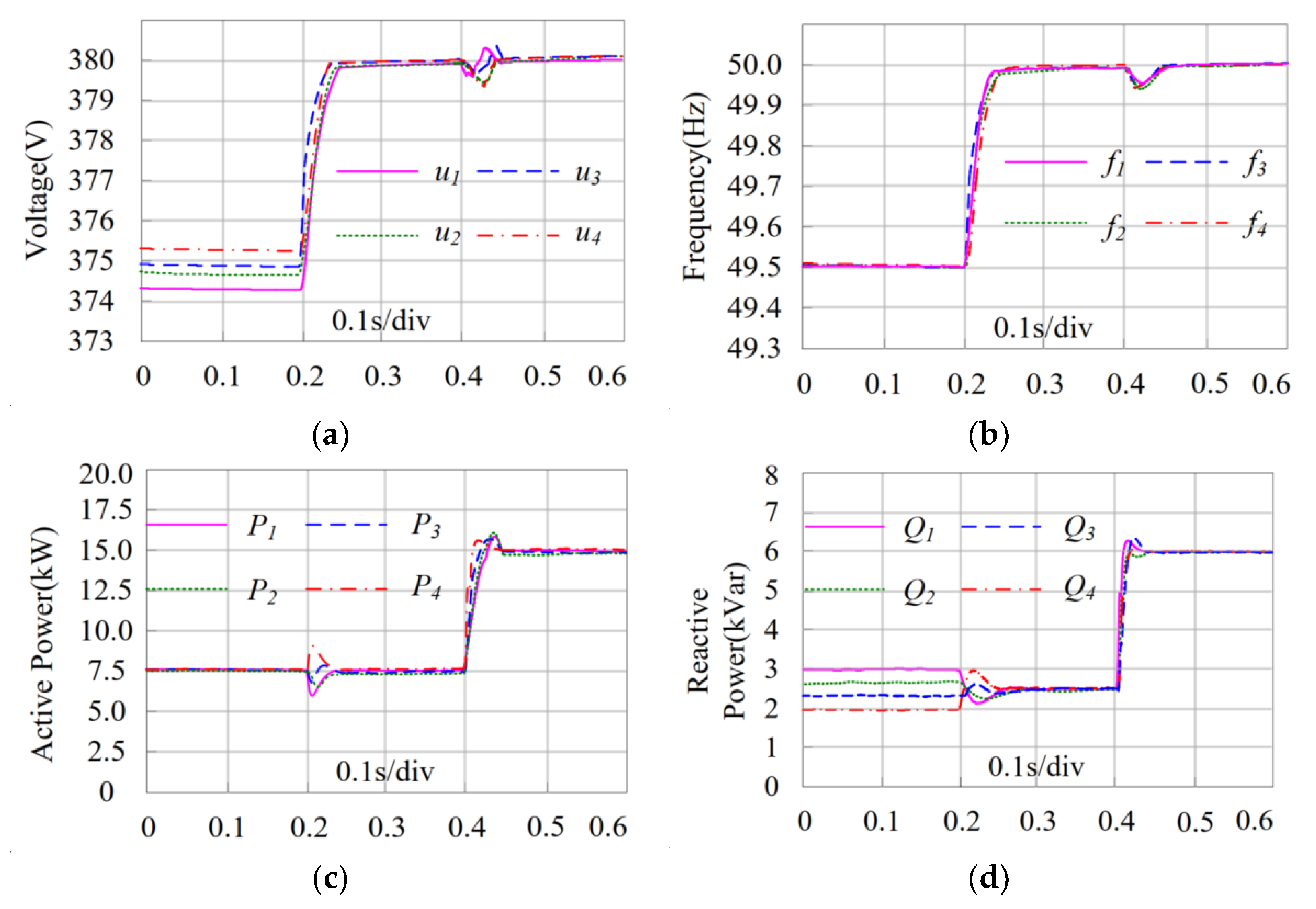
4.1. Case Study 1: Controller Performance

Figure 3 shows the distributed topology with four inverters and two loads.

The loads and lines are modeled as series RL branches. Among them, 1# inverter is the dominant node, which can directly obtain voltage and frequency reference value. Assuming that all inverters have the same capacity (25 kW, 10 kVar), the electrical parameters and simulation parameters of the system are shown in

Table 2. Electrical parameters.

Parameter	Value
R13, R24, R34	0.18 Ω, 0.28 Ω, 0.26 Ω
L13, L24, L34	0.26 mH, 0.28 mH, 0.16 mH
Load1	30 kW, 12 kVar
Load2	30 kW, 12 kVar

and

Table 3. Parameters of the proposed secondary controller.

Parameter	Value
mp, mq	2.68 × 10−5 rad/W, 0.9 × 10−3 V/Var
kω, kp	30, 40
m1, m2, m3	8, 16, 32
n1, n2, n3, n4	7, 5, 3, 5
Rref, Lref	0.06 Ω, 0.36 mH
kδ_L, kδ_R, kI	1.8 × 10−4, 1.06 × 10−2, 2.16

, respectively.

This case investigates the convergence performance of the proposed distributed control strategy. The simulation scenario is defined as follows, and the results are shown in Figure 4.

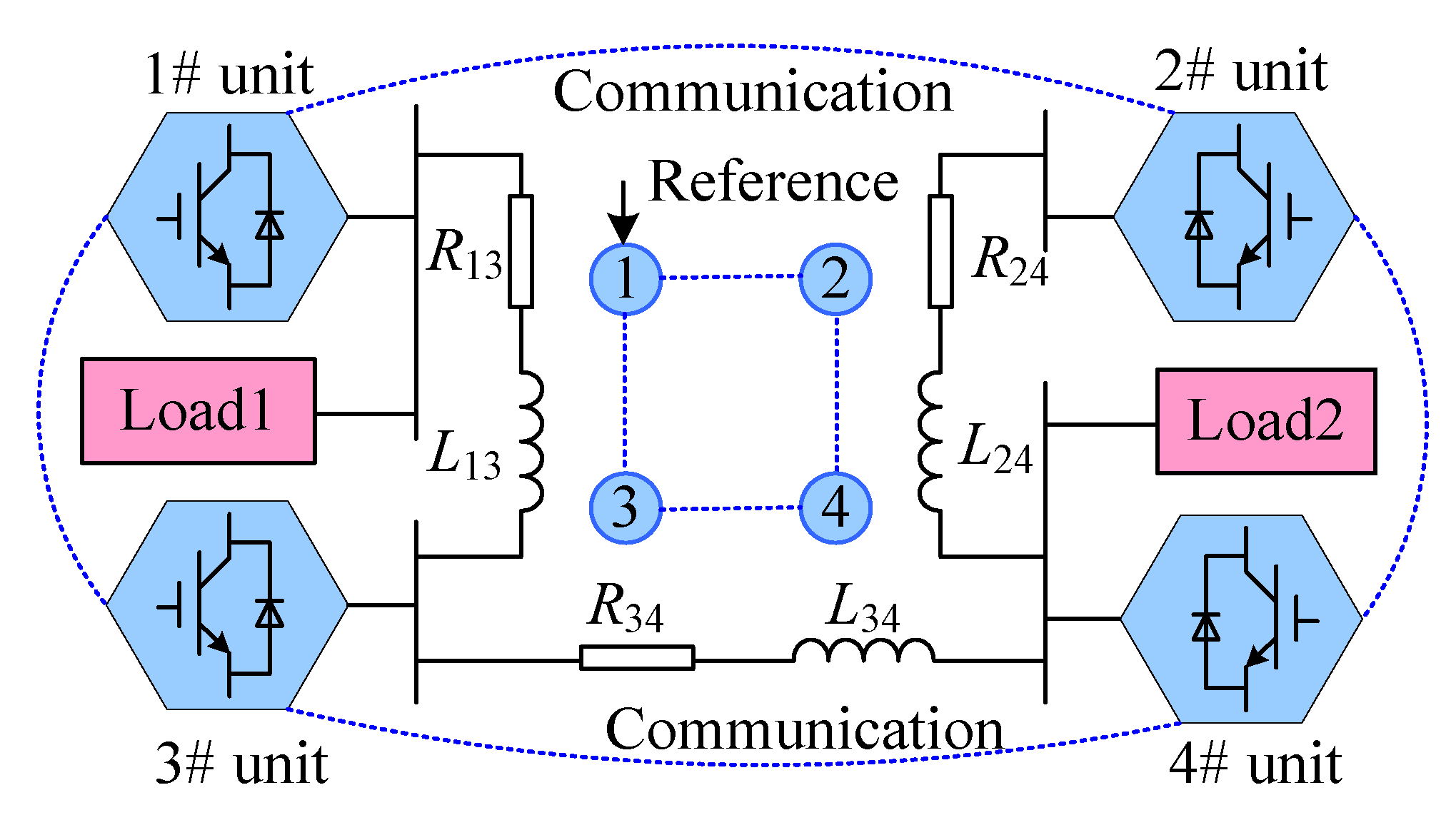
• t = 0.0 s (simulation initialization period), only the droop control is activated and only load#1 is connected to the network;
• t = 0.2 s, the proposed secondary control is applied;
• t = 0.4 s, Load#2 is connected.

During the period of 0–0.2 s, the voltage amplitudes of four units fall down to different values while the frequency can synchronize to a common value (49.5 Hz) by the droop control. The reactive power cannot be shared equally due to the mismatched line impedances either. Once the secondary controller is activated at stage 2, voltages of all units are restored to 380 V within 0.06 s, which validates the correctness of (50), since $T_v\le 0.0858$ and frequencies of all units are restored to 50 Hz within 0.05 s, which validates the correctness of (27), since $T_p\le 0.0778$. Therefore, the simulation results agree with the mathematical analysis. It is worth noting that, based on the distributed adaptive virtual impedance reactive power controller, the power sharing can also be satisfied. In the following, the load#2 is connected to the network at t = 0.4 s. The results show that the proposed distributed secondary controller shows good tracking and robust performance against the load connection. After small transient time, the voltages and frequency can be restored accurately, and the power sharing is still satisfied.

4.2. Case Study 2: Plug-and-Play Capability

In this study, the plug-and-play capability of the proposed secondary control strategy is tested by disconnecting 2# inverter from the system and reconnecting it to the network. Control parameters are selected in the same manner as in case study 1. Before the plug out of 2# inverter from the network, all inverters have already reached their steady state. The communication topology is also shown in Figure 2. This simulation study is divided into two stages, and the results are shown in Figure 5.

• At simulation in the initialization period (t = 0.0 s), the proposed secondary distributed controller is activated and t = 0.2 s, 2# inverter is disconnected from the network;
• At t = 0.4 s, 2# inverter is reconnected to the network.

As shown in Figure 5, once the 2# inverter is disconnected from the network at t = 0.2 s, its active and reactive power output will be reduced to zero, and the remaining inverters will provide more power to compensate for the power previously supplied by the 2# inverter. Due to the reactive power consistency controller, the power of the remaining inverters remains balanced.

At t = 0.4 s, when the 2# inverter is reconnected to the network, aside from some transients, the output power of the four inverters will still reach equilibrium, and the voltage amplitude and frequency will not deviate from its reference value. It can be seen from the results that, despite plug in and plug out operations of the 2# inverter, the proposed controllers maintain accurate power sharing and voltage and frequency restoration as well, which verify the ability of the proposed control method to satisfy the requirement of the plug-and-play operations.

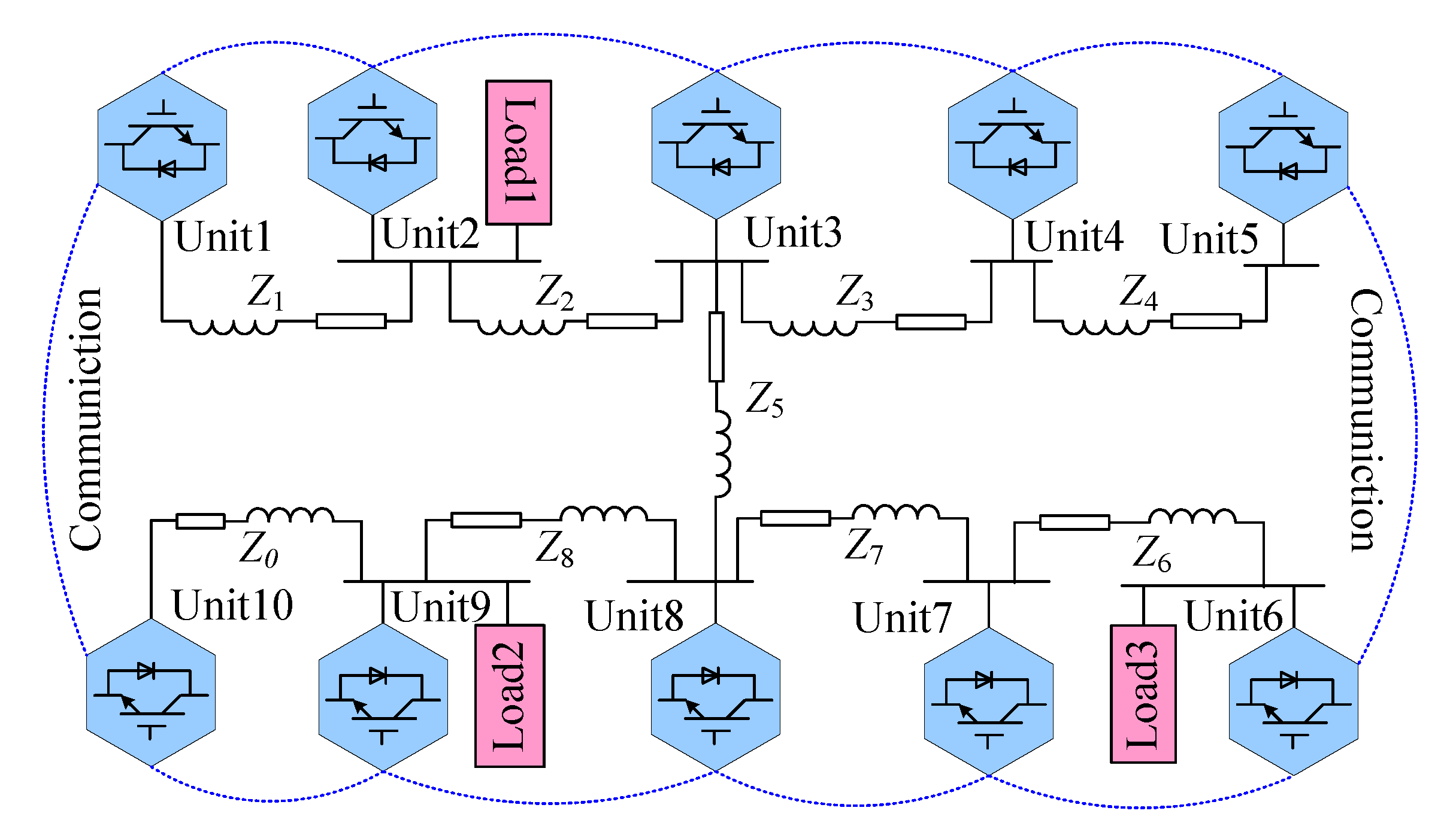
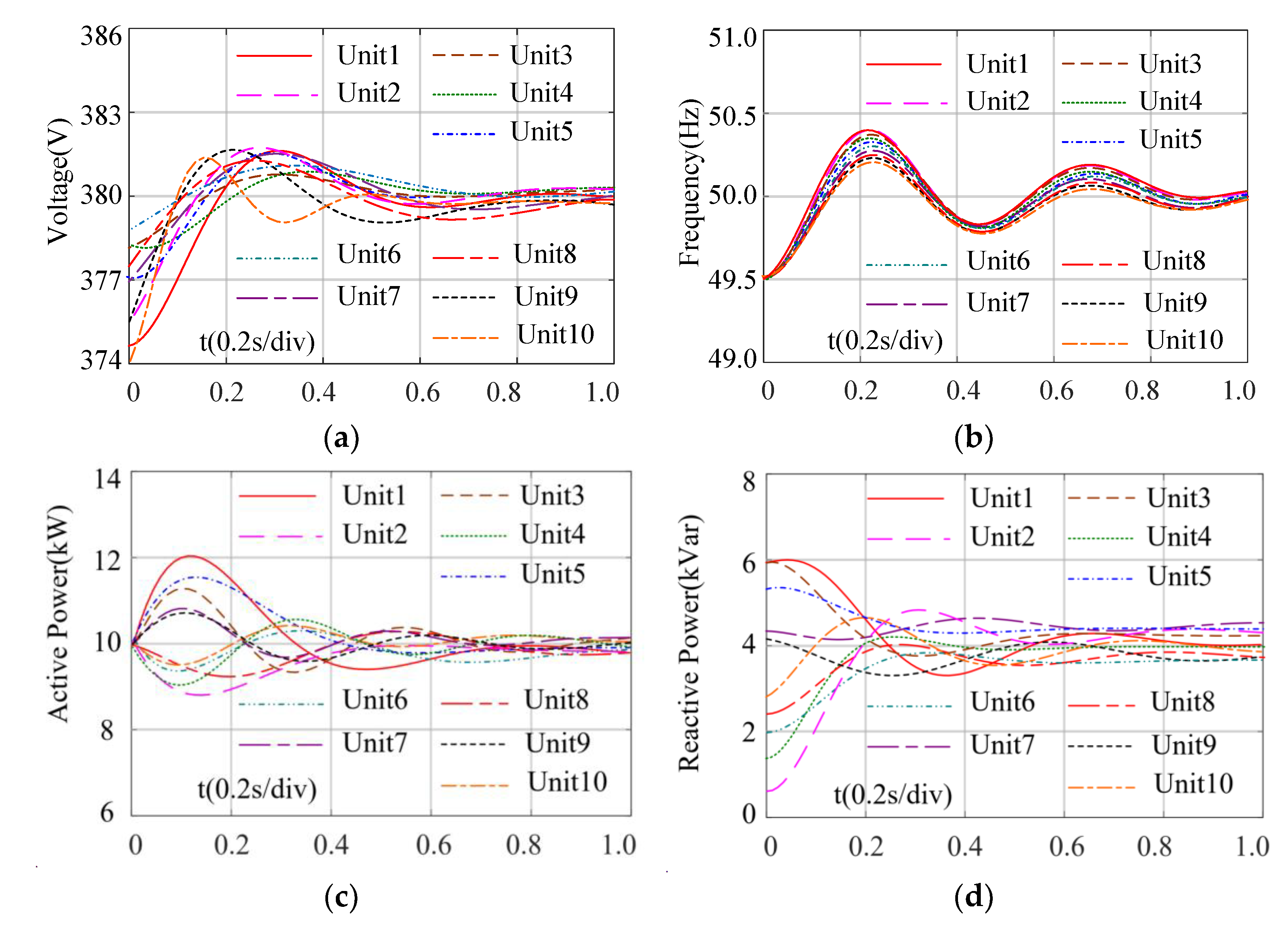
4.3. Case Study 3: Comparing the Proposed Method with Two Typical Methods in a Large System

As mentioned above, some research based on the distributed control protocol solves the voltage and frequency restoration issues, but these controllers are verified in a small-scale system consisting of four to five inverters. To better reflect the superiority of the proposed method, this paper compares the proposed controller with two typical distributed secondary controllers (the asymptotic controller proposed by [25] and the distributed finite-time controller proposed by [22]) in the large-scale system composed of 10 inverters shown in Figure 6.

The electrical parameters in the large-scale system are shown in

Table 4. The electrical parameters in a large system.

Parameter	Value
Z0, Z1, Z2	0.18 Ω, 0.26 mH
Z3, Z4, Z6	0.28 Ω, 0.28 mH
Z7, Z8, Z9	0.26 Ω, 0.16 mH
Z5	0.36 Ω, 0.36 mH
Load1	30 kW, 12 kVar
Load2	30 kW, 12 kVar
Load3	40 kW, 16 kVar

. For the sake of simplicity, it is assumed that the power levels of these 10 inverters are the same and the control parameters are shown as in Table 3.

According to the parameters in the references [22,25], the compared waveforms of frequency, voltage, and power are shown in Figure 7, Figure 8 and Figure 9. Note that the secondary controller is activated at t = 0 s, respectively. As shown in Figure 7, the restoration time under the linear consensus control algorithm in [25] is about 1.0 s. Although the controller guarantees the global asymptotic stability of the system, it has a longer convergence time and oscillation adjustment. Since the difference of line impedance is not considered, the reactive power sharing cannot be achieved. Compared with the algorithm in [25], the distributed finite-time controller in [22] can shorten the convergence time. As shown in Figure 8, the restoration time is about 500 ms. However, the controller protocol in [22] is established under a perfectly symmetric electrical network, the control parameters are very sensitive to system uncertainty. Therefore, there are still some fluctuations in the convergence process in this case. In addition, the reactive power sharing is not satisfied either. Under the proposed controller in this paper, using Equations (27) and (50), the estimated upper bounds of convergence time for frequency and voltage are 0.48 s and 0.38 s, respectively. As shown in Figure 9, the proposed control scheme enables the system to be restored to the references within the estimated upper bound. The convergence process is smoother. Compared to the control strategy in [22,25], the accurate reactive power distribution can be achieved.

To highlight the robust performance of the proposed controller, Figure 10, Figure 11 and Figure 12 show the compared simulation results with the above three algorithms under load change. Note at t = 0 s, load#3 is disconnected from the system. From the perspective of convergence time, the time under algorithm in [25] is the longest, reaching 0.88 s; the time under algorithm in [22] is 0.46 s, and the time under the proposed algorithm in this paper is the shortest, only about 0.3 s. From the perspective of power sharing, obvious mismatches among the reactive power of units are observed under algorithms in [22,25]. However, under the proposed algorithm in this paper, the reactive power sharing can be realized.

Figure 7, Figure 8, Figure 9, Figure 10, Figure 11 and Figure 12 verify the following results: (1) Compared to the algorithm in [22,25], the proposed control scheme can rapidly reach consensus, and show more robust performance for load change; (2) this control scheme can restore frequency and voltage to reference levels, and achieve active and reactive power sharing as well; and (3) this control scheme is independent of inverter parameters. By changing the connection structure of the communication link, the upper bound of convergence time can be reduced to some extent. Thus, the proposed control scheme is suitable for large-scale systems.

5. Conclusions

The problems of voltage and frequency restoration and power sharing are considered simultaneously in this paper. Compared with the centralized structure, in the proposed distributed controller, each unit is regarded as an agent of MAS, through the sparse communication network to realize the electrical information exchange between its neighbors. Therefore, the reliability, scalability, and flexibility can be greatly improved. In this paper, some knowledge about distributed consensus control theory is introduced firstly, and then the distributed finite-time approach is designed. In addition, to overcome the shortcoming of the mismatched load impedance influencing the reactive power sharing, the reactive power consistency control based on adaptive virtual impedance is proposed. At last, numerical simulations are carried out. Compared with the traditional methods, the results show the significant advantages of the proposed control scheme including robustness to load changes, plug-and-play capability, and improved convergence performance.

It should be noted that there are limitations to the proposed method, and some work should be done in the future. (1) For frequency restoration, the system initial state is the key factor to determine the upper bound of the convergence time. To get the accurate upper bound, it should be well estimated; (2) The distributed finite-time consensus problems for MAS with a virtual leader under the conditions of time-variant network topologies need further research; (3) In this paper, the communication graph is undirected and the communication networks do not suffer from any constrains. Directed communication graphs and the effect of communication delays on MAS also deserve investigation.

References

1. Meng, W.; Wang, X. Distributed Energy Management in Smart Grid With Wind Power and Temporally Coupled Constraints. IEEE Trans. Ind. Electron. 2017, 64, 6052–6062. [Google Scholar] [CrossRef]
2. Xu, Y.; Li, Z. Distributed Optimal Resource Management Based on the Consensus Algorithm in a Microgrid. IEEE Trans. Ind. Electron. 2015, 62, 2584–2592. [Google Scholar] [CrossRef]
3. Nunna, H.K.; Doolla, S. Multiagent-Based Distributed-Energy-Resource Management for Intelligent Microgrids. IEEE Trans. Ind. Electron. 2013, 60, 1678–1687. [Google Scholar] [CrossRef]
4. Olfati-Saber, R.; Murray, R.M. Consensus problems in networks of agents with switching topology and time-delays. IEEE Trans. Automat. Contr. 2004, 49, 1520–1533. [Google Scholar] [CrossRef] [Green Version]
5. Guerrero, J.M.; Vasquez, J.C.; Matas, J.; de Vicuna, L.G.; Castilla, M. Hierarchical Control of Droop-Controlled AC and DC Microgrids—A General Approach Toward Standardization. IEEE Trans. Ind. Electron. 2011, 58, 158–172. [Google Scholar] [CrossRef]
6. Espina, E.; Llanos, J.; Burgos-Mellado, C.; Cárdenas-Dobson, R.; Martínez-Gómez, M.; Sáez, D. Distributed control strategies for microgrids: An overview. IEEE Access. 2020, 8, 193412–193448. [Google Scholar] [CrossRef]
7. Prodanovic, M.; Green, T.C. High-Quality Power Generation Through Distributed Control of a Power Park Microgrid. IEEE Trans. Ind. Electron. 2006, 53, 1471–1482. [Google Scholar] [CrossRef] [Green Version]
8. Wang, L.; Xiao, F. Finite-time consensus problems for networks of dynamic agents. IEEE Trans. Automat. Contr. 2010, 55, 950–955. [Google Scholar] [CrossRef]
9. Yazdanian, M.; Mehrizi-Sani, A. Distributed Control Techniques in Microgrids. IEEE Trans. Smart Grid 2014, 5, 2901–2909. [Google Scholar] [CrossRef]
10. Cintuglu, M.H.; Youssef, T.; Mohammed, O.A. Development and application of a real-time testbed for multiagent system interoperability: A case study on hierarchical microgrid control. IEEE Trans. Smart Grid 2018, 9, 1759–1768. [Google Scholar] [CrossRef]
11. Morstyn, T.; Hredzak, B.; Agelidis, V.G. Control Strategies for Microgrids with Distributed Energy Storage Systems: An Overview. IEEE Trans. Smart Grid 2018, 9, 3652–3666. [Google Scholar] [CrossRef] [Green Version]
12. Shafiee, Q.; Guerrero, J.M.; Vasquez, J.C. Distributed secondary control for islanded microgrids-a novel approach. IEEE Trans. Power Electron 2014, 29, 1018–1031. [Google Scholar] [CrossRef] [Green Version]
13. Zhang, H.; Kim, S.; Sun, Q.; Zhou, J. Distributed Adaptive Virtual Impedance Control for Accurate Reactive Power Sharing Based on Consensus Control in Microgrids. IEEE Trans. Smart Grid 2017, 8, 1749–1761. [Google Scholar] [CrossRef]
14. Shafiee, Q.; Nasirian, V.; Vasquez, J.C.; Guerrero, J.M.; Davoudi, A. A Multi-Functional Fully Distributed Control Framework for AC Microgrids. IEEE Trans. Smart Grid 2018, 9, 3247–3258. [Google Scholar] [CrossRef] [Green Version]
15. Hu, J.; Duan, J.; Ma, H.; Chow, M.Y. Distributed Adaptive Droop Control for Optimal Power Dispatch in DC Microgrid. IEEE Trans. Ind. Electron. 2018, 65, 778–789. [Google Scholar] [CrossRef]
16. Lu, X.; Yu, X.; Lai, J.; Guerrero, J.M.; Zhou, H. Distributed Secondary Voltage and Frequency Control for Islanded Microgrids With Uncertain Communication Links. IEEE Trans. Ind. Inform. 2017, 13, 448–460. [Google Scholar] [CrossRef] [Green Version]
17. Deng, Z.; Xu, Y.; Sun, H.; Shen, X. Distributed, Bounded and Finite-Time Convergence Secondary Frequency Control in an Autonomous Microgrid. IEEE Trans. Smart Grid 2019, 10, 2776–2788. [Google Scholar] [CrossRef]
18. Guan, Z.H.; Sun, F.L.; Wang, Y.W.; Li, T. Finite-Time Consensus for Leader-Following Second-Order Multi-Agent Networks. IEEE Trans. Circuits Syst. I Regul. Pap. 2012, 59, 2646–2654. [Google Scholar] [CrossRef]
19. Lu, X.; Lu, R.; Chen, S.; Lu, J. Finite-time distributed tracking control for multi-agent systems with a virtual leader. IEEE Trans. Circuits Syst. I Regul. Pap. 2013, 60, 352–362. [Google Scholar] [CrossRef]
20. Lou, G.; Gu, W.; Xu, Y.; Cheng, M.; Liu, W. Distributed MPC-Based Secondary Voltage Control Scheme for Autonomous Droop-Controlled Microgrids. IEEE Trans. Sustain. Energy 2017, 8, 792–804. [Google Scholar] [CrossRef]
21. Guo, F.; Wen, C.; Mao, J.; Song, Y.D. Distributed Secondary Voltage and Frequency Restoration Control of Droop-Controlled Inverter-Based Microgrids. IEEE Trans. Ind. Electron. 2015, 62, 4355–4364. [Google Scholar] [CrossRef]
22. Zuo, S.; Davoudi, A.; Song, Y.; Lewis, F.L. Distributed Finite-Time Voltage and Frequency Restoration in Islanded AC Microgrids. IEEE Trans. Ind. Electron. 2016, 10, 5988–5997. [Google Scholar] [CrossRef]
23. Lai, J.; Lu, X.; Xin, L.; Tang, R.L. Distributed Multiagent-oriented Average Control for Voltage Restoration and Reactive Power Sharing of Autonomous Microgrids. IEEE Access. 2018, 6, 25551–25561. [Google Scholar] [CrossRef]
24. Xu, Y.; Sun, H. Distributed Finite-Time Convergence Control of an Islanded Low-Voltage AC Microgrid. IEEE Trans. Power Syst. 2018, 33, 2339–2348. [Google Scholar] [CrossRef]
25. Bidram, A.; Member, S.; Davoudi, A.; Lewis, F.L.; Guerrero, J.M.; Member, S. Distributed Cooperative Secondary Control of Microgrids Using Feedback Linearization. IEEE Trans. Power Syst. 2013, 28, 3462–3470. [Google Scholar] [CrossRef] [Green Version]
26. Bidram, A.; Davoudi, A.; Lewis, F.L.; Qu, Z. Secondary control of microgrids based on distributed cooperative control of multi-agent systems. IET Gener. Transm. Distrib. 2013, 7, 822–831. [Google Scholar] [CrossRef] [Green Version]
27. Bhat, S.P.; Bernstein, D.S. Finite-time stability of continuous autonomous systems. SIAM J. Control Optim. 2000, 38, 751–766. [Google Scholar] [CrossRef]
28. Simpson-Porco, J.W.; Shafiee, Q.; Dorfler, F.; Vasquez, J.C.; Guerrero, J.M.; Bullo, F. Secondary Frequency and Voltage Control of Islanded Microgrids via Distributed Averaging. IEEE Trans. Ind. Electron. 2015, 62, 7025–7038. [Google Scholar] [CrossRef]
29. Han, H.; Liu, Y.; Sun, Y.; Su, M.; Guerrero, J.M. An Improved Droop Control Strategy for Reactive Power Sharing in Islanded Microgrid. IEEE Trans. Power Electron. 2014, 30, 3133–3141. [Google Scholar] [CrossRef] [Green Version]
30. Li, Y.W.; Kao, C.N. An accurate power control strategy for power-electronics-interfaced distributed generation units operating in a low-voltage multibus microgrid. IEEE Trans. Power Electron. 2009, 24, 2977–2988. [Google Scholar]
Figure 1. The control diagram of an islanded inverter-based DG.
Energies 14 06266 g001
Figure 2. Block diagram of the distributed finite-time secondary control.
Energies 14 06266 g002
Figure 3. Simulation test setup.
Energies 14 06266 g003
Figure 4. The simulation performance of case study 1. (a) Voltage amplitude; (b) Frequency; (c) Active power; (d) Reactive power.
Energies 14 06266 g004
Figure 5. The simulation performance of case study 2. (a) voltage amplitude; (b) frequency; (c) active power; (d) reactive power.
Energies 14 06266 g005
Figure 6. The large system with ten inverters.
Energies 14 06266 g006
Figure 7. The simulation results with the control strategy in [25]. (a) voltage amplitude; (b) frequency; (c) active power; (d) reactive power.
Energies 14 06266 g007
Figure 8. The simulation waveforms with the control strategy in [22]. (a) voltage amplitude; (b) frequency; (c) active power; (d) reactive power.
Energies 14 06266 g008
Figure 9. The simulation results with the proposed control strategy in this paper. (a) voltage amplitude; (b) frequency; (c) active power; (d) reactive power.
Energies 14 06266 g009
Figure 10. The simulation results with the control strategy in [25] under load change at t = 0 s. (a) voltage amplitude; (b) frequency; (c) active power; (d) reactive power.
Energies 14 06266 g010aEnergies 14 06266 g010b
Figure 11. The simulation results with the control strategy in [22] under load change at t = 0 s. (a) voltage amplitude; (b) frequency; (c) active power; (d) reactive power.
Energies 14 06266 g011
Figure 12. The simulation waveforms with the proposed control strategy under load change at t = 0 s. (a) voltage amplitude; (b) frequency; (c) active power; (d) reactive power.
Energies 14 06266 g012aEnergies 14 06266 g012b