Forecasting Natural Gas Production and Consumption in United States-Evidence from SARIMA and SARIMAX Models

Abstract

Research on forecasting the seasonality and growth trend of natural gas (NG) production and consumption will help organize an analysis base for NG inspection and development, social issues, and allow industrials elements to operate effectively and reduce economic issues. In this situation, we handle a comparison structure on the application of different models in monthly NG production and consumption forecasting using the cross-correlation function and then analyze the association between exogenous variables. Moreover, the SARIMA-X model is tested for US monthly NG production and consumption prediction via the proposed method for the first time in the literature review in this study. The performance of that model has been compared with SARIMA (p, d, q) * (P, D, Q)^s. The results from RMSE and MAPE indicate that the superiority of the best model. By applying this method, the US monthly NG production and consumption is forecast until 2025. The success of the proposed method allows the use of seasonality patterns. If this seasonal approach continues, the United States’ NG production (16%) and consumption (24%) are expected to increase by 2025. The results of this study provide effective information for decision-makers on NG production and consumption to be credible and to determine energy planning and future sustainable energy policies.

1. Introduction

Global warming has a critical problem in countries all over the world, seriously threatening the development and survival of human beings especially in recent years. However, most countries have started to explore clean and low-greenhouse gas energy transitions and are beginning to decrease greenhouse gas emissions [1]. Likewise, most countries have improved a transition in the energy matrix to reduce greenhouse gas emissions without restricting economic growth [2] and environmental politics [3]. An energy outlook report has forecast that the global demand for natural gas will increase in the next 15 years [4]. The comparison of petroleum and coal, natural gas blaze absolutely, and remainder content were minimized. Therefore, it purposes low emission more than fossil fuels [5]. Moreover, both liquefied petroleum gas and natural gas could act as intermediate fuels to control environmental pollution [6].

Natural gas (NG) is the only non-renewable energy resource [7], and the most applied energy resource in certain societies [8]. Its dependency is increasing day by day in oil and gas developed countries [9,10,11,12]. However, according to the 2020 statistics energy review report by British Petroleum, natural gas production has increased by 132 (bcm) or 3.4%, and natural gas consumption has increased by 78 (bcm) or 2%, one of the strongest growth rates seen in 2018 [13].

Energy management is the most challenging issue as today’s situation will greatly affect future outcomes. Managing energy sources is the most important duty of decision-makers and lawmakers [14], along with policymakers and other stakeholders [11]. Moreover, energy management is the main concern in preparing energy policy for developing countries [15]. The most used energy management variables are natural gas, all of which are imported. Evaluating natural gas consumption such as annually, monthly, weekly, daily, and hourly, will lead to the management of plans such as transportation, distribution, and natural gas production [16,17], along with sampling frequency, such as yearly, daily, and hourly [18,19]. In daily studies, NG demand was predicted. A successful daily NG forecasting will lead to determining temperature, pipeline pressures, the viscosity of the gas [8,20], and exogenous variables [21].

Furthermore, advantages in evaluating NG consumption in the short term can include “Sales agreements and supply of gas” [22]. The layout of the reference pipelines and gas storage facility development empowers a more capable NG network optimization [23,24], and NG transmission network [25]. This ensures that supply and supply are in balance [8,18]. An advantageous short-term NG prediction estimation contributes to social contributions [1,25]. It grants industrial chain components to the event effectively with minimal economic loss [26,27]. The existing literature tending to the individual financial and commodity markets has significantly shifted through the recent global pandemic [28].

In recent years, different NG production and consumption prediction methods have been continuously applied. These forecasting methods can be divided into: time series methods and machine learning methods. Linear regression and time series-based models analyze the association between the ‘output variable’ and exogenous factors; commonly, the relationship is indicated linearly. This model is applied for NG forecasting [26]. Though linear regression models are surely applicable, they prove a weakness in indicating “non-linear” relationships. It is insufficient to interpret via a non-linear and linear relationship such as NG consumption [29]. Time-series methods can be determined as natural relationships. They are widely used in natural gas consumption forecasts [10,30,31,32,33,34]. Although machine learning models can be determined, their relationships are usually non-natural. They are widely applied in evaluating natural gas consumption [35,36,37]. Furthermore, NG production and consumption forecasts are necessary for the sustainable growth of all countries.

In this study, according to the available statistics report, the production and consumption for NG will increase in future years equal to the increasing growth of the United States. Studies of the production and consumption forecast in the review of the literature are performed yearly. Although, the aim of seasonal production and consumption for NG cannot be expected through annual studies. For this reason, this study focuses on the United States natural gas production and consumption forecasted monthly by focusing on the seasonal balance, natural gas supply/demand, peak shaving, residential, commercial, transportation, and industrial. For correlation between monthly production and consumption forecast, the more accurate SARIMAX (p, d, q) * (P, D, Q)^s forecasting model was proposed as a new approach. This is the first used in the field of natural gas. To show the performance of the models, the basic SARIMA (p, d, q) * (P, D, Q)^s model—a popular technique—is performed, and two methods have been compared with forecast success. Therefore, correlativity between the monthly NG production and consumption and seasonal exogenous variables was reliably predicted by SARIMAX (p, d, q) * (P, D, Q)^s model to determine high forecast success. Finding the right model based on natural gas data is part of our contributions. Based on these exogenous factors, the superiority in order accuracy was achieved.

2. Material and Methods

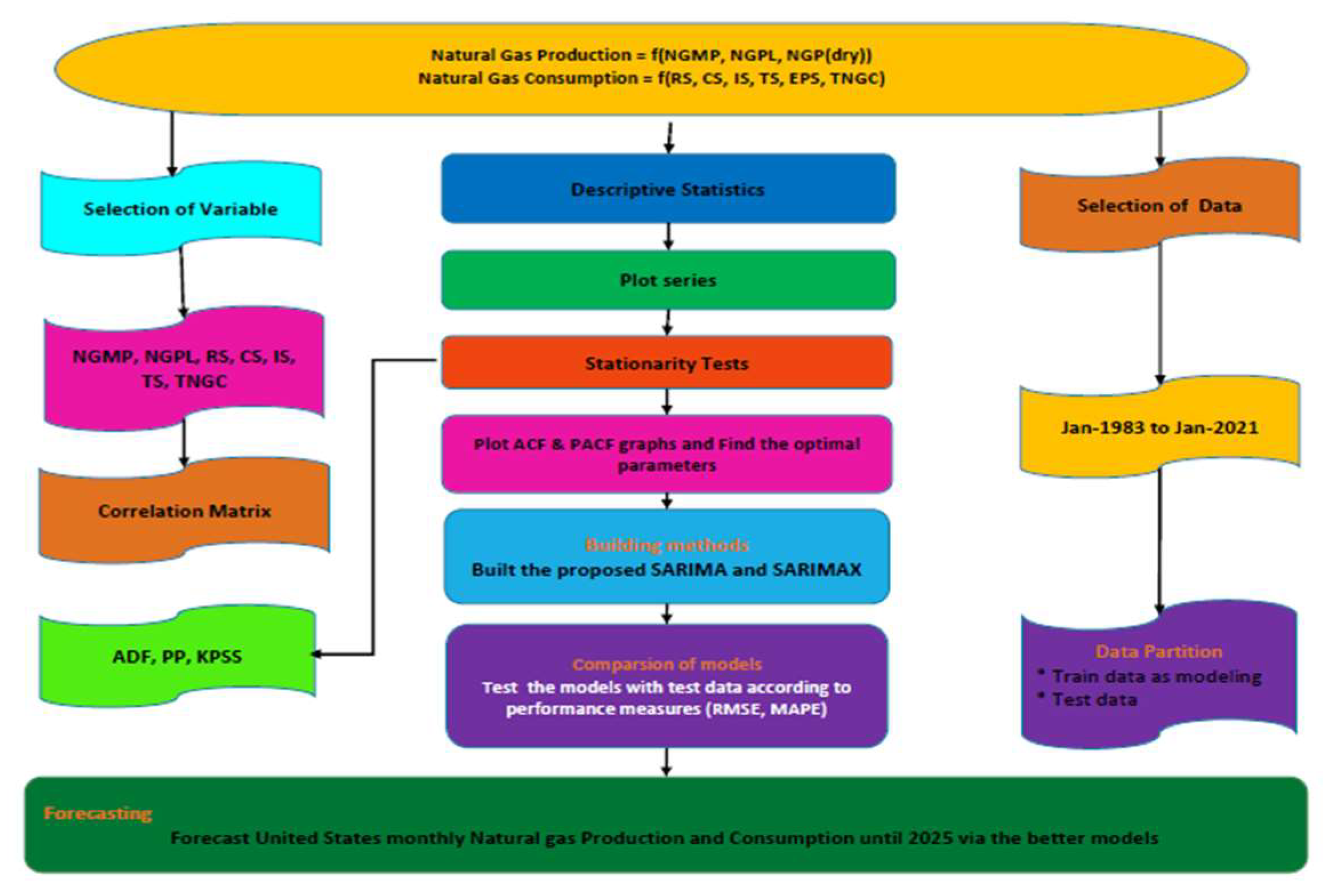
Natural gas production and consumption of the United States (US) is forecast until 2025 on a monthly basis. For this study, a system process in the collection of data and dataset partitions, models building, comparative analysis of the models, prediction, and estimations steps are followed. The research flowchart is indicated in Figure 1.

Figure 1. Research flowchart.

2.1. Data Measurement

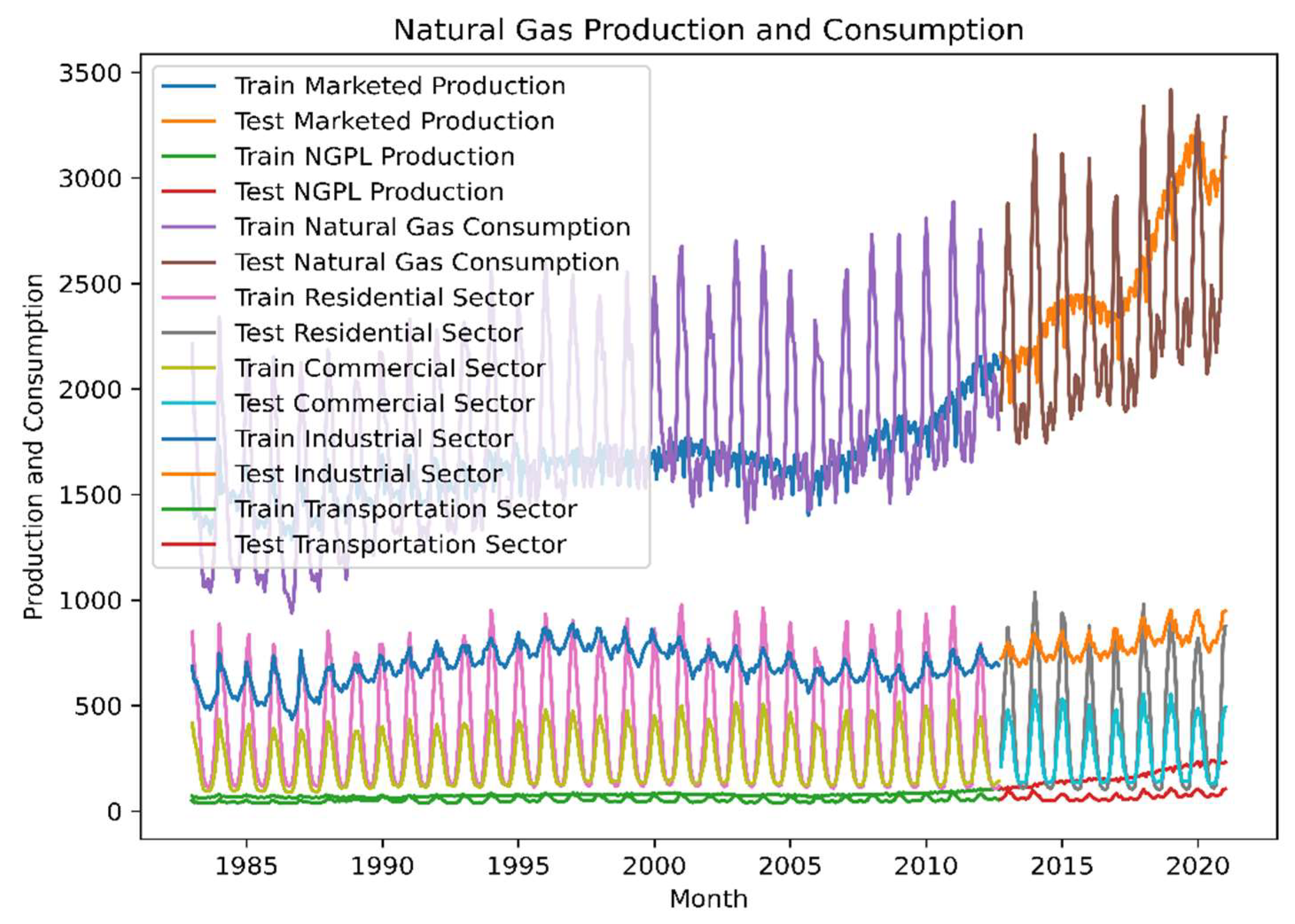
United States natural gas data was taken from the Energy Information Administration. Then, we selected the variables—natural gas production and consumption (NGP and NGC). This information contains monthly natural gas and renewal energy between January 1983 to January 2021. The dataset is shown graphically in Figure 2. It indicates that the dataset is seasonal with a growth trend. The dataset was divided into training and test sets. The last 40 seasonal years in the training sets is used to organize an identical estimation of SARIMAX (p, d, q) * (P, D, Q)^s models.

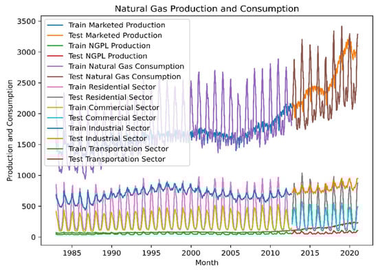
Figure 2. US natural gas production and consumption factors between January 1983 to January 2021.

2.2. Methods for Time Series Analysis

2.2.1. ARIMA and ARIMAX Methods

The Box–Jenkins model was used (Box et al. 1994). The ARIMA model is considered to be the future values of a linear function with past values and random errors [38]. One of the most common methods used in the time series analysis is the ARIMA model. The ARIMA model consists of the terms autoregressive model (AR), integration (I), and moving average (MA) [39]. ARIMAX proposed the model by expanding the ARIMA model [40]. In this method, extra independent variables are applied in addition to the ARIMA method. The ARIMAX method can be specified as follows [41]:

$$\begin{gathered} y_t=\alpha +{\displaystyle \sum _{i=1}^m\frac{{\gamma }_i\left(G\right)}{{\phi }_i\left(G\right)}}Gl{X}^{it}+e_t \\ \therefore e_t=\frac{\gamma \left(G\right)}{\phi \left(G\right)}{a}_t \end{gathered}$$

(1)

where $\phi \left(G\right)$ denotes the AR coefficients, $\gamma \left(G\right)$ presents the MA coefficients, $l_i$ indicates the degree of lag, $e_t$ shows the error analysis in regression, $a_t$ Zero average with error terms time series.

2.2.2. SARIMA Models

The seasonal ARIMA (p, d, q) * (P, D, Q)^s model is a development of ARIMA which was introduced to advance the performance of auto-regressive integrated moving average in modeling the seasonal series [42,43,44,45]. The general form [46,47] of the seasonal ARIMA method is expressed as given in the following Equation (2):

$${\phi }_p\left(G\right){\varphi }_P\left(G^{seasonal}\right){\left(1-G\right)}^d{\left(1-G^{seasonal}\right)}^D{X}_t={\gamma }_q\left(G\right){\omega }_Q\left(G^{seasonal}\right)e_t$$

(2)

Expression ${\phi }_p\left(G\right)$ and ${\gamma }_q\left(G\right)$ indicate the order of the characteristic polynomial of non-seasonal autoregressive (AR) and non-seasonal moving average (MA) components. The terms ${\varphi }_P\left(G^{seasonal}\right)$ ${\omega }_Q\left(G^{seasonal}\right)$ and indicate the seasonal autoregressive (SAR) and seasonal moving average (SMA) polynomial. $\left(1-G\right)$ and $\left(1-G^{seasonal}\right)$ indicates the non-seasonal and seasonal time series are differencing components, respectively. The terms are d and D indicate the ordinary differenced terms of non-seasonal ARIMA, seasonal differenced terms of the seasonal ARIMA of the series [48,49]. In addition, $X_t$ indicates the observed value at the time $t$, $e_t$ stands for error terms of prediction, and $s$ is the length of the seasonal pattern (e.g., s = 12, monthly series) and $G$ is the backshift operator terms, respectively.

The SARIMA components can be written as follows:

• AR: ${\phi }_p\left(G\right)=1-{\phi }_{1}G-{\phi }_2{G}^2-{\phi }_3{G}^3-\cdots -{\phi }_p{G}^p$,
• MA: ${\gamma }_q\left(G\right)=1-{\gamma }_{1}G-{\gamma }_2{G}^2-{\gamma }_3{G}^3-\cdots -{\gamma }_q{G}^{{}_q}$,
• SAR: ${\varphi }_P\left(G^{seasonal}\right)=1-{\varphi }_1{G}^{seasonal}-{\varphi }_2{G}^2{}^{seasonal}-{\varphi }_3{G}^3{}^{seasonal}-\cdots -{\phi }_P{G}^P{}^{seasonal}$,
• SMA: ${\omega }_Q\left(G^{seasonal}\right)=1-{\omega }_1{G}^{seasonal}-{\omega }_2{G}^2{}^{seasonal}-{\omega }_3{G}^3{}^{seasonal}-\cdots -{\omega }_Q{G}^Q{}^{seasonal}$.

2.2.3. Seasonal ARIMA with eXogenous Factors (SARIMAX)

Seasonal ARIMAX is an advancement of the seasonal ARIMA with external feature variables (X) called SARIMAX $\left(p,d,q\right)\ast \left(P,D,Q\right)$, to improve its prediction and performance. The seasonal ARIMAX model can be suggested as follows [50];

$${\phi }_p\left(G\right){\varphi }_P\left(G^{seasonal}\right){\left(1-G\right)}^d{\left(1-G^{seasonal}\right)}^D{X}_t={\alpha }_k{y}_{k,t}+{\gamma }_q\left(G\right){\omega }_Q\left(G^{seasonal}\right)e_t$$

(3)

where $y_{k,t}$ are the corresponding observations of the $k^{th}$ represented as the number of exogenous variables at the time $t$, and ${\alpha }_k$ represents the correlation coefficient value of the $k^{th}$ exogenous (X) input variables.

The seasonal ARIMA model with exogenous factors develops the capacity of the seasonal ARIMA model by integration of contextual information such as air temperature, humidity, average cold cover, wind speed, and other meteorological variables that affect natural gas demand and consumption [32]. Similarly, the indoor pollutant CO2 [51], mumps cases [52], and scarlet fever [53] were found in a study in the literature. In the current study, the SARIMAX method was organized to investigate natural gas production and consumption. The determining methods used to produce the model are given below.

Step 1: The data of time series is integration determines the order d(1,2) stationery.

Step 2: The selection of order AR and MA in the model parameters are determined for use in seasonal and non-seasonal ACF and PACF diagrams using determined values of (p, d, q) * (P, D, Q)^s parameters estimated for the SARIMA and SARIMAX models. We assessed the relationship between pair sequences with robust autocorrelation. The cross-correlation function diagram was used to estimate the association between the NGP, NGC, and exogenous variables—also determined with covariates and lags selected for the best model. The Akaike information criterion and Schwarz Bayesian criterion values were used to assess the performance of the best model fit. Minimal AIC and BIC values indicate the best model fitting [54].

2.3. Analysis and Measures of Performance

To evaluate, the measure used to forecast the models in this study is the root mean square error (RMSE) and mean absolute percentage error (MAPE) [55,56,57], (Barnston 1992) shown in Equations (4) and (5), given below;

$$\mathrm{MAPE}\%=\frac{{\displaystyle \sum _{t=1}^n\frac{\left|E_t-F_t\right|}{E_t}}}{n}$$

(4)

$$\mathrm{RMSE}=\sqrt{\frac{1}{n}{\displaystyle \sum _{t=1}^n{\left(E_t-F_t\right)}^2}}$$

(5)

where $\left(E_t\right)$ and $\left(F_t\right)$ represents the actual values and forecast values at $t$ the time respectively, $n$ is the estimate values.

3. Experimental Results and Discussion

Table 1 presents summary statistics of natural gas production and consumption between January 1983 to January 2021. The US have maximally natural gas consumption at 3417.27, therefore, its minimum natural gas production is 3232.45. The maximal values for the natural gas market production and NGPL production are 3232.45 and 240.70, respectively. Similarly, residential, commercial, industrial, transport, and total natural gas consumption is 1037.19, 571.74, 952.25, 109.53, and 3417.27, respectively. Moreover, the minimal natural gas market production and NGPL production are 1284.80 and 59.96, respectively. Similarly, residential, commercial, industrial, transport, and total natural gas consumption is 99.78, 88.74, 435.47, 36.30, and 939.93, respectively. Looking at the standard deviation, natural gas consumption is more than natural gas production. Superior and inferior kurtosis can be found in natural gas production variables and natural gas consumption variables, which ensures the presence of a fat tail distribution. The natural gas production and consumption are almost positively skewed as the small p-values of the JB (Jarque–Bera test) reject the normality of the null hypothesis.

Table 1. Statistical summary of descriptions for natural gas production and consumption.

Metrics	N	Mean	Std.	Min.	Max.	Skew.	Kurt.	J–B Test	p-Values
Natural Gas Production
Market Prod.	457	1832.86	435.047	1284.80	3232.45	1.488	1.464	206.811	0.0 **
NGPL	457	95.536	41.620	59.96	240.70	1.921	2.813	425.434	0.0 **
Natural Gas Consumption
Total NGC	457	1894.5	486.52	939.93	3417.27	0.538	0.014	21.97	0.000 ***
Residential	457	393.66	271.319	99.78	1037.19	0.565	−1.11	48.0025	0.000 ***
Commercial	457	248.82	125.95	88.74	571.74	0.603	−0.97	45.877	0.000 ***
Industrial	457	709.57	94.09	435.47	952.25	−0.19	0.031	2.822	0.243
Transport	457	56.53	14.63	36.30	109.53	0.957	0.522	74.20	0.000 ***

Authors compilation; This table shows that the include minimum, maximum, mean, standard deviation, kurtosis, and skewness measure (descriptive statistics) for the monthly dataset used in this studies for the natural gas production sector and consumption sector defined in this work. All the series in the table are in actual terms: natural gas production and consumption. JB refers to the statistic of the Jarque-Bera (JB) test normality (p > 0.05 presented the normality of series). Asterisk ***,** represents statistical significance at the 1% and 5% level, accordingly.

3.1. The Findings of the ADF, KPSS, and PP Unit Root Tests

The preliminary steps needed for time series methods is the inquiry of the integration of order into all variables. In the present study, we have used unit root tests, which are [58], ADF [59,60], and KPSS [61], and PP test [62,63] to extract information concerning the integration of order, and the unit root results are shown in Table 2. The unit root tests results suggest that all variables are non-stationarity by level form; however, we first-order differenced [i.e., I(1)] them to make them stationary with Market Production, NGPL, Total NGC, Residential, Commercial, Industrial, and Transport been series are stationary statistical significance at 1%, 5%, and 10% levels. All stationary as represented by the ADF, KPSS, and PP test results.

Table 2. Summary of unit root tests.

Variable	ADF-Test		PP-Test		KPSS-Test
	Level	1st Order	Level	1st Order	Level	1st Order
Natural Gas Production
Market Prod.	0.7100	−4.102 ***	0.195	−53.844 ***	1.865	0.5488 *
NGPL	1.831	−2.767 **	3.502	−41.762 ***	1.624	1.1038 *
Natural Gas Consumption
Total NGC	−0.020	−7.638 ***	−5.700	−13.675 ***	2.083	0.076 **
Residential	−4.294 ***	−8.594 ***	−5.300 ***	−7.718 ***	0.036	0.0451 **
Commercial	−2.350	−8.050 ***	−5.305	−7.743 ***	0.892	0.042 **
Industrial	−1.366	−5.915 ***	−3.971	−27.580 ***	0.875	0.087 **
Transport	−0.712	−6.064 ***	−5.397	−14.635 ***	1.526	0.068 **

Author's compilation; ADF, KPSS, and PP tests are performed where *, **, and *** indicate that the null hypothesis is rejected at 1%, 5%, and 10% levels, respectively.

3.2. Correlation Coefficient Matrix

The correlation coefficient matrix is shown in Table 3. There is a statistically significant positive correlation between Natural gas production and NG consumption. The correlation coefficient between market production and NGPL production in the United States is 0.979771; in the commercial sector and residential sector with superior consumption growth, it is 0.985891, and total Natural gas consumption and transportation sector is 0.931583, the results are presented in Table 3.

Table 3. Correlation matrix results.

Natural Gas Production
Variables	Marketed Production		NGPL
Market Prod.	1		-
NGPL	0.979771 ***		1
Natural Gas Consumption
Variables	Residential	Commercial	Industrial	Transportation	Total NGC
Residential	1	-	-	-	-
Commercial	0.985891 ***	1	-	-	-
Industrial	0.459358	0.554703	1	-	-
Transportation	0.701081	0.775182	0.764186	1	-
Total NGC	0.756160	0.837779	0.776586	0.931583 ***	1

Authors compilation; Asterisk *** represents statistical significance at the 1% level, accordingly.

3.3. Application of SARIMA and SARIMAX Models on Natural Gas Production and Consumption

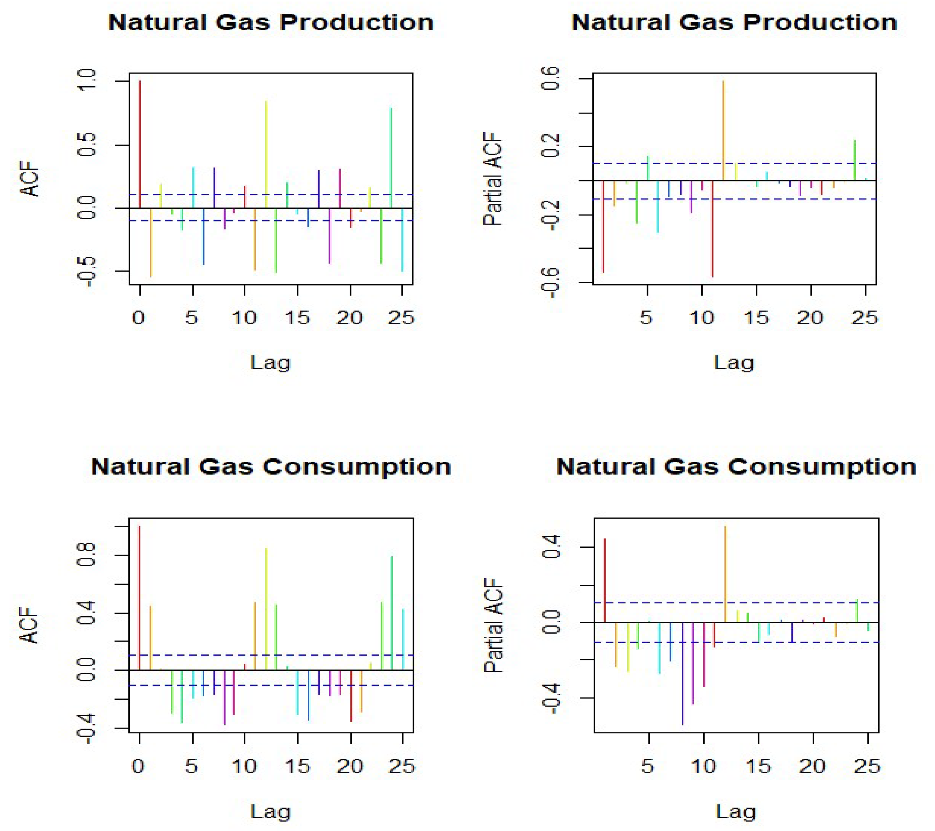
The proposed SARIMA and SARIMAX (X is exogenous variables) time-series methods are advanced for the monthly series of natural gas production and consumption with other exogenous factors (production sector and consumption sector). The ADF [59,60], KPSS [61], and PP [62,63] unit root tests for the series natural gas production and consumption data are tests for stationary (reported in Table 2). In the series of the monthly data after the first order integration process and seasonal integration, values of both D and d are 1. The ACF and PACF graphic of the natural gas production sector and consumption sector are presented in Figure 3. The autocorrelation function of lag values exceeds the critical values in the natural gas production and consumption sector. In the ACF of lag, values such as natural gas production and consumption sectors are cross-effective of the non-seasonal and seasonal autocorrelation. Moreover, the appropriate maximal values of the non-seasonal criteria (Q) and the seasonal criteria (q) are 1 and 2. Furthermore, the sample PACF values of lag that are significant are natural gas production and consumption sectors (Figure 3), so the appropriate maximal values of the non-seasonal criteria (p) and the seasonal criteria (P) are 2 and 4. Table 4 presents the best fit model based on significant parameters and coefficient statistics. The p-values are always p > 0.05, this model's criteria estimation appears statistically significant in the appropriate structure of seasonal ARIMA. The best-fitted model is NG production SARIMA (4,1,1) * (1,0,1)¹² and consumption SARIMA (2,1,1) * (5,0,0)¹². Accordingly, the selected lowest values of AIC and BIC are presented in Table 4. The sufficiency of the seasonal ARIMA (4,1,1) * (1,0,1)¹² and SARIMA (2,1,1) * (5,0,0)¹² model is verified by the LB (Q) test statistics (0.01) for which the p-values (Production 0.90, Consumption 0.91) are presented in Table 4. The Ljung–Box test exceeds the p-value (0.05), but autocorrelation in the SARIMA model residual rejects the null hypothesis.

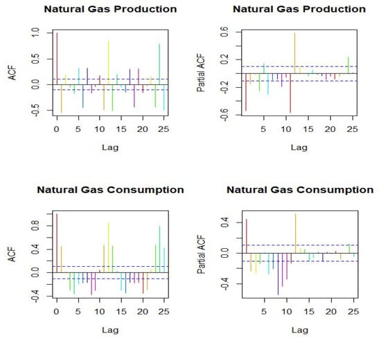
Figure 3. Results of ACF and PACF diagrams for a selection of parameter AR (p) and MA(q) in natural gas production and consumption.

Table 4. Final parameter estimates for the SARIMA model in natural gas production and consumption.

Natural Gas Production
	Training Set			Testing Set
Types of Model Parameter	Coefficient	SE	p-Values	Coefficient	SE	p-Values
AR 1	0.4285	0.124	0.001 ***	-
AR 2	0.0324	0.070	0.645	-
AR 3	0.0368	0.065	0.574	-
AR 4	−0.1234	0.063	0.051 *	-
MA 1	−0.7296	0.130	0.000 ***	-
Seasonal_AR 12	0.9877	0.004	0.000 ***	0.1956	0.215	0.362
Seasonal_MA 12	−0.6532	0.042	0.000 ***	−0.8358	0.272	0.002 ***
Variance (σ2)	1188.9158	-	0.000 ***	1542.1716	-	0.000 ***
Natural Gas Consumption
AR 1	0.5507	0.045	0.000 ***	−0.4870	0.085	0.000 ***
AR 2	0.0391	0.026	0.137	−0.4283	0.086	0.000 ***
MA 1	−0.9944	0.009	0.000 ***	-
Seasonal_AR 12	0.3323	0.051	0.000 ***	−0.6238	0.113	0.000 ***
Seasonal_AR 24	0.1436	0.056	0.010 **	−0.6585	0.108	0.000 ***
Seasonal_AR 36	0.2527	0.047	0.000 ***	−0.5037	0.099	0.000 ***
Seasonal_AR 48	0.1415	0.045	0.002 ***	-
Seasonal_AR 60	0.1172	0.049	0.01 **	-
Variance (σ2)	7394.2535	-	0.00 ***	11030	-	0.000 ***
	Production	Consumption		Production	Consumption
p-values of LB(Q)-test	0.90	0.91		0.96	0.95
p-values of JB-test	0.00	0.00		0.00	0.00
AIC	3570.250	4254.634		901.540	1085.939
BIC	3601.250	4289.509		908.938	1100.734

Authors compilation; Significance level codes; p < 0.001 ***, p < 0.01 **, p < 0.05 * indicate that the null hypothesis is rejected at 1%, 5%, and 10% levels, respectively. SE = standard error; AIC = Akaike information criterion; BIC = Bayesian information criterion.

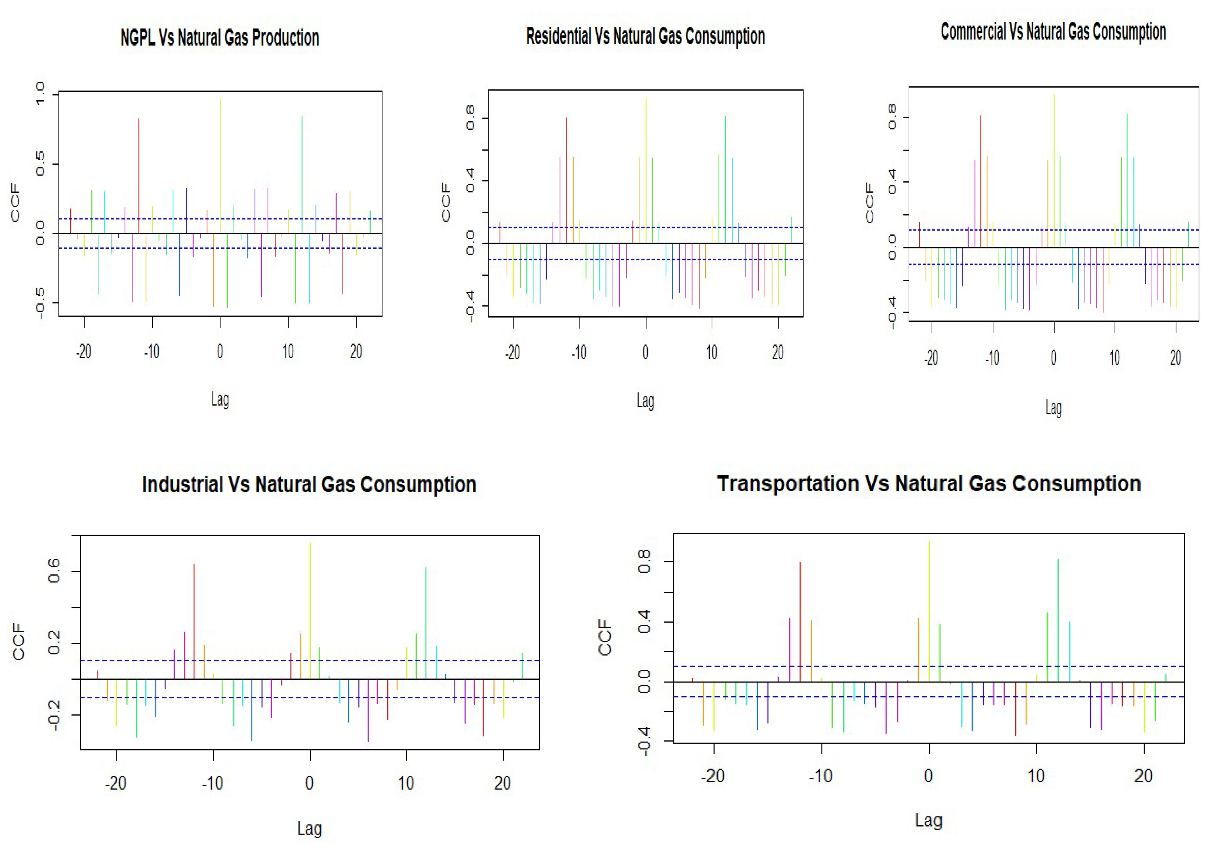
The cross-correlation function (CCF) is used to examine relationships between natural gas production and consumption with other exogenous factors NPGL production, residential, commercial, industrial, and transportation sectors. The CCF between the exogenous variables are monthly NPGL production, residential, commercial, industrial, and transportation is presented in Figure 4. Accepting only positive lags, all of the exogenous variables (NPGL production, residential, commercial, industrial, and transportation) are significantly associated with natural gas production and consumption of at least some of the lags. Similarly, Table 5 presents the best fit model based on significant parameters and coefficient statistics. The p-values are always p > 0.05, and this model's criteria estimation appears statistically significant in the appropriate structure of SARIMAX (X-exogenous variable). The best-fitted model is NG production SARIMAX (2,1,0) * (1,0,2)¹² and consumption SARIMAX (1,1,0) * (1,0,1)¹². Accordingly, the selected lowest values of AIC and BIC are presented in Table 5. These results indicate that NPGL production, residential, commercial, industrial, and transportation sectors at integration I(1) affected natural gas production and consumption at integration I(1) after fitted the time series model. Natural gas production and consumption sectors at integration I(1) (coefficient =20.8187, 0.7572, 1.0017, 1.0670, 7.8810, p < 0.05) show a positive relationship with production and consumption, which was the best fitted SARIMAX model. The sufficiency of the SARIMAX (2,1,0) * (1,0,2)¹² and SARIMAX (1,1,0) * (1,0,1)¹² model is verified by the Ljung–Box (Q) test statistics (0.06, 0.04) for which the p-values (production 0.81, consumption 0.83) are presented in Table 5. The Ljung–Box test exceeds the p-value (0.05), but autocorrelation in the SARIMAX model standardized residual rejects the null hypothesis.

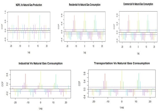
Figure 4. Cross-correlation function with exogenous variables.

Table 5. Final parameter estimates for the SARIMAX (SARIMA with exogenous variables) model in natural gas production and consumption.

Natural Gas Production
	Training Set			Testing Set
Types of Model Parameter	Coefficient	SE	p-Values	Coefficient	SE	p-Values
NGPL Production	20.8187	0.246	0.000 ***	6.5562	0.465	0.000 ***
AR 1	0.8427	0.055	0.000 ***	-
AR 2	0.1232	0.051	0.01 **	-
Seasonal_AR 12	0.6602	0.304	0.030 **	0.9936	0.012	0.000 ***
Seasonal_MA 12	−0.9198	0.301	0.002 ***	−0.7599	0.200	0.000 ***
Seasonal_MA 24	0.2087	0.076	0.006 ***	-
Variance (σ2)	557.2707	-	0.000 ***	941.2649	-	0.000 ***
Natural Gas Consumption
Residential Sector	0.7572	0.162	0.000 ***	0.4840	0.330	0.143
Commercial Sector	1.0017	0.375	0.008 ***	1.5154	0.653	0.020 **
Industrial Sector	1.0670	0.082	0.000 ***	1.3183	0.471	0.005 ***
Transportation Sector	7.8810	0.490	0.000 ***	6.7858	0.802	0.000 ***
AR 1	−0.1212	0.053	0.022 **	-
Seasonal_AR 12	0.9813	0.012	0.000 ***	-
Seasonal_MA 12	−0.6371	0.052	0.000 ***	−0.5583	0.122	0.000 ***
Variance (σ2)	1263.9703	-	0.000 ***	1375.1277	-	0.000 ***
	Production	Consumption		Production	Consumption
p-values of LB(Q)-test	0.81	0.83		0.88	0.39
p-values of JB-test	0.00	0.00		0.00	0.81
AIC	3287.622	3591.060		995.453	892.047
BIC	3314.766	3622.059		1005.834	906.842

Authours compilation; Significance level codes; p < 0.001 ***, p < 0.01 ** indicate that the null hypothesis is rejected at 1%, and 5% levels, respectively. SE = standard error; AIC = Akaike information criterion; BIC = Bayesian information criterion.

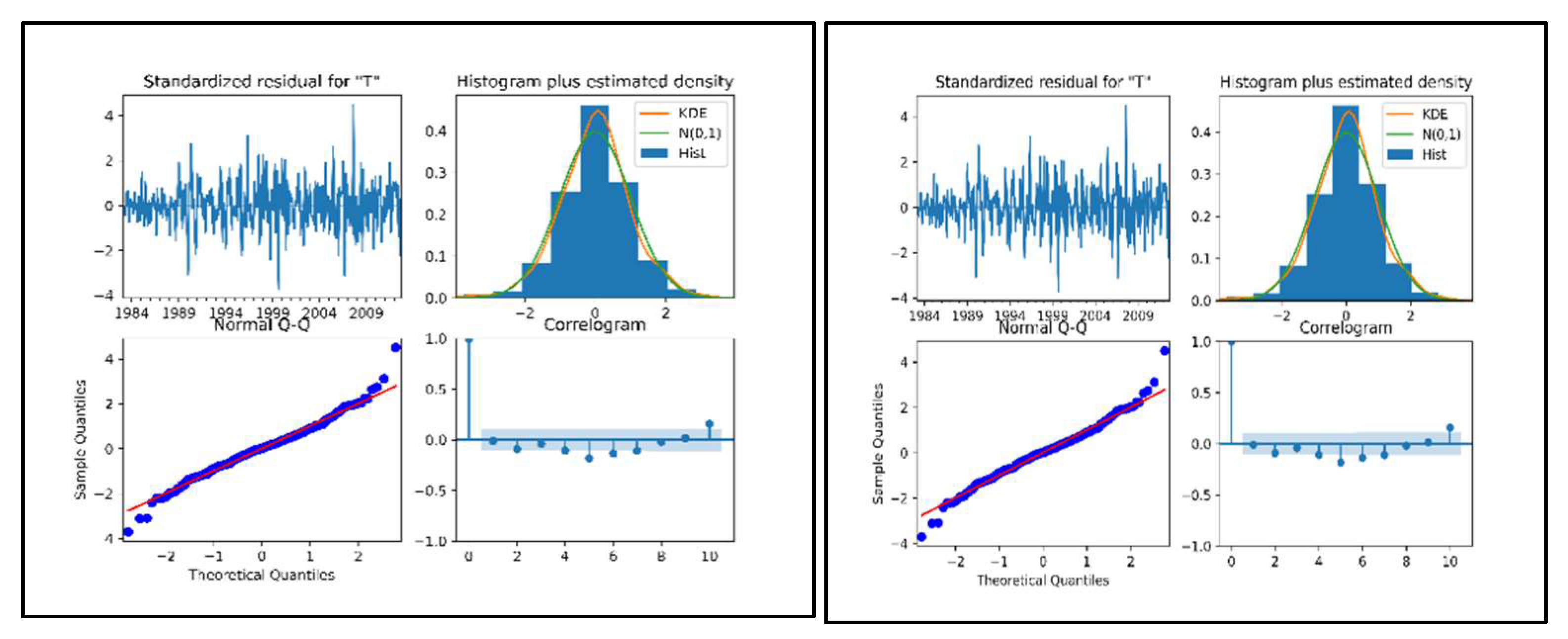
The results show that diagnostic tests on the SARIMAX (2,1,0) * (1,0,2)¹², SARIMAX (1,1,0) * (1,0,1)¹² (right side), SARIMA (4,1,1) * (1,0,1)¹², and SARIMA (2,1,1) * (5,0,0)¹² (left side) are presented in Figure 5 and Figure 6. The correlogram and standardized residual tests (Cryer and Chan 2008) prove that the residual is stationary time series. The Kernel density estimation (KDE) line of the Q-Q plots and histogram plots indicate that the line of the residual follows a normal distribution (Stoffer and Dhumway 2010). These results indicate that the diagnostic statistics test satisfies the inference of SARIMAX and SARIMA modeling of natural gas production and consumption.

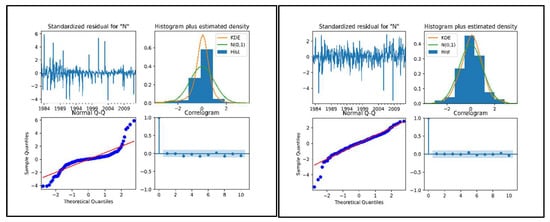
Figure 5. Diagnostic checking of the standardized residuals, histogram, normal Q-Q, and correlogram plots of the SARIMAX (right side) and SARIMA (left side) model for natural gas production.

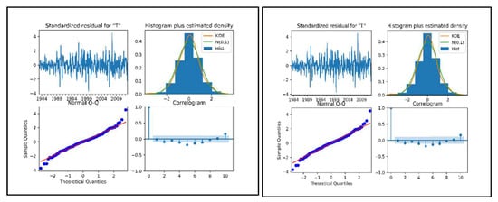
Figure 6. Diagnostic checking of the standardized residuals, histogram, normal Q-Q, and correlogram plots of the SARIMAX (right side) and SARIMA (left side) model for natural gas consumption.

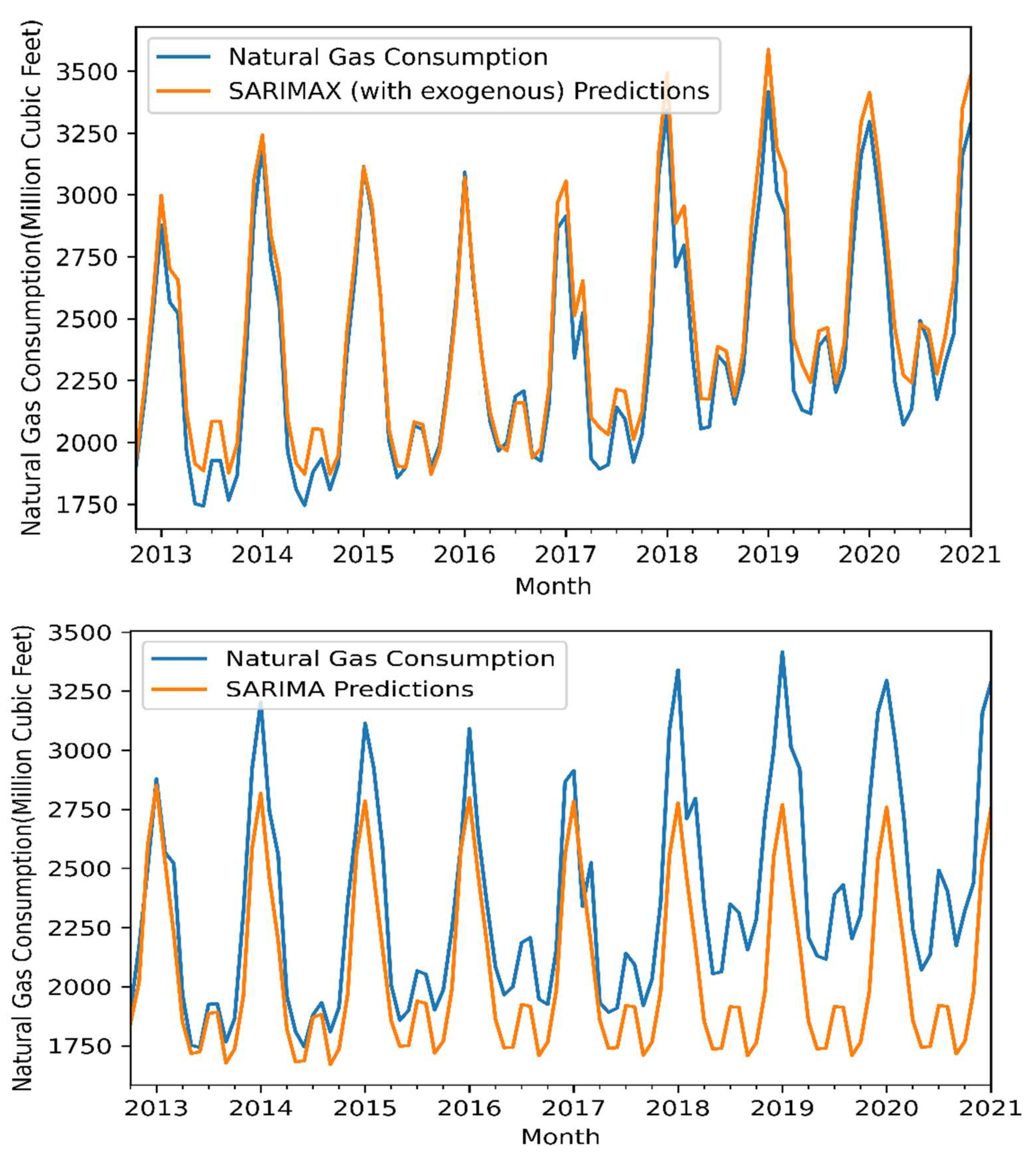
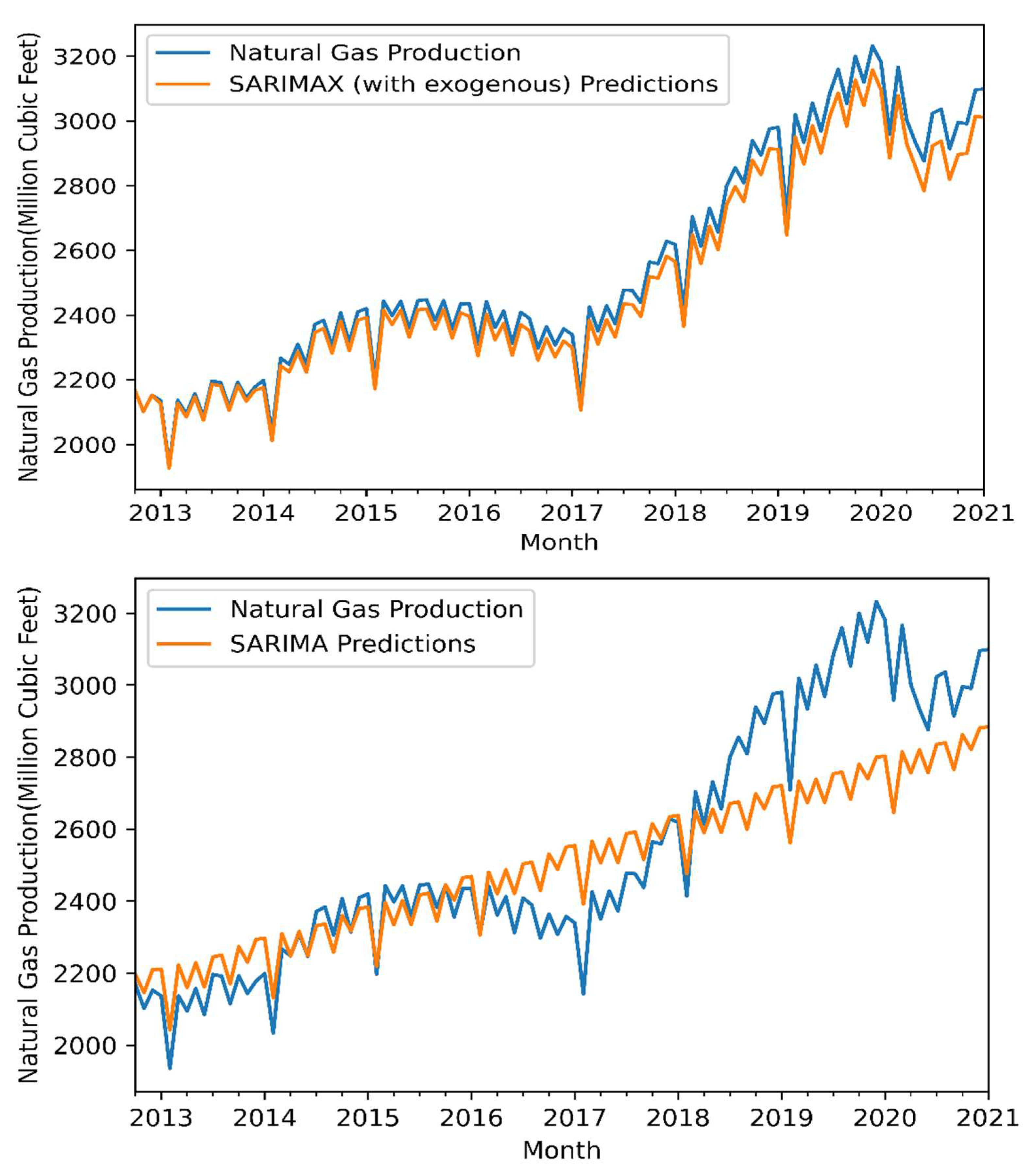
The results were obtained for both sets after using SARIMA and SARIMAX. The received results are presented in Table 6. Furthermore, Figure 7 indicates the production and consumption forecasting performance of these models as a diaram for the test set. Furthermore, although SARIMA models show the best performance than SARIMAX in the training set data, this SARIMAX model shows better performance for the test data set in natural gas production and consumption. In addition, the best performance of SARIMAX is nearby the SARIMA model for the training set. Natural gas production and consumption on the SARIMAX model performance is ‘best’ and ‘well’ according to RMSE and MAPE measures for the training data set, respectively. The SARIMA models have good performance according to RMSE and MAPE measures for the test data set.

Table 6. The performances metrics of the models SARIMA and SARIMAX.

Measure	Training Set (Production)		Test Set (Production)		Training Set (Consumption)		Test Set (Consumption)
	SARIMA	SARIMAX	SARIMA	SARIMAX	SARIMA	SARIMAX	SARIMA	SARIMAX
RMSE	168.46	664.40	3106.47	184.53	131.73	254.76	1636.48	254.45
MAPE	12.75	30.28	125.66	15.93	19.19	20.71	69.45	24.36

Authours compilation; RMSE = root mean square error; MAPE = mean absolute percentage error.

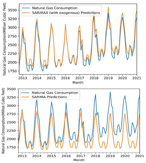
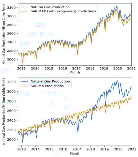
Figure 7. Forecast visualization of natural gas production and consumption with SARIMAX and SARIMA models with selected exogenous factors for the test set.

The SARIMA has not been as successful as the SARIMAX in forecasting the monthly NG production and consumption with the seasonal and trends. SARIMA (p, d, q) * (P, D, Q)^s has six parameters. The various values of previous periods affect the forecast progress. The suggested approach is better evaluation of the SARIMA model. This main aim was identical to reach the SARIMA with exogenous variables.

To examine the forecast performance of the SARIMAX model, another comparison is made with four similar studies from the literature review. These first study authors [64] have achieved a prediction of the best performance with around 8% MAPE measure. In that research, the monthly prediction values for only one year were tested data. Our studies are natural gas forecasting for the long-term in the test data set, and a more robust model was obtained. The second study was [65]. In this study, the researchers achieved a prediction best performance of around 5% MAPE measure. Furthermore, our studies are electricity demand for the long-term data were applied in the modeling set. The third study was [10]. In this study, the researchers achieved a prediction best performance with around 9% MAPE measure. However, our studies are natural gas demand for the long-term data were applied in the tested set. The fourth study was [34]. In this study, the researchers achieved a prediction of best performance with around 0.357% MAPE measure. However, Long-term data were used in the training set. The comparison of the results is presented in Table 7. These results indicated that the SARIMAX is successful on seasonal prediction in a few points.

Table 7. The comparison results for SARIMAX and similarly other papers findings.

Authors	Models	Traning Set	Test Set	MAPE	Prediction For
Akkurt et.al (2010)	SARIMA	1999–2007	2008	7.42	Monthly natural gas
	Winters models			7.83
Hamzacebi (2016)	GM(1,1)	1987–2009	2010–2014	8.39	Monthly electricity demand
	SGM(1,1)			5.18
Es (2021)	ASGM(1,1)	2000–2013	2014–2018	8.67	Monthly natural gas demand
	SGM(1,1)			10.70
	SARIMA			17.99
Yucesan et al. (2021)	NARX	2017–2018	2019	5.346	Daily NG consumption
	ARIMAX-ANN			0.500
	SARIMAX-ANN			0.357
Research paper	SARIMAX (P)	1983–2012	2013–2021	15.93	Monthly NG production and consumption
	SARIMAX (C)	1983–2012	2013–2021	24.36

Authors compilation;. (P) = Production, (C) = Consumption.

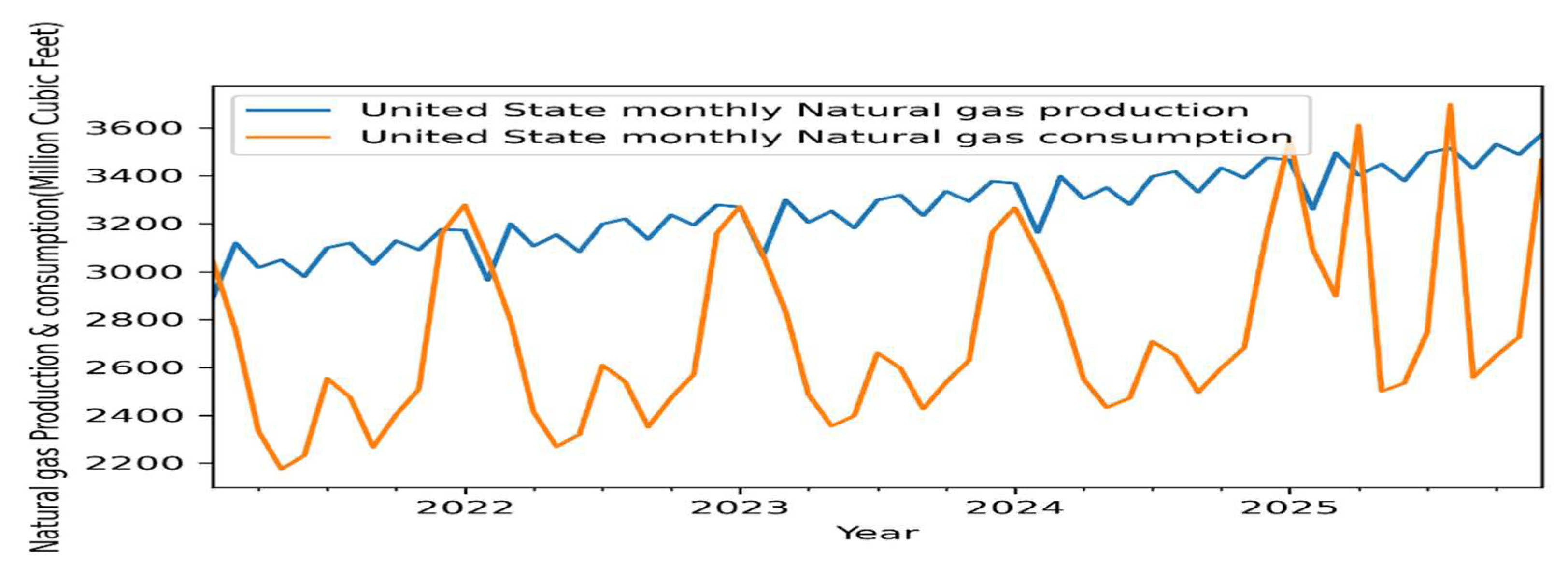
These best-proposed methods have been determined, while the result shows those compared with both models and from similar literature reviews. However, the United States’ monthly natural gas production and consumption until 2025 is forecast by the SARIMAX model as covariates. The prediction values of natural gas production and consumption are presented in Table 8 and indicated in Figure 8. while the results were analyzed, it was evaluated that natural gas production and consumption will be increasing seasonally. The production and consumption increase was a regular condition in light of the industrial, residential, commercial, transportation, population growth, and economic developments in the current years. When the maximal production was conducted in December, the minimum production is in February. Similarly, when the maximal consumption was conducted in January, the minimum is in May. The yearly natural gas production and consumption in 2025 is expected to grow by 16% and 24% compared to 2020 if the seasonal trend continues. In a country that imports all of its natural gas, it is needful to modify the situation and apply different and mostly local energy sources such as nuclear power, coal, and renewable energy.

Table 8. Forecast values on the monthly wise natural gas production and consumption of the United States.

The Monthly Wise Natural Gas Production Prediction of the US Until 2025
Year	Jan.	Feb.	Mar.	Apr.	May	Jun	July	Aug.	Sep.	Oct.	Nov.	Dec.
2021	-	2889	3120	3017	3049	2980	3100	3120	3030	3129	3091	3177
2022	3172	2965	3200	3107	3154	3083	3199	3221	3135	3237	3194	3278
2023	3270	3064	3299	3206	3253	3182	3298	3320	3234	3336	3293	3377
2024	3369	3163	3398	3304	3351	3280	3397	3418	3332	3434	3391	3475
2025	3467	3261	3496	3402	3449	3379	3495	3516	3430	3532	3489	3573
The Monthly Wise Natural Gas Consumption Prediction of the US Until 2025
2021	-	3046	2754	2334	2175	2232	2554	2475	2267	2402	2510	3159
2022	3279	3059	2795	2414	2270	2320	2610	2540	2351	2473	2572	3161
2023	3272	3072	2833	2487	2355	2399	2661	2598	2427	2538	2629	3163
2024	3266	3083	2867	2552	2432	2471	2707	2650	2496	2596	2681	3165
2025	3561	3094	2898	3612	2501	2535	2749	3698	2558	2649	2727	3467

Authors own compilation.

Figure 8. Graph of the United States monthly natural gas production and consumption until 2025.

4. Conclusions and Policy Implications

The future prediction of energy, which is a critical component, is of significance for developed and developing countries. Moreover, it will be feasible to determine future energy policy, plan energy investments, and take necessary precautions. In the short term, there are many benefits to evaluating natural gas production and consumption. In recent years, natural gas evaluations have been made using various methodologies. The most successful forecasting in monthly wise predictions studies can be obtained by improving the seasonal prediction methods. In this study, a new approach which is called the SARIMAX prediction method is recommended for forecasting the United States' monthly wise natural gas production and consumption.

The proposed methods focus on finding the most relevant past observation values by making identical estimations. Moreover, it performs tests for all applicable values on the seasonal coefficient. In this way, seasonality performance in the dataset is more successfully modeled. The success of the model has been detected using some comparisons. Firstly, this method is compared with SARIMA (p, d, q) * (P, D, Q)^s and SARIMAX (p, d, q) * (P, D, Q)^s along with the same dataset. The forecast accuracy measures as RMSE and MAPE results indicate the proposed models were higher than other models. The natural gas production and consumption time series dataset of this study were modeled and improved the forecast performance of the SARIMAX model with RMSE and MAPE values. Moreover, the conquest of the proposed method has been determined by comparing with similar articles related to monthly wise natural gas production and consumption. Finally, by use of the proposed method, monthly wise natural gas production and consumption for the United States was predicted until 2025.

The result shows seasonal fluctuation in the year will be determined with the monthly forecast model, it is feasible to analyze such a situation around seasonal balance, shortage of gas supply, and peak for decision-makers. This study organizes important outputs to the country's energy planning, decision-makers, and energy policies.

Suggestions for future policymakers are given below: (a) Establish a useful natural predict model that will play a key role in determining future gas purchase agreements, liquefied natural gas (LNG) and natural gas storage applications, consumption, production, and storage planning of renewable energy and other fossil energy sources, and finally, the country’s energy policies; (b) improving on-demand flexibility and performance; (c) sustaining and enhancing infrastructure; (d) supporting energy sectors innovation; (e) accelerating the uses of sustainable energy, utilization, and carbon capture technologies; (f) invest in a long-term perspective and safe areas in nuclear energy; (g) policymakers need methods to measure and evaluate the current and future effects of energy use on human society, human health, water, soil, and air; (h) achieving sustainable development requires appropriate energy policy formulation, political, economic, social, and environmental considerations; (i) energy geography is evolving significantly, which requires a focus on analyzing patterns of energy supply and demand.

References

- Lu, H.; Ma, X.; Azimi, M. US natural gas consumption prediction using an improved kernel-based nonlinear extension of the Arps decline model. Energy 2020, 194, 116905. [Google Scholar] [CrossRef]
- Deng, Q.; Alvarado, R.; Toledo, E.; Caraguay, L. Greenhouse gas emissions, non-renewable energy consumption, and output in South America: The role of the productive structure. Environ. Sci. Pollut. Res. 2020, 27, 14477–14491. [Google Scholar] [CrossRef]
- Sen, D.; Günay, M.E.; Tunç, K.M.M. Forecasting annual natural gas consumption using socio-economic indicators for making future policies. Energy 2019, 173, 1106–1118. [Google Scholar] [CrossRef]
- BP. Energy Outlook, 2020th ed.; Linda Capuano: EIA, Today in Energy; 20 April 2020. Available online: https://www.eia.gov/todayinenergy/detail.php?id=43395 (accessed on 15 July 2021).
- Deetman, S.; Hof, A.F.; Pfluger, B.; van Vuuren, D.P.; Girod, B.; van Ruijven, B.J. Deep greenhouse gas emission reductions in Europe: Exploring different options. Energy Policy 2013, 55, 152–164. [Google Scholar] [CrossRef] [Green Version]
- Murshed, M.; Alam, R.; Ansarin, A. The environmental Kuznets curve hypothesis for Bangladesh: The importance of natural gas, liquefied petroleum gas, and hydropower consumption. Environ. Sci. Pollut. Res. 2021, 28, 17208–17227. [Google Scholar] [CrossRef] [PubMed]
- Riazi, M.R. Energy, economy, environment and sustainable development in the Middle East and North Africa. Int. J. Oil Gas Coal Technol. 2010, 3, 201–244. [Google Scholar] [CrossRef]
- Ravnik, J.; Hriberšek, M. A method for natural gas forecasting and preliminary allocation based on unique standard natural gas consumption profiles. Energy 2019, 180, 149–162. [Google Scholar] [CrossRef]
- Lakatos, I.; Julianna, L.S. Global oil demand and role of chemical EOR methods in the 21st century. Int. J. Oil Gas Coal Technol. 2008, 1, 46–64. [Google Scholar] [CrossRef]
- Es, H.A. Monthly natural gas demand forecasting by adjusted seasonal grey forecasting model. Energy Sources Part A Recover. Util. Environ. Eff. 2021, 43, 54–69. [Google Scholar] [CrossRef]
- Karakurt, I. Modelling and forecasting the oil consumptions of the BRICS-T countries. Energy 2021, 220, 119720. [Google Scholar] [CrossRef]
- Al-Fattah, S.M.; Aramco, S. Application of the artificial intelligence GANNATS model in forecasting crude oil demand for Saudi Arabia and China. J. Pet. Sci. Eng. 2021, 200, 108368. [Google Scholar] [CrossRef]
- British Petroleum (BP). BP Statistical Review of World Energy, 69th ed.; British Petroleum Co.: London, UK, 2020. [Google Scholar]
- Suganthi, L.; Samuel, A.A. Energy models for demand forecasting—A review. Renew. Sustain. Energy Rev. 2012, 16, 1223–1240. [Google Scholar] [CrossRef]
- Pi, D.; Liu, J.; Qin, X. A grey prediction approach to forecasting energy demand in China. Energy Sources Part A Recover. Util. Environ. Eff. 2010, 32, 1517–1528. [Google Scholar] [CrossRef]
- Liu, J.; Wang, S.; Wei, N.; Chen, X.; Xie, H.; Wang, J. Natural gas consumption forecasting: A discussion on forecasting history and future challenges. J. Nat. Gas Sci. Eng. 2021, 90, 103930. [Google Scholar] [CrossRef]
- Anđelković, A.S.; Bajatović, D. Integration of weather forecast and artificial intelligence for a short-term city-scale natural gas consumption prediction. J. Clean. Prod. 2020, 266, 122096. [Google Scholar] [CrossRef]
- Chen, Y.; Xu, X.; Koch, T. Day-ahead high-resolution forecasting of natural gas demand and supply in Germany with a hybrid model. Appl. Energy 2020, 262, 114486. [Google Scholar] [CrossRef]
- Karadede, Y.; Ozdemir, G.; Aydemir, E. Breeder hybrid algorithm approach for natural gas demand forecasting model. Energy 2017, 141, 1269–1284. [Google Scholar] [CrossRef]
- Sánchez-Úbeda, E.F.; Berzosa, A. Modeling and forecasting industrial end-use natural gas consumption. Energy Econ. 2007, 29, 710–742. [Google Scholar] [CrossRef]
- Karabiber, O.A.; Xydis, G. Forecasting day-ahead natural gas demand in Denmark. J. Nat. Gas Sci. Eng. 2020, 76, 103193. [Google Scholar] [CrossRef]
- Khotanzad, A.; Elragal, H. Natural gas load forecasting with combination of adaptive neural networks. Proc. Int. Jt. Conf. Neural Netw. 1999, 6, 4069–4072. [Google Scholar] [CrossRef]
- Khotanzad, A.; Elragal, H.; Lu, T.L. Combination of artificial neural-network forecasters for prediction of natural gas consumption. IEEE Trans. Neural Netw. 2000, 11, 464–473. [Google Scholar] [CrossRef] [PubMed]
- Hippert, H.S.; Pedreira, C.E.; Souza, R.C. Neural networks for short-term load forecasting: A review and evaluation. IEEE Trans. Power Syst. 2001, 16, 44–55. [Google Scholar] [CrossRef]
- Lu, H.; Cheng, F.; Ma, X.; Hu, G. Short-term prediction of building energy consumption employing an improved extreme gradient boosting model: A case study of an intake tower. Energy 2020, 203, 117756. [Google Scholar] [CrossRef]
- Soldo, B. Forecasting natural gas consumption. Appl. Energy 2012, 92, 26–37. [Google Scholar] [CrossRef]
- Lu, H.; Azimi, M.; Iseley, T. Short-term load forecasting of urban gas using a hybrid model based on improved fruit fly optimization algorithm and support vector machine. Energy Rep. 2019, 5, 666–677. [Google Scholar] [CrossRef]
- Kinateder, H.; Campbell, R.; Choudhury, T. Safe haven in GFC versus COVID-19: 100 turbulent days in the financial markets. Financ. Res. Lett. 2021, 101951, in press. [Google Scholar] [CrossRef]
- Qiao, W.; Yang, Z.; Kang, Z.; Pan, Z. Short-term natural gas consumption prediction based on Volterra adaptive filter and improved whale optimization algorithm. Eng. Appl. Artif. Intell. 2020, 87, 103323. [Google Scholar] [CrossRef]
- Soldo, B.; Potočnik, P.; Šimunović, G.; Šarić, T.; Govekar, E. Improving the residential natural gas consumption forecasting models by using solar radiation. Energy Build. 2014, 69, 498–506. [Google Scholar] [CrossRef]
- Brabec, M.; Konár, O.; Pelikán, E.; Malý, M. A nonlinear mixed effects model for the prediction of natural gas consumption by individual customers. Int. J. Forecast. 2008, 24, 659–678. [Google Scholar] [CrossRef]
- Taşpinar, F.; Çelebi, N.; Tutkun, N. Forecasting of daily natural gas consumption on regional basis in Turkey using various computational methods. Energy Build. 2013, 56, 23–31. [Google Scholar] [CrossRef]
- Hošovský, A.; Piteľ, J.; Adámek, M.; Mižáková, J.; Židek, K. Comparative study of week-ahead forecasting of daily gas consumption in buildings using regression ARMA/SARMA and genetic-algorithm-optimized regression wavelet neural network models. J. Build. Eng. 2021, 34, 101955. [Google Scholar] [CrossRef]
- Yucesan, M.; Pekel, E.; Celik, E.; Gul, M.; Serin, F. Forecasting daily natural gas consumption with regression, time series and machine learning based methods. Energy Sources Part A Recover. Util. Environ. Eff. 2021, 00, 1–16. [Google Scholar] [CrossRef]
- Zhou, H.; Su, G.; Li, G. Forecasting daily gas load with OIHF-Elman neural network. Procedia Comput. Sci. 2011, 5, 754–758. [Google Scholar] [CrossRef] [Green Version]
- Demirel, Ö.F.; Zaim, S.; Çališkan, A.; Özuyar, P. Forecasting natural gas consumption in Istanbul using neural networks and multivariate time series methods. Turkish J. Electr. Eng. Comput. Sci. 2012, 20, 695–711. [Google Scholar] [CrossRef]
- Wang, R.; Lu, S.; Feng, W. A novel improved model for building energy consumption prediction based on model integration. Appl. Energy 2020, 262, 114561. [Google Scholar] [CrossRef]
- Zhang, P.G. Time series forecasting using a hybrid ARIMA and neural network model. Neurocomputing 2003, 50, 159–175. [Google Scholar] [CrossRef]
- Ediger, V.Ş.; Akar, S. ARIMA forecasting of primary energy demand by fuel in Turkey. Energy Policy 2007, 35, 1701–1708. [Google Scholar] [CrossRef]
- Bierens, H.J. Armax model specification testing, with an application to unemployment in the Netherlands. J. Econom. 1987, 35, 161–190. [Google Scholar] [CrossRef]
- Jalalkamali, A.; Moradi, M.; Moradi, N. Application of several artificial intelligence models and ARIMAX model for forecasting drought using the Standardized Precipitation Index. Int. J. Environ. Sci. Technol. 2015, 12, 1201–1210. [Google Scholar] [CrossRef] [Green Version]
- Box, G.E.; Jenkins, G.M.; MacGregor, J.F. Some recent advances in forecasting and control. J. R. Stat. Soc. Ser. C (Appl. Stat.) 1974, 23, 158–179. [Google Scholar] [CrossRef]
- Cools, M.; Moons, E.; Wets, G. Investigating the variability in daily traffic counts through use of ARIMAX and SARIMAX models: Assessing the effect of holidays on two site locations. Transp. Res. Rec. 2009, 2136, 57–66. [Google Scholar] [CrossRef] [Green Version]
- Hipel, K.W.; McLeod, A.I. Chapter 12 seasonal autoregressive integrated moving average models. Dev. Water Sci. 1994, 45, 419–462. [Google Scholar] [CrossRef]
- Box, G.E.; Jenkins, G.M. Some recent advances in forecasting and control. J. R. Stat. Soc. Ser. C (Appl. Stat.) 1968, 17, 91–109. [Google Scholar] [CrossRef]
- Bartholomew, D.J. Review of Time Series Analysis Forecasting and Control., by G. E. P. Box & G. M. Jenkins. Oper. Res. Q. (1970–1977) 1971, 22, 199–201. [Google Scholar] [CrossRef]
- Nau, R. Mathematical structure of ARIMA models. Duke Univ. Online Artic. 2014, 1, 1–8. [Google Scholar]
- Box, G.E.; Jenkins, G.M.; Reinsel, G.C.; Ljung, G.M. Time Series Analysis: Forecasting and Control; John Wiley & Sons: Hoboken, NJ, USA, 2015. [Google Scholar]
- Hamzaçebi, C. Improving artificial neural networks’ performance in seasonal time series forecasting. Inf. Sci. 2008, 178, 4550–4559. [Google Scholar] [CrossRef]
- Tarsitano, A.; Amerise, I.L. Short-term load forecasting using a two-stage sarimax model. Energy 2017, 133, 108–114. [Google Scholar] [CrossRef]
- Dutta, J.; Roy, S. IndoorSense: Context based indoor pollutant prediction using SARIMAX model. Multimed. Tools Appl. 2021, 80, 19989–20018. [Google Scholar] [CrossRef]
- Hao, Y.; Wang, R.R.; Han, L.; Wang, H.; Zhang, X.; Tang, Q.L.; Yan, L.; He, J. Time series analysis of mumps and meteorological factors in Beijing, China. BMC Infect. Dis. 2019, 19, 1–10. [Google Scholar] [CrossRef]
- Duan, Y.; Huang, X.L.; Wang, Y.J.; Zhang, J.Q.; Zhang, Q.; Dang, Y.W.; Wang, J. Impact of meteorological changes on the incidence of scarlet fever in Hefei City, China. Int. J. Biometeorol. 2016, 60, 1543–1550. [Google Scholar] [CrossRef]
- Pepple, S.U.; Harrison, E.E. Comparative performance of Garch and Sarima techniques in the modeling of Nigerian board money. CARD Int. J. Soc. Sci. Confl. Manag. 2017, 2, 258–270. [Google Scholar]
- Armstrong, J.S.; Collopy, F. Error measures for generalizing about forecasting methods: Empirical comparisons. Int. J. Forecast. 1992, 8, 69–80. [Google Scholar] [CrossRef] [Green Version]
- Hyndman, R.J.; Koehler, A.B. Another look at measures of forecast accuracy. Int. J. Forecast. 2006, 22, 679–688. [Google Scholar] [CrossRef] [Green Version]
- Zhang, X.; Pang, Y.; Cui, M.; Stallones, L.; Xiang, H. Forecasting mortality of road traffic injuries in China using seasonal autoregressive integrated moving average model. Ann. Epidemiol. 2015, 25, 101–106. [Google Scholar] [CrossRef]
- Elliott, G.; Rothenberg, T.; Stock, J. Efficient Tests for an Autoregressive Unit Root. Econometrica 1996, 64, 813–836. [Google Scholar] [CrossRef] [Green Version]
- Dickey, D.; Fuller, W. Likelihood Ratio Statistics for Autoregressive Time Series with a Unit Root. Econom. J. Econom. Soc. 1981, 49, 1057–1072. [Google Scholar] [CrossRef]
- Dickey, D.A.; Fuller, W.A. Distribution of the Estimators for Autoregressive Time Series With a Unit Root. J. Am. Stat. Assoc. 1979, 74, 427. [Google Scholar] [CrossRef]
- Kwiatkowski, D.; Phillips, P.C.B.; Schmidt, P.; Shin, Y. Testing the null hypothesis of stationarity against the alternative of a unit root. How sure are we that economic time series have a unit root? J. Econom. 1992, 54, 159–178. [Google Scholar] [CrossRef]
- Perron, P. Testing for a unit root in a time series with a changing mean. J. Bus. Econ. Stat. 1990, 8, 153–162. [Google Scholar] [CrossRef]
- Phillips, P.C.; Perron, P. Testing for a Unit Root in Time Series Regression. Biometrika 1988, 75, 335–346. [Google Scholar] [CrossRef]
- Ozden, K.; Yilmaz, I. An Attempt at Pseudo-Democracy and Tactical Liberalization in Turkey: An Analysis of Ismet Inönü’s Decision to Transition to a Multi-Party Political System. Eur. J. Econ. Political Stud. 2010, 3, 189–205. [Google Scholar] [CrossRef]
- Hamzaçebi, C. Primary energy sources planning based on demand forecasting: The case of Turkey. J. Energy S. Afr. 2016, 27, 2–10. [Google Scholar] [CrossRef] [Green Version]
Publisher’s Note: MDPI stays neutral with regard to jurisdictional claims in published maps and institutional affiliations. |
© 2021 by the authors. Licensee MDPI, Basel, Switzerland. This article is an open access article distributed under the terms and conditions of the Creative Commons Attribution (CC BY) license (https://creativecommons.org/licenses/by/4.0/).