Abstract
The current practice for multi-fractured horizontal well development in low-permeability reservoirs is to complete the full length of the well with evenly spaced fracture stages. Given methods to evaluate along-well variability in reservoir quality and to predict stage-by-stage performance, it may be possible to reduce the number of stages completed in a well without a significant sacrifice in well performance. Provision and demonstration of these methods is the goal of the current two-part study. In Part 1 of this study, reservoir and completion quality were evaluated along the length of a horizontal well in the Montney Formation in western Canada. In the current (Part 2) study, the along-well reservoir property estimates are first used to forecast per-stage production variability, and then used to evaluate production performance of the well when fewer stages are completed in higher quality reservoir. A rigorous and fast semi-analytical model was used for forecasting, with constraints on fracture geometry obtained from numerical model history matching of the studied Montney well flowback data. It is concluded that a significant reduction in the number of stages from 50 (what was implemented) to less than 40 could have yielded most of the oil production obtained over the forecast period.
1. Introduction
Multi-fractured horizontal wells (MFHWs) are the most common technology used for economic development of low- and ultra-low (“unconventional”) permeability oil and gas reservoirs. This technology has enabled production from reservoirs that have been traditionally viewed as “non-pay”, with permeabilities in the 10 s to 100 s of nanodarcy range. In modern development practices, MFHWs are commonly drilled from the same pad, often targeting more than one (vertical) reservoir interval in an unconventional play. Another common practice is to place fracturing stages uniformly (or geometrically) along a well; multiple perforation clusters, used as initiation points for hydraulic fractures, are also often used, with the cluster spacing typically constant within a fracture stage. While this practice has generally resulted in commercially successful development of unconventional resources, it can also be inefficient because often only a fraction of the perforation clusters may contribute to hydrocarbon flow, due in part to heterogeneity in reservoir properties along the lateral [1,2].
As a result of the “geometric” fracturing approach (no selective stimulation), and historical lack of focus on along-well reservoir characterization, production forecasting approaches have also typically assumed reservoir/hydraulic fracture homogeneity along a well. It is common practice to use “element of symmetry” (single fracture or quarter fracture) models, that are then scaled up to the total number of fractures (estimated based on perforation cluster efficiency) to generate a production forecast of a MFHW. A number of approaches have been used to generate forecasts for MFHWs, which can be classified as empirical [3,4,5,6], analytical [7,8,9,10,11], semi-analytical [12], or hybrid [13,14] methods. Clarkson et al. [15] applied a combination of these approaches for forecasting MFHWs.
The goal of this two-part study is therefore to demonstrate a workflow for improving well stimulation effectiveness through the selection of higher reservoir quality intervals along the well for stimulation, and comparison of the forecasts for these selected intervals with the forecast for the well using a geometric fracturing approach. The workflow consists of the following steps: (1) quantify reservoir quality (RQ) and completion quality (CQ) along a horizontal well, as determined from a combination of petrophysical, geochemical and geomechanical properties; (2) identify intervals of higher RQ/CQ that can be selected for stimulation; (3) use a simulation model, populated with properties determined from step 1, to generate production forecasts for all stages of the well (assuming a geometric fracturing approach); (4) compare the production forecast for the selected (higher RQ/CQ) intervals against the production forecast for all intervals (geometric fracturing case) to determine if fewer stages can be completed in the well without significant loss in well performance. Previous approaches for Steps 1 and 2 have been discussed in the literature e.g., [16,17,18,19,20,21]. If Step 4 results in the conclusion that fewer fracturing stages can be implemented, and if the reduction of cost for stimulation outweighs the consequent loss in production, then more efficient development, with lower environmental impact (less water and sand use, lower surface footprint), can be achieved. Steps 1 and 2 of the workflow are the subject of the Part 1 paper [22], while steps 3 and 4 are the subject of the current (Part 2) paper.
In the Part 1 study, petrophysical and geomechanical properties generated from well logs, petrophysical, geochemical and rock type information (using petrographic analysis) derived from drill cuttings analysis, and geomechanical information derived from drilling data, were integrated to enable the quantification of RQ/CQ along a horizontal well drilled in the Montney Formation of western Canada (Step 1 of the workflow). Cutoff criteria were defined and applied to identify RQ/CQ “sweetspots” (Step 2 of the workflow).
In order to implement Steps 3 and 4 of the workflow (applied to the same MFHW as the Part 1 study), a semi-analytical model, which uses the dynamic drainage area (DDA) concept and was developed for history-matching flowback and early time production of MFHWs [23], is selected. This model is used for individual stage forecasting, as opposed to fully numerical simulation, because it is quick and easy to setup and has faster run times than numerical simulation, which is desirable when many intervals require a forecast in a short period of time. However, prior to the use of the DDA model for stage-level forecasting, a fully numerical compositional simulator, with properties imported from a 3D geological model constructed for a region around the well, was used to history match the subject well production rates, flowing bottomhole pressures, and gas composition data during the flowback period in order to derive estimates of the fracture properties to be used in the DDA model. While the DDA model does include a hydraulic fracture modeling module that can be used to estimate fracture properties from the stimulation treatment data for each stage (see Zhang et al. [23] for model details), given various petrophysical and geomechanical property input, the fracture model is currently slow to run. Therefore, for this proof-of-concept study, hydraulic fracture properties are fixed for each stage (using the results of the numerical model history match); any production forecast variability is therefore attributed to reservoir properties selected for that stage.
For this Part 2 (proof-of-concept) study, reservoir modeling is implemented in the following steps: (1) history match subject well flowback data using a compositional numerical model in order to estimate hydraulic fracture properties (e.g., height and length); (2) use the semi-analytical DDA model, constrained by fracture properties derived from the numerical model history match, to forecast stage production for 15 stages with variable RQ/CQ (as determined from the Part 1 study) in order to assess the range in production performance associated with these stages; (3) forecast production for all of the (50) stages of the well; (4) compare production forecasts for a subset of higher RQ/CQ stages to the production from all stages (geometric fracturing case). The results of these steps, as applied to the same Montney Formation MFHW studied in Part 1 [22], will be discussed and the efficacy of selective stimulation evaluated.
2. Theory and Methods
In this section, the geologic model and numerical model setup and procedure used to history-match flowback data of the subject MFHW are first described. This calibrated numerical model is used to estimate the fracture height and half length, which in turn is used for individual stage forecasting with the semi-analytical (DDA) model. Next, a brief description of the semi-analytical model used for individual stage forecasting, and for the comparison between the geometric fracturing (all stages) and selected stages production forecast, is provided.
2.1. Numerical Model History Match of Flowback Rates and Gas Compositions
A fully numerical simulation model was generated to estimate the fracture geometry (height and length) created by the hydraulic fracture stimulation by history matching the flowback rates, flowing bottomhole pressures, and surface gas composition data of the subject MFHW. To minimize simulation runtimes, identical fracture dimensions, and reservoir volume attached to each fracture, were assumed, and only a single stage (element of symmetry) was modeled. In the following, the geologic model used to derive petrophysical data input for the simulation model is first described, followed by the numerical model setup and history-matching procedure.
2.1.1. Geological Model
A 3D stochastic model was created using the PetrelTM software. A detailed description of the model construction workflow was provided in Clarkson et al. [24]. For the sake of completeness, a brief summary is provided herein. The created geomodel area includes the studied MFHW and neighboring MFHW and vertical wells. The model was finely gridded (75 m × 75 m × 1.6 m; 2.1 million active grid cells), and grid orientation (−0.45°) was aligned with the interpreted paleo-shelf edge orientation and regional depositional trends. Because of the relatively fine vertical gridding (137 geological layers), vertical heterogeneity in the reservoir is reasonably captured. The horizons were created using the “Make Horizon” process in PetrelTM and gamma-ray (GR) cutoffs were used for facies modeling and distribution. As part of the petrophysical modeling process, 3D models of porosity and permeability in the reservoir were generated. Log-derived porosities used in the petrophysical modeling were first adjusted to match core data [25] and then were scaled up to the 3D grid using an arithmetic average method in PetrelTM. Next, a 3D porosity distribution was generated using the sequential Gaussian simulation technique in PetrelTM. For permeability modeling, profile permeability, scaled-up to log scale using the procedure of Clarkson et al. [26], and corrected to in situ stress, was cross-plotted against log-calculated porosity. This relationship was used to generate a 3D grid for reservoir permeability.
2.1.2. Reservoir Simulation Model Setup
A 3D numerical simulation model was constructed in the CMG® GEMTM compositional reservoir simulator and used to estimate fracture geometry by history matching flowback production rates, flowing bottomhole pressures, and surface gas composition data.
A small 3D sub-section of the original geologic model (sector model) was imported into the simulation model for use in history matching flowback data. A small model is appropriate for the matching of flowback data because the flowback production period lasts for only 20 days, resulting in only a small distance of investigation in the reservoir. Only one stage is modeled (element of symmetry). Porosity upscaling in the vertical direction reduced the number of vertical layers from 137 to 26. An average porosity value was assumed for each layer in the model, removing the effects of lateral heterogeneity, i.e., a cube model (vertically heterogeneous, laterally homogeneous) was used for simulation. The aforementioned porosity-permeability relationship was used to generate the permeability distribution in the reservoir model. Water saturation was assumed to be constant and uniform for each layer. In order to capture the full fracture height growth, the reservoir model was extended to include the entire Montney Formation, as well as a fraction of the overlying Doig and underlying Belloy formations.
A logarithmic refinement was used inside the grid blocks that host the hydraulic fracture (HF) to accurately model the pressure and saturation changes in grids near the HF. A stimulated reservoir volume (SRV) with elevated permeability adjacent to the HF is also considered in this work following Hamdi et al. [27]. This is a common engineering practice for modeling tight oil/gas reservoirs [10,11,12,27,28] to account for fracture complexity.
The in situ fluid composition within the model was estimated by recombining the separator oil compositions with the gas compositions determined by sampling the headspace of isojars® containing cuttings samples captured from the Doig, Montney, and Belloy formations. The cuttings samples were collected from an offset vertical well in 10 m intervals. Therefore, the numerical model accounted for vertical heterogeneity in fluid compositions on initialization. The separator gas–oil ratio (GOR) value required for recombination calculations was not available, and hence was used as a history match parameter in this study. The combination of the vertical heterogeneity in in situ fluid composition used for model initialization, and history matching of surface gas compositions, was used to constrain the height of the hydraulic fracture, as explained by Clarkson et al. [24]. The fluid recombination technique is outlined by McCain [29] and also explained in detail by Clarkson et al. [24].
A planar HF with a constant 3.048 × 10⁻⁴ m width was used in this work and treated as a propped fracture with effective porosity, permeability, length, and height properties. These unknown HF properties, along with the initial water saturation in the HF, were estimated as part of the history-matching procedure described below. Laboratory measured propped fracture permeability values as a function of stress [30] were used to estimate HF permeability changes with pressure in the simulation model. The use of these lab data to constrain the simulation model significantly improved the quality of the history-matching (HM) results. Non-Darcy flow due to inertia in the HF [31] was simulated using the CMG GEM default correlation.
Different relative permeability curves were assumed for the HF and SRV regions in the model. The Brooks and Corey [32] two-phase, and Stone II [33] three-phase, relative permeability models were used to simulate multiphase flow in the model. The parameters of the Brooks-Corey correlations were estimated through the history-matching process. SRV and matrix (unstimulated reservoir) relative permeability curves were assumed to be the same. Capillary pressure was ignored in this study for all three regions.
2.1.3. Simulation History-Matching Procedure
Nineteen parameters in the model were adjusted to achieve a history match of flowback production rates, flowing bottomhole pressures (BHPs), and surface gas compositions, in order to estimate HF, SRV, matrix and fluid properties.
Due to significant changes in the GOR during flowback, 4 different values were used in the history-matching process to initialize the in situ fluid compositions. The height of the fracture is represented by the number of grids above and below the horizontal well. The maximum number of grids above the horizontal well is 9, which covers the entire Upper Montney and part of the Doig Formation. Similarly, the entire Lower Montney, and a portion of the Belloy Formation, is covered with 10 grid blocks below the horizontal well.
The initial water saturation inside the SRV region is calculated by honoring the following material balance equation:
where is the total volume of water injected into the formation during the hydraulic fracture stimulation treatment, is porosity, is water saturation, is fracture half-length, is fracture height, is fracture width, and is the extension of SRV along the horizontal well.
The total fluid production of the subject MFHW is the main constraint applied to the simulation model, while individual fluid rates and BHP data were history matched by minimizing the following global objective function. [34]:
where is the weight factor and is a local error. A higher weight factor was assigned to the oil phase ) compared to other parameters in Equation (2).
The history-matching task was completed using the Differential Evolution module (DE) of CMG CMOSTTM with scaling factor, crossover rate, and population size values of 0.5, 0.8, and 35, respectively. Differential Evolution is a population-based metaheuristic optimization technique [35] which can be applied to high-dimensional oil and gas engineering problems [36,37,38,39,40,41]. A detailed discussion of DE algorithm can be found in Price et al. [42].
2.2. Individual Stage Forecasting Using Semi-Analytical DDA Model
Petrophysical properties (porosity, permeability and water saturation), derived from the along-well reservoir characterization work performed in the Part 1 study [22], and averaged over the length of each fracture stage, were used as input into a semi-analytical model for individual stage forecasting. In the following, the semi-analytical model used for this purpose is first described, and the specific procedure used for forecasting each stage is provided.
Semi-Analytical Model
The semi-analytical model used in this study is based on the dynamic drainage area (DDA) approach, which was first applied to flowback data by Clarkson et al. [12], and subsequently modified by Zhang et al. [23]. The model is capable of simulating two-phase flow (oil and water) for a black oil system. The Zhang et al. [23] version of the model is capable of simulating hydraulic fracture propagation (using a hydraulic fracture simulator), leakoff during the stimulation treatment and subsequent shut-in, as well as flowback. The version used in this work simulates flowback production only from a single fracturing stage.
A conceptual model illustrating the fracture and reservoir regions used in the DDA model is provided in Figure 1. The fracturing stage is subdivided into a primary hydraulic fracture (PHF), and adjacent reservoir region consisting of either an enhanced fracture region (EFR) or a non-stimulated reservoir (NSR) region. The PHF is a single-porosity fracture region assumed to contain most of the proppant and represents the conductive fracture. Three options for the reservoir region can be applied: (1) a single-porosity NSR, representing the native, non-stimulated reservoir with matrix properties; (2) a single-porosity EFR, in which the permeability and porosity are elevated with respect to the matrix; or (3) a dual-porosity EFR, which is composed of two media, a fracture network and matrix blocks, where the unpropped fracture network is assumed to be created as a result of natural fracture reactivation during the hydraulic stimulation treatment.
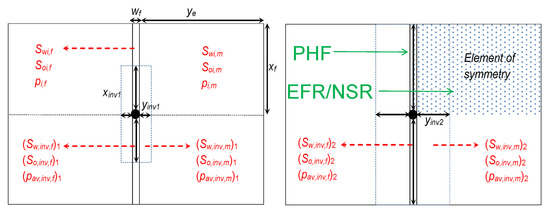
Figure 1.
Conceptual model used by Clarkson et al. [12] for the tight oil DDA model. The conceptual model assumes that each hydraulic fracturing stage has a primary hydraulic fracture, containing most of the proppant, and two reservoir regions, adjacent to the primary hydraulic fracture. Modified from Clarkson et al. [43].
Illustrated in Figure 1 is the dynamic drainage area propagation within the PHF and EFR/NSR at early time (Figure 1, left), and within the EFR/NSR at later time (Figure 1, right). Transient linear flow within each region is modeled using the succession of pseudosteady states concept [44]. The drainage area of each region in the direction of flow during transient linear flow is calculated using the linear flow distance of investigation (DOI) equation. The conceptual model in Figure 1 assumes that pressure in the PHF and EFR/NSR are equal at the start of production. At early time (Figure 1, left), the DDA propagates within the PHF and EFR/NSR simultaneously. At later time, after the pressure transient has reached the tip of the PHF, the DDA propagates within the EFR/NSR only.
While the mathematical model for production during flowback has been described comprehensively by Clarkson and Williams-Kovacs [45] and Zhang et al. [23], it is briefly summarized herein. At each time-step, material balance equations are solved simultaneously for saturation and pressure within the DDA using the Newton-Raphson algorithm. For the early time scenario depicted in Figure 1 (left), the material balance equations for the oil and water phase within the reservoir region correspond to Equations (3) and (4), respectively, while Equations (5) and (6) are material balance equations for these same phases in the PHF:
where and are water transfer rate and oil transfer rate, respectively, between matrix and primary hydraulic fracture; is cumulative oil flow from reservoir (matrix in this case) to the primary hydraulic fracture; PHF; is cumulative oil flowback from the well; is cumulative water inflow from matrix to primary hydraulic fracture; is cumulative water flowback from the well; is the DOI in the PHF; is the DOI in the reservoir region; is the PHF width; is the time elapsed; and are matrix/PHF porosity at initial pressure; and are matrix/PHF porosity at their respective average pressure; and are formation volume factors at average matrix pressure and average PHF pressure, respectively; is the initial oil formation volume factor (the analog water formation volume factors have the subscript is “w” instead of “o”); is the number of fractures.
Water and oil flux from the matrix to primary hydraulic fracture, included in Equations (3)–(6), are evaluated using the following flow equations:
where is the DOI in the reservoir region; is the total contacted area between the matrix and primary hydraulic fracture in the matrix dynamic drainage area; is the initial matrix permeability; is the endpoint matrix water relative permeability; is initial water viscosity; and are average water and oil saturations, respectively, within the matrix DOI; and are oil and water pseudo-pressures, respectively, defined as follows:
where , , and are matrix permeability, water viscosity, and formation volume factor, respectively, evaluated at different pressures in the integration process; is the reference pressure, and:
where , and are oil viscosity and formation volume factor, respectively, evaluated at different pressures in the integration process.
The DOI within the reservoir matrix is defined as follows:
where = 0.159; is matrix primary phase relative permeability; is initial matrix total compressibility; and is width of the reservoir region (Figure 1). Different methods used to derive the constant in Equation (11) were discussed by Behmanesh et al. [46].
The PHF flow equations proposed by Clarkson et al. [12] are used to calculate flowback water and oil rates from primary hydraulic fractures as follows:
where is initial PHF permeability; is PHF water relative permeability; is average PHF water saturation within the DOI; is average PHF pressure within the DOI; is flowing bottomhole pressure; is PHF oil relative permeability; is the average PHF oil saturation within the DOI.
The PHF pseudo-pressures used in Equations (12) and (13) are defined as follows:
where is PHF permeability evaluated at different pressures in the integration process.
The PHF DOI is defined as follows:
where is the primary phase relative permeability in the PHF; is the primary phase initial viscosity; is the initial PHF compressibility; is fracture half-length.
Additional discussion of mathematical development and derivations of equations for the DDA method can be found in Zhang et al. [23].
3. Results
In this section, several of the modeling steps outlined in the Introduction section are illustrated using the Montney MFHW analyzed in the Part 1 paper [22].
3.1. Studied Well Description and Production Data
The subject MFHW was drilled and completed (cased hole, plug and perf completion) in a low-permeability liquid-rich reservoir within the Montney and hydraulically fractured using slickwater. A toe-up configuration was used for the lateral. Fifty stages were completed in total, with an average stage spacing of 170 ft and 3–4 perforation clusters per stage.
After the hydraulic fracturing treatment, the plugs were drilled out and the well was shut in for 1 month before being flowed back. There were multiple shut-ins during the flowback period due to operational requirements. Figure 2 presents the water, oil, and gas production and bottomhole pressure (BHP) during the flowback period. Inconsistencies in the data are described in the figure caption. Figure 3 provides the bottomhole pressure and gas–oil ratio (GOR) during the flowback stage for this well.
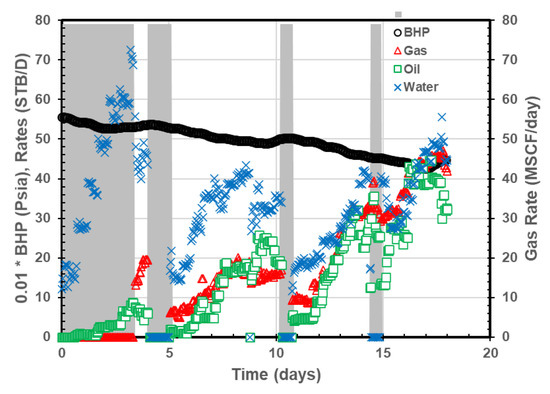
Figure 2.
Field data gathered during the flowback period of the studied MFHW. The gray zones highlight inconsistencies in the data. No gas production is reported for the first zone. In the second through fourth zones, trends in BHP are not consistent with production or lack of production.
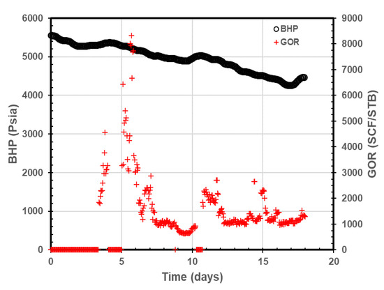
Figure 3.
Field GOR variation during the flowback period. A significant GOR oscillation during the flowback period makes it difficult to select a constant GOR value for the fluid recombination.
3.2. Numerical Reservoir Simulation Model Input, Initialization and History-Match Results
As noted in the Theory and Methods section, the reservoir model used for flowback data history matching was constructed from a geologic sector model; vertical porosity upscaling from the geologic model was implemented, resulting in 26 vertical layers. Figure 4 provides a 3D view of the porosity model. In the reservoir model, the width of the single stage modeled is 65 m in the X direction (parallel to the lateral), represented by 9 gridblocks. In total, 241 gridblocks (1836 m) are used to represent reservoir extension in the Y direction (parallel to the hydraulic fracture).
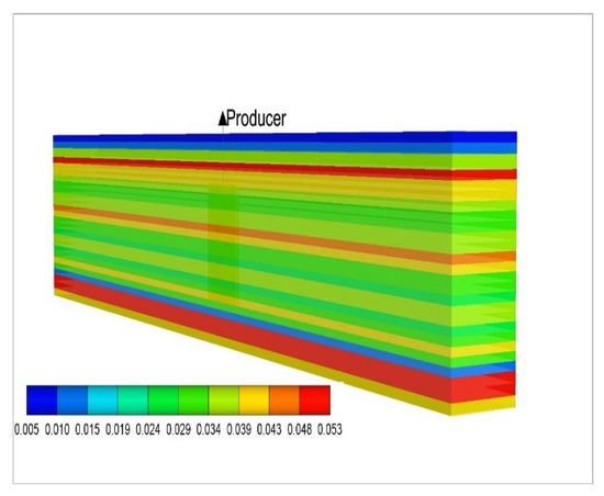
Figure 4.
Three-dimensional view of the porosity model used in this study. The reservoir is divided into 26 horizontal layers, with original values of properties generated in the finer-grid geologic model averaged for each layer.
Figure 5 demonstrates the variation of in situ fluid compositions by vertical layer in the simulated reservoir for a given GOR. Importantly, although the vertical variability in in situ gas composition obtained by combining drill cuttings gas with separator oil is not large (Figure 5), it provided a critical constraint on fracture height growth estimates.
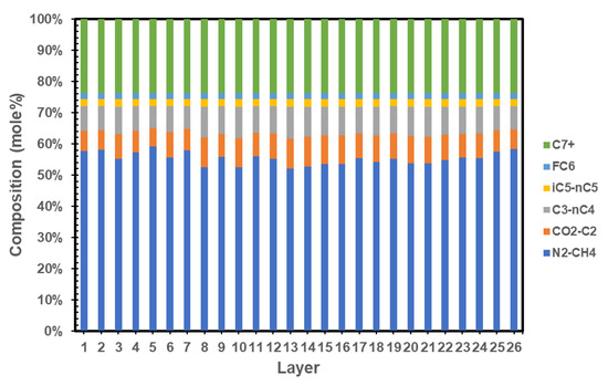
Figure 5.
Fluid composition variation by layer in the reservoir. The top layer in the model is Layer 1. The impact of fluid composition variation with depth on the produced gas composition is controlled by the fracture height extension.
A summary of various model input values used in the simulation is provided in Table 1.

Table 1.
Various model input values.
As noted in the Theory and Methods section, it is important to account for fracture property variation with stress during the flowback period. For this purpose, laboratory propped fracture permeability data as a function of stress was used to generate a HF permeability ratio (permeability at each pressure over the initial permeability value at initial pressure) versus pressure (Figure 6).
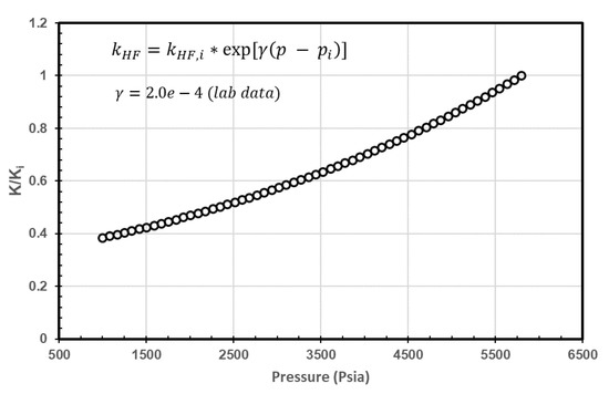
Figure 6.
HF permeability change with pressure. The plot was generated by using stress-dependent propped fracture permeability data measured in the laboratory.
The constructed reservoir model was then used to history match production rates, bottomhole pressures, and compositions of the produced surface gas for the purpose of constraining fracture dimensions. A zero weight factor was applied to uncertain field data during the history match. During the history-matching process, 19 parameters were adjusted to achieve the match and derive HF, SRV, matrix, and fluid properties. Table 2 summarizes the parameters adjusted (and their range) during for the history match.
Table 2.
The list of the parameters (and their ranges) used in history matching with the CMG CMOST simulator.
As noted in the Theory and Methods section, the total hourly fluid production was used as the main simulator constraint, and phase production rates, BHPs, and produced surface gas compositions were matched in order to derive fracture geometry. Figure 7 illustrates how the DE algorithm improves the quality of the history match over several generations by minimizing the global and local errors. The calculated global error decreases and plateaus after 600 runs.
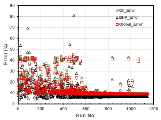
Figure 7.
Calculated history-match global and local errors obtained with the Differential Evolution technique. The decrease in error with run number is demonstrated.
The best-case history-match results are provided in Figure 8. Although the quality of the production rate history match is satisfactory for the entire flowback period, the difference between measured and predicted BHPs becomes quite significant for three distinct time intervals. The simulation predicts a sharp increase in pressure during the two shut-in periods (corresponding to zero production rates). However, the recorded data exhibit a gradual increase in pressure long before the shut-in periods without any associated impact on the production rates. This inconsistency in the recorded data is the primary reason for the low-quality match with BHP pressure prior to the shut-in intervals. The difference between the measured and predicted gas rate data at early time is due to the lack of measured gas data during this period.
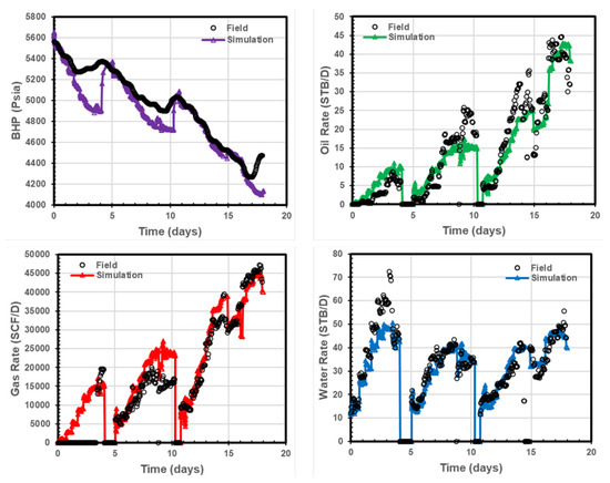
Figure 8.
Results of the best-case history-match results. A good match of water, oil and gas production rates was obtained. Bottomhole pressure was reasonably matched except for the time periods before the well shut-ins.
The reservoir-simulator-predicted surface gas compositions are plotted against sample gas compositions measured at day 17 of the flowback period in Figure 9. A reasonably good match with the field data was achieved. As noted above and observed in Figure 5, the in situ fluid composition varies with depth in the reservoir, as quantified using the isojar samples. Therefore, the produced surface gas composition is controlled by the layers in contact with the hydraulic fractures. The history match resulted in an estimate of upward fracture growth from the well of 65 m (210 ft), and downward growth of 95 m (310 ft). The 40% upward growth in the fracture is consistent with microseismic observations obtained for this well. The best-case match-derived reservoir parameters are reported in Table 3.
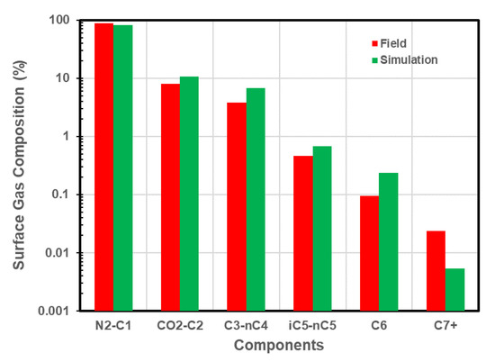
Figure 9.
Surface gas compositions: field vs. simulation model prediction. A reasonable match of the field data was achieved.
Table 3.
Reservoir properties derived from the best-case simulation numerical model history match.
A global sensitivity analysis was also implemented for this study to understand the impact of several parameters on reservoir performance and the quality of the history match. As is apparent from Figure 10, among all of the history match parameters considered in this study, fracture geometry (height and length) was identified as the primary factor influencing the quality of the history match.
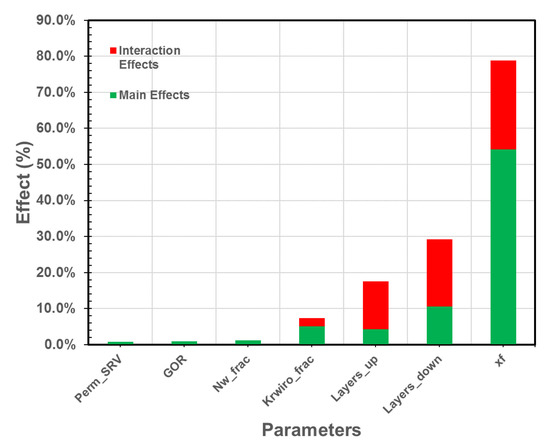
Figure 10.
Results of the global sensitivity analysis. Fracture half-length is the dominant (1st ranked) parameter, while the number of layers above and below the well are 2nd and 3rd, respectively, in the ranking.
3.3. Semi-Analytical DDA Model Individual-Stage Forecast Results
The fracture dimensions, reservoir volume, and fluid properties derived from the numerical model history match in the previous section were then used to constrain the semi-analytical DDA model for forecasting individual-stage production for the subject well. The parameters that were fixed in the modeling are provided in Table 4. Prior to running these predictions, the DDA model was tuned by adjusting the productivity index to ensure it generates the same production profile as that predicted by the history-matched numerical simulator.
Table 4.
Fixed reservoir and fluid properties used for semi-analytical model forecasting runs.
The first step in the analysis was to investigate the sensitivity of the stage forecasts (generated with the DDA model) to reservoir quality determined from the Part 1 study [22]. For this purpose, 15 stages with variable RC/CQ were selected (Table 5). The stage-length-average porosity, permeability, and water saturation, determined using the along-well characterization methods from Part 1, are reported. Figure 11 provides the location of these selected stages along the subject well lateral, as well as an illustration of the along-well variability in permeability, porosity and water saturation derived from the Part 1 study.
Table 5.
Reservoir properties for 15 selected stages. Permeability and water saturations were calculated using the equations of Wood [47], which are based on empirical relationships derived from core and log data from the Montney Formation.
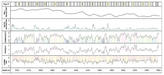
Figure 11.
Location of the 15 selected stages along the horizontal well. Well trajectory, permeability/porosity/water saturation derived from the Part 1 study, and the gamma ray log are also provided.
In Table 6, the selected stages are ranked from 1–15 based on permeability (highest to lowest), porosity (highest to lowest), and water saturation (lowest to highest).
Table 6.
Permeability, porosity, and initial water saturation-based ranking for the selected stages.
From the ranking provided in Table 6, it is observed that Stages 12, 37, and 15 are the top 3 stages for all properties evaluated. Stages 18 and 33 are the bottom two stages in terms of the properties evaluated.
In order to forecast production for each of these 15 stages with the semi-analytical DDA model, the fracture geometry (half-length and height), reservoir volume, and fluid properties obtained from the numerical simulation model history match (Table 4) were input into the model along with the petrophysical properties provided in Table 6. The flowing bottomhole pressure was then set as 3900 psi for 150 days to generate the production forecast; this BHP was set slightly above bubble point pressure because the semi-analytical model is currently capable of forecasting undersaturated oil cases only. Each stage forecast required 1–5 min to run in the DDA model.
The results of these individual stage forecasts are provided in Figure 12, Figure 13, Figure 14 and Figure 15. Figure 12 and Figure 13 provide the oil rate forecasts for the entire forecast period and from 60 to 120 days, respectively, and Figure 14 and Figure 15 provide the water rate forecasts for the entire forecast period, and from 60 to 120 days, respectively. From the results provided, it is evident that there is substantial variability in oil and water production. Certain stages will likely payout the completion/stimulation costs associated with that stage, while others will not; for example, stages 18 and 33 have negligible oil production and possibly will not payout completion/stimulation costs. In terms of the relationship between stage performance and petrophysical properties for each stage (Table 6), it is observed that oil production of each stage is largely consistent with the petrophysical ranking in Table 6. For example, Stage 12 has the highest oil production, and also the highest petrophysical property ranking in Table 6. Stages 9, 37 and 15 have similar oil production, which is also consistent with their similar petrophysical properties and ranking. Stages 18 and 33 have the poorest stage performance, also consistent with their petrophysical ranking. Focusing on water production rates, it is observed that highest oil producing stages also produce the most water; this is because the permeability and porosity of these stages are higher, which offsets their lower water saturation and water relative permeability.
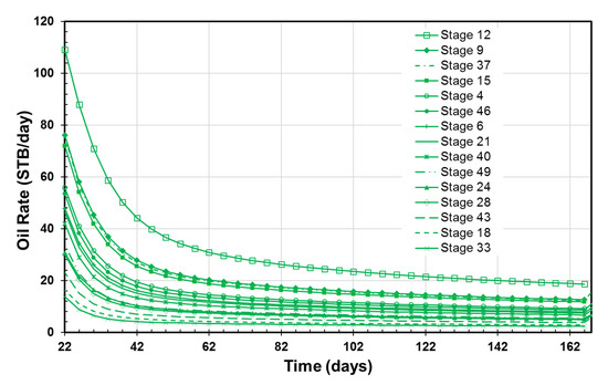
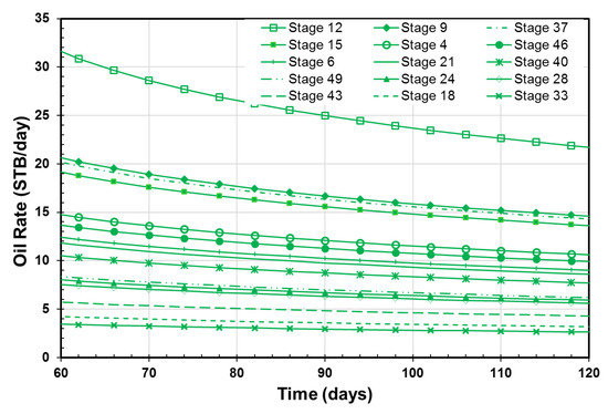
Figure 13.
Same as Figure 12, with a focus on the 60 to 120 days of production.
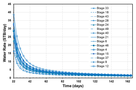
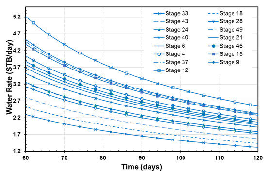
Figure 15.
Same as Figure 14, with a focus on the 60–120 days of production.
Focusing now on the production forecast for all 50 stages of the subject well, petrophysical parameters (permeability, porosity and water saturation) derived for each stage as a result of the Part 1 study were input into the semi-analytical DDA model (along with fracture dimensions, fluid properties and reservoir volume derived from the numerical model history match), and a constant BHP (=3900 psi) was used to generate a 150-day forecast for each stage of the well. The results are presented in terms of the cumulative oil production at the end of the 150-day forecast in Figure 16. A substantial variability in per-stage oil production is exhibited, with several stages producing < 1000 STB of oil during the 150-day period. These results suggest that selective completion of the higher-performing stages may not have substantially impacted the well performance as a whole. This point is explored further in the Discussion section.
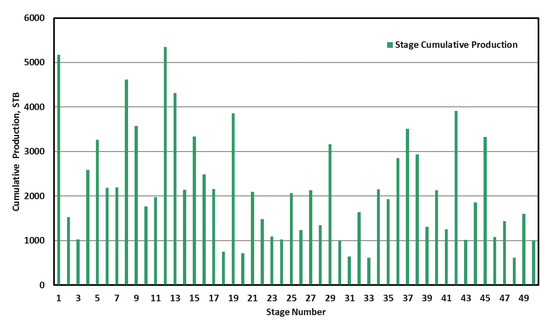
Figure 16.
Cumulative oil production for each stage along the lateral at the end of the 150-day forecast using the DDA model.
4. Discussion
The goal of this two-part study is to demonstrate that rigorous methods to evaluate along-well variability in reservoir/completion quality (Part 1), combined with a simple-yet-rigorous method for predicting stage-by-stage performance that accounts for this variability in reservoir quality (Part 2), may be used to reduce the number of stages completed in a well (through selective stimulation) without a significant sacrifice in well performance. While the previous section demonstrated that production performance of each stage predicted with the DDA model varied substantially along the well (Figure 16), this section explores the impact that selective stage completion could have on total well performance. For this purpose, the per-stage cumulative production was sorted, and then the total cumulative production in sequence from the most productive zone to the least productive zone was calculated (Figure 17). This analysis demonstrates that 60% of the stages (top 30 stages in Figure 17) are able to generate 80% of the total production (if all 50 stages were completed) at the end of the 150-day forecast period, while 74% of the stages (top 37 stages in Figure 17) are able to generate 90% of the production (if all 50 stages were completed). As a result, it may be possible to substantially reduce the stage count (from 50 to 30, or 37), and still retain a large percentage the total well production if all 50 stages were completed. Economic analysis will have to be performed to determine what the optimal stage count reduction will be (benefits of reduced cost are offset by reduced oil production).
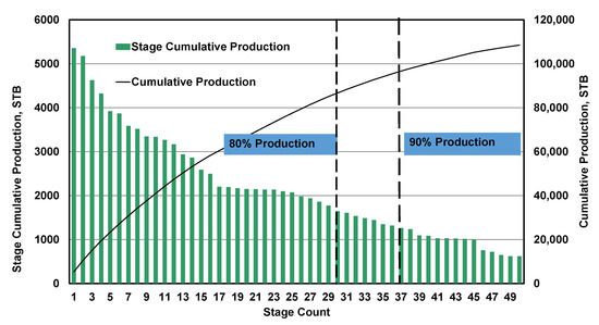
Figure 17.
Plot of per-stage cumulative production, from most productive to least productive, along with total well cumulative production. The top 30 stages (60%) produce 80% of total production. The top 37 stages (74%) produce 90% of the production.
The per-stage forecasting performed using the semi-analytical DDA model in this proof-of-concept has not considered the impact of variable hydraulic fracture properties that may result from variability in geomechanical and reservoir properties. For this study, the fracture dimensions were fixed using the results of the single-stage numerical model history match. However, as noted previously, the DDA model of Zhang et al. [23] included a hydraulic fracture model for predicting hydraulic fracture length and proppant concentration. In future work, the frac-through-flowback DDA model developed by Zhang et al. [23] will be used to predict fracture properties (given stimulation treatment data) prior to generating the per-stage production forecasts. In this way, the per-stage geomechanical properties (Poisson’s ratio and Young’s modulus) can be honored and used to determine the impact on per-stage fracture properties. For reference, Table 7 provides the geomechanical properties (derived from the Part 1 study) for the 15 stages selected for forecasting in the Results section.
Table 7.
Geomechanical properties for 15 selected stages.
5. Conclusions
In this study, a rigorous approach for forecasting production from individual stages in a MFHW completed in a low-permeability, liquids-rich reservoir in the Montney Formation is demonstrated. A compositional numerical simulation model history match of the subject well flowback data is first performed in order to estimate hydraulic fracture extent. Importantly, the combination of estimated in situ fluid compositions with depth in the reservoir, and produced surface gas compositions, are used to constrain fracture height growth in the model.
Given fracture parameters, reservoir volume, and fluid properties derived from the numerical model history match, and along-well petrophysical properties, a semi-analytical model is used to forecast per-stage production. As a starting point, 15 stages with variable petrophysical properties (permeability, porosity, water saturation), were selected for forecasting. The forecasted per-stage oil and water production variability is substantial, with the production variability reflecting the range in petrophysical properties input for each stage. Importantly, it is demonstrated that, by selecting only the highest quality stages in the well for stimulation (as determined from along-well estimates of petrophysical parameters), the stage count can be significantly reduced without a substantial loss in well production (when all stages are completed).
The following are the key findings of this study:
- Fracture dimension has the greatest impact on the numerical model history matching results;
- Fracture height growth constrained by in situ fluid compositions and produced gas compositions is consistent with microseismic observations;
- Per-stage production forecasts generated with the semi-analytical model exhibit substantial variability, reflecting the individual stage petrophysical properties;
- Using the individual-stage forecasts generated for all 50 stages of the subject well, the following can be concluded:
- The top 30 stages (60% of the total number of stages) produce 80% of the total well production (when all 50 stages are completed);
- The top 37 stages (74%) produce 90% of the total well production;
- It is possible to complete fewer stages without a substantial loss in production.
The results of this study have important implications for operators looking to reduce well cost, and lower the environmental impact of their operations, without a substantial loss in well production.
Author Contributions
Conceptualization, C.R.C.; methodology, C.R.C., Z.Z., F.T. and D.B.; program, Z.Z.; formal analysis, Z.Z. and F.T.; data curation, D.B. and A.G.; writing—original draft preparation, C.R.C., Z.Z., F.T. and D.B.; raw data collection, D.B. and A.G.; writing—review and editing, C.R.C., Z.Z., F.T., D.B. and A.G.; supervision, C.R.C.; project administration, C.R.C.; funding acquisition, C.R.C. All authors have read and agreed to the published version of the manuscript.
Funding
This research was funded by NSERC Collaborative Research and Development Grant, grant number CRDPJ 500014-2016.
Acknowledgments
Chris Clarkson would like to acknowledge Ovintiv and Shell for support of his Chair position in Unconventional Gas and Light Oil research at the University of Calgary, Department of Geoscience. The authors would like to thank the sponsors of the Tight Oil Consortium, hosted at the University of Calgary, for their support.
Conflicts of Interest
The authors declare no conflict of interest.
Nomenclature
| total matrix surface area in a dynamic drainage area, ft2 | |
| oil formation volume factor, RB/STB | |
| initial oil formation volume factor, RB/STB | |
| water formation volume factor, RB/STB | |
| initial water formation volume factor, RB/STB | |
| total initial primary hydraulic fracture compressibility, 1/psi | |
| total matrix compressibility, 1/psi | |
| hydraulic fracture height, m or ft | |
| GOR | gas-to-oil ratio, scf/STB |
| Krg (HF) | Brooks-Corey gas relative permeability end point in hydraulic fracture |
| Krgl (HF) | Brooks-Corey liquid relative permeability end point in hydraulic fracture |
| Krow (HF) | Brooks-Corey oil relative permeability end point in hydraulic fracture |
| Krw (HF) | Brooks-Corey water relative permeability end point in hydraulic fracture, dimensionless |
| Krw (HF) | Brooks-Corey water relative permeability end point in hydraulic fracture, dimensionless |
| primary hydraulic fracture permeability, md | |
| initial primary hydraulic fracture permeability, md | |
| initial matrix permeability, md | |
| primary hydraulic fracture primary-phase relative permeability, dimensionless | |
| matrix primary-phase relative permeability, dimensionless | |
| matrix oil relative permeability, dimensionless | |
| primary hydraulic fracture water relative permeability, dimensionless | |
| matrix water relative permeability, dimensionless | |
| primary hydraulic fracture oil normalized pseudopressure, psia | |
| matrix oil normalized pseudopressure, psia | |
| primary hydraulic fracture water normalized pseudopressure, psia | |
| matrix water normalized pseudopressure, psia | |
| cumulative oil transfer amount between the fracture and matrix, STB | |
| cumulative oil production, STB | |
| number of simulation grids in x direction | |
| Brooks-Corey gas exponent term in hydraulic fracture, dimensionless | |
| number of fracture stages | |
| Brooks-Corey oil-gas exponent term in hydraulic fracture, dimensionless | |
| Brooks-Corey oil-water exponent term in hydraulic fracture, dimensionless | |
| Brooks-Corey water exponent term in hydraulic fracture, dimensionless | |
| number of fracture stages | |
| reservoir pressure, psia | |
| average primary hydraulic fracture pressure in distance of investigation, psia | |
| average matrix pressure in distance of investigation, psia | |
| bottomhole pressure, psia | |
| oil production rate from primary hydraulic fracture, STB/day | |
| oil transfer rate between the fracture and matrix, STB/day | |
| water production rate from primary hydraulic fracture, STB/day | |
| water transfer rate between fracture and matrix, STB/day | |
| Brooks-Corey critical gas saturation term in hydraulic fracture, dimensionless | |
| initial primary hydraulic fracture oil saturation, dimensionless | |
| initial matrix oil saturation, dimensionless | |
| Brooks-Corey residual oi saturation to gas in hydraulic fracture, dimensionless | |
| Brooks-Corey residual oi saturation to water in hydraulic fracture, dimensionless | |
| Brooks-Corey connate water saturation term in hydraulic fracture, dimensionless | |
| initial primary hydraulic fracture water saturation, dimensionless | |
| initial water saturation, dimensionless | |
| initial matrix water saturation, dimensionless | |
| Brooks-Corey residual oil saturation term in hydraulic fracture, dimensionless | |
| primary hydraulic fracture oil saturation in distance of investigation, dimensionless | |
| matrix oil saturation in distance of investigation, dimensionless | |
| primary hydraulic fracture water saturation in distance of investigation, dimensionless | |
| matrix water saturation in distance of investigation, dimensionless | |
| reservoir temperature, °F | |
| time, s or day | |
| cumulative water transfer amount between the fracture and matrix, STB | |
| cumulative water production, STB | |
| the average width of primary hydraulic fracture or unpropped fracture width, ft | |
| fracture half length, ft | |
| the distance of investigation in fracture, ft | |
| maximum matrix distance perpendicular to primary hydraulic fracture into the reservoir, ft | |
| the distance of investigation in matrix, ft | |
| time step, days | |
| distance of investigation coefficient, dimensionless | |
| initial primary-phase viscosity, cp | |
| oil viscosity, cp | |
| initial oil viscosity, cp | |
| water viscosity, cp | |
| initial water viscosity, cp | |
| primary hydraulic fracture porosity, dimensionless | |
| initial primary hydraulic fracture porosity, dimensionless | |
| initial matrix porosity, dimensionless | |
| matrix porosity, dimensionless |
References
- Baihly, J.D.; Malpani, R.; Edwards, C.; Han, S.Y.; Kok, J.C.; Tollefsen, E.M.; Wheeler, C.W. Unlocking the shale mystery: How lateral measurements and well placement impact completions and resultant production. In Proceedings of the Tight Gas Completions Conference, San Antonio, TX, USA, 2 November 2010. [Google Scholar] [CrossRef]
- Miller, C.; Waters, G.; Rylander, E. Evaluation of production log data from horizontal wells drilled in organic shales. In Proceedings of the North American Unconventional Gas Conference and Exhibition, The Woodlands, TX, USA, 14 June 2011. [Google Scholar] [CrossRef]
- Duong, A.N. Rate-Decline Analysis for Fracture-Dominated Shale Reservoirs. SPE Reserv. Eval. Eng. 2011, 14, 377–387. [Google Scholar] [CrossRef] [Green Version]
- Ilk, D.; Perego, A.D.; Rushing, J.A.; Blasingame, T.A. Integrating multiple production analysis techniques to assess tight gas sand reserves: Defining a new paradigm for industry best practices. In Proceedings fo the CIPC/SPE Gas Technology Symposium 2008 Joint Conference, Calgary, AB, Canada, 16 June 2008. [Google Scholar] [CrossRef]
- Ilk, D.; Rushing, J.A.; Perego, A.D.; Blasingame, T.A. Exponential vs. hyperbolic decline in tight gas sands: Understanding the origin and implications for reserve estimates using arps’ decline curves. SPE Annu. Tech. Conf. Exhib. 2008, 23. [Google Scholar] [CrossRef]
- Valko, P.P.; Lee, W.J. A better way to forecast production from unconventional gas wells. SPE Annu. Tech. Conf. Exhib. 2010, 16. [Google Scholar] [CrossRef]
- Brown, M.; Ozkan, E.; Raghavan, R.; Kazemi, H. Practical Solutions for pressure-transient responses of fractured horizontal wells in unconventional shale reservoirs. SPE Reserv. Eval. Eng. 2011, 14, 663–676. [Google Scholar] [CrossRef]
- Ozkan, E.; Brown, M.; Raghavan, R.; Kazemi, H. Comparison of fractured-horizontal-well performance in tight sand and shale reservoirs. SPE Reserv. Eval. Eng. 2011, 14, 248–259. [Google Scholar] [CrossRef]
- Apaydin, O.G.G.; Ozkan, E.; Raghavan, R. Effect of discontinuous microfractures on ultratight matrix permeability of a dual-porosity medium. SPE Reserv. Eval. Eng. 2012, 15, 473–485. [Google Scholar] [CrossRef]
- Stalgorova, E.; Mattar, L. Practical analytical model to simulate production of horizontal wells with branch fractures. In Proceedings of the SPE Canada Unconventional Resources Conference, Pittsburgh, PA, USA, 5–7 June 2021. SPE 162515. [Google Scholar] [CrossRef]
- Stalgorova, K.; Mattar, L. Analytical model for unconventional multifractured composite systems. SPE Reserv. Eval. Eng. 2013, 16, 246–256. [Google Scholar] [CrossRef]
- Clarkson, C.R.; Qanbari, F.; Williams-Kovacs, J.D. Semi-analytical model for matching flowback and early-time production of multi-fractured horizontal tight oil wells. J. Unconv. Oil Gas Resour. 2016, 15, 134–145. [Google Scholar] [CrossRef]
- Nobakht, M.; Mattar, L.; Moghadam, S.; Anderson, D.M. Simplified forecasting of tight/shale-gas production in linear flow. J. Can. Pet. Technol. 2012, 51, 476–486. [Google Scholar] [CrossRef]
- Nobakht, M.; Ambrose, R.; Clarkson, C.R.; Youngblood, J.E.; Adams, R. Effect of completion heterogeneity in a horizontal well with multiple fractures on the long-term forecast in shale-gas reservoirs. J. Can. Pet. Technol. 2013, 52, 417–425. [Google Scholar] [CrossRef]
- Clarkson, C.R.; Qanbari, F. History matching and forecasting tight gas condensate and oil wells by use of an approximate semianalytical model derived from the dynamic-drainage-area concept. SPE Reserv. Eval. Eng. 2016, 19, 540–552. [Google Scholar] [CrossRef]
- Ajisafe, F.; Pope, T.; Azike, O.; Reischman, R.; Herman, D.; Burkhardt, C.; Helmreich, A.; Phelps, M. Engineered completion workflow increases reservoir contact and production in the Wolfcamp Shale, West Texas. In Proceedings of the SPE Annual Technical Conference and Exhibition, Amsterdam, The Netherlands, 27 October 2014. [Google Scholar]
- Stolyarov, S.; Roberts, K.; Sadykhov, S.; Rebol, A.; Vinh, C. Less money for more oil-Advanced Drill Cuttings Analysis Improves Post Fracture Oil Production, Wolfcamp Example. In Proceedings of the Abu Dhabi International Petroleum Exhibition & Conference, Abu Dhabi, UAE, 7 November 2016. [Google Scholar] [CrossRef]
- Stolyarov, S.; Gadzhimirzaev, D.; Sadykhov, S.; Ackley, B.; Lipp, C. Lateral wellbore rock characterization and hydraulic fracture optimization utilizing drilling cuttings and mud log in Cleveland Sand: A case study. In Proceedings of the SPE Oklahoma City Oil and Gas Symposium, Oklahoma City, OK, USA, 27 March 2017. [Google Scholar] [CrossRef]
- Logan, W.D. Engineered shale completions based on common drilling data. In Proceedings of the SPE Annual Technical Conference and Exhibition, Houston, TX, USA, 28 September 2015. [Google Scholar] [CrossRef]
- Yang, J.; Stolyarov, S.; Cazeneuve, E.; Simmons, J.; Kotov, S.; Gadzhimizaev, D. An integrated analytics platform for completion optimization and reservoir characterization. In Proceedings of the SPE International Hydraulic Fracturing Technology Conference and Exhibition, Muscat, Oman, 16 October 2018. [Google Scholar] [CrossRef]
- Cipolla, C.; Weng, X.; Onda, H.; Nadaraja, T.; Ganguly, U.; Malpani, R. New Algorithms and Integrated Workflow for Tight Gas and Shale Completions. In Proceedings of the SPE Annual Technical Conference and Exhibition, Denver, CO, USA, 30 October 2011. [Google Scholar] [CrossRef]
- Becerra, D.; Clarkson, C.R.; Ghanizadeh, A.; Pires de Lima, R.; Tabasinejad, F.; Zhang, Z.; Trivedi, A.; Shor, R. Evaluation of reservoir quality and forecasted production variability along a multi-fractured horizontal well. part 1: Reservoir characterization. Energies 2021. [Google Scholar]
- Zhang, Z.; Clarkson, C.; Williams-Kovacs, J.D.; Yuan, B.; Ghanizadeh, A. Rigorous estimation of the initial conditions of flowback using a coupled hydraulic-fracture/dynamic-drainage-area leakoff model constrained by laboratory geomechanical data. SPE J. 2020, 25, 3051–3078. [Google Scholar] [CrossRef]
- Clarkson, C.R.; Ghaderi, S.M.; Kanfar, M.S.; Iwuoha, C.S.; Pedersen, P.K.; Nightingale, M.; Shevalier, M.; Mayer, B. Estimation of fracture height growth in layered tight/shale gas reservoirs using flowback gas rates and compositions–Part II: Field application in a liquid-rich tight reservoir. J. Nat. Gas Sci. Eng. 2016, 36, 1031–1049. [Google Scholar] [CrossRef]
- Ghanizadeh, A.; Clarkson, C.R.; Aquino, S.; Ardakani, O.H.; Sanei, H. Petrophysical and geomechanical characteristics of Canadian tight oil and liquid-rich gas reservoirs: I. Pore network and permeability characterization. Fuel 2015, 153, 664–681. [Google Scholar] [CrossRef]
- Clarkson, C.R.; Jensen, J.L.; Pedersen, P.K.; Freeman, M. Innovative methods for flow-unit and pore-structure analyses in a tight siltstone and shale gas reservoir. Am. Assoc. Pet. Geol. Bull. 2012, 96, 355–374. [Google Scholar]
- Hamdi, H.; Behmanesh, H.; Clarkson, C.R.; Sousa, M.C. Using differential evolution for compositional history-matching of a tight gas condensate well in the Montney Formation in western Canada. J. Nat. Gas Sci. Eng. 2015, 26, 1317–1331. [Google Scholar] [CrossRef]
- Ahmadi, H.; Clarkson, C.R.; Hamdi, H.; Behmanesh, H. Analysis of production data from communicating multifractured horizontal wells using the dynamic drainage area concept. SPE Reserv. Eval. Eng. 2021, 1–19. [Google Scholar] [CrossRef]
- McCain, W.D., Jr. The Properties of Petroleum Fluids, 2nd ed.; PennWell Corporation: Neshvili, TN, USA, 1990. [Google Scholar]
- Ghanizadeh, A.; Clarkson, C.R.; Deglint, H.; Vahedian, A.; Aquino, S.; Wood, J.M. Unpropped/Propped Fracture Permeability and Proppant Embedment Evaluation: A Rigorous Core-Analysis/Imaging Methodology. In Proceedings of the Unconventional Resources Technology Conference, San Antonio, TX, USA, 1–3 August 2016. URTEC-2459818-MS. [Google Scholar] [CrossRef]
- Forchheimer, P. Wasserbewegung durch boden. Z. Des. Vereines Dutsch Ingenieure 1901, 45, 339–355. [Google Scholar]
- Brooks, R.H.; Corey, A.T. Hydraulic Properties of Porous Media. Hydrol. Pap. 1964, 27, 37. [Google Scholar]
- Aziz, K.; Settari, A. Petroleum Reservoir Simulation; Blitzprint Inc.: Calgary, AB, Canada, 2002. [Google Scholar]
- CMG. CMOST-AI User’s Guide: Intelligent Optimization and Analysis Tool; Computer Modelling Group Ltd.: Calgary, AB, Canada, 2018. [Google Scholar]
- Storn, R.; Price, K. Differential evolution–A simple and efficient heuristic for global optimization over continuous spaces. J. Glob. Optim. 1997, 11, 341–359. [Google Scholar] [CrossRef]
- Decker, J.; Mauldon, M. Determining size and shape of fractures from trace data using a differential evolution algorithm. In Proceedings of the 41st U.S. Symposium on Rock Mechanics (USRMS), Golden, CO, USA, 17 June 2006. ARMA-06-969. [Google Scholar]
- Hajizadeh, Y.; Christie, M.A.; Demyanov, V. Application of Differential Evolution as a New Method for Automatic History Matching. In Porceedings of the Kuwait International Petroleum Conference and Exhibition, Kuwait City, Kuwait, 14 December 2009; SPE-127251-MS. 1272. [Google Scholar] [CrossRef]
- Mirzabozorg, A.; Nghiem, L.; Chen, Z.; Yang, C. Differential evolution for assisted history matching process: SAGD case study. In Proceedings of the SPE Heavy Oil Conference-Canada, Calgary, AB, Canada, 11 June 2013. SPE-165491-MS. [Google Scholar] [CrossRef]
- Awotunde, A.A.; Mutasiem, M.A. Efficient drilling time optimization with differential evolution. In Proceedings of the SPE Nigeria Annual International Conference and Exhibition, Lagos, Nigeria, 5 August 2014. SPE-172419-MS. [Google Scholar] [CrossRef]
- Ma, X.; Zhang, K.; Zhang, L.; Yao, C.; Yao, J.; Wang, H.; Jian, W.; Yan, Y. Data-driven niching differential evolution with adaptive parameters control for history matching and uncertainty quantification. SPE J. 2021, 26, 993–1010. [Google Scholar] [CrossRef]
- Hatchell, P.; Tatanova, M. 4D seismic data matching using spectrum balancing filters. In Proceedings of the 81st EAGE Conference and Exhibition 2019, London, UK, 3–6 June 2019; pp. 1–5. [Google Scholar] [CrossRef]
- Price, K.; Storn, R.M.; Lampinen, J. Differential Evolution: A Practical Approach to Global Optimization; Springer: Basel, Switzerland, 2005. [Google Scholar]
- Clarkson, C.R.; Qanbari, F.; Williams-Kovacs, J.D.; Zanganeh, B. Fracture Propagation, Leakoff and Flowback Modeling for Tight Oil Wells Using the Dynamic Drainage Area Concept. In Proceedings of the SPE Western Regional Meeting, Bakersfield, CA, USA, 23 April 2017. [Google Scholar] [CrossRef]
- Shahamat, M.S.; Mattar, L.; Aguilera, R. A Physics-Based Method To Forecast Production From Tight and Shale Petroleum Reservoirs by Use of Succession of Pseudosteady States. SPE Reserv. Eval. Eng. 2015, 18, 508–522. [Google Scholar] [CrossRef]
- Clarkson, C.R.; Williams-Kovacs, J.D. Flowback and Early-Time Production Data Analysis. In Hydraulic Fracturing: Fundamentals and Advancements; Miskimins, J., Ed.; Society of Petroleum Engineers: Richardson, TX, USA, 2019; p. 795. ISBN 978-1-61399-719-2. [Google Scholar]
- Behmanesh, H.; Clarkson, C.R.; Tabatabaie, S.H.; Heidari Sureshjani, M. Impact of distance-of-investigation calculations on rate-transient analysis of unconventional gas and light-oil reservoirs: New formulations for linear flow. J. Can. Pet. Technol. 2015, 54, 509–519. [Google Scholar] [CrossRef]
- Wood, J.M.M. Water distribution in the montney tight gas play of the Western Canadian sedimentary basin: Significance for resource evaluation. SPE Reserv. Eval. Eng. 2013, 16, 290–302. [Google Scholar] [CrossRef]
Publisher’s Note: MDPI stays neutral with regard to jurisdictional claims in published maps and institutional affiliations. |
© 2021 by the authors. Licensee MDPI, Basel, Switzerland. This article is an open access article distributed under the terms and conditions of the Creative Commons Attribution (CC BY) license (https://creativecommons.org/licenses/by/4.0/).