Thermographic Measurement of the Temperature of Reactive Power Compensation Capacitors

Abstract

An excessive increase in reactive power consumption is unfavorable from the point of view of a power system. For this reason, devices compensating reactive power consumption are used. The capacitor is one such device. Capacitors must be tested regularly during their exploitation. One of the activities that should be performed is testing the degree of heating of the cells of a capacitor bank. Thermography can be used to perform such tests. This non-contact method has its limitations. Due to the angular emissivity and the change in the distance between the lens and the object under observation, the temperature measured with a thermographic camera may differ from the actual temperature. This phenomenon is visible on cylindrical capacitor cases. Consequently, depending on the location of the observation point on the capacitor case, the result of the thermographic temperature measurement may be different. To investigate this phenomenon, experimental work has been undertaken.

1. Introduction

The operation of electrical devices is related to the power consumption by the power system [1]. In the case of devices powered by alternating current, two components of the consumed power can be distinguished: active power and reactive power. Active power is considered to be useful power [2]. It is a component of power that is used to generate work or heat [3]. On the other hand, reactive power is most often associated with the magnetization of the coils of electrical motors and transformers [4]. The consumption of this power is unfavorable from the point of view of the system, as it reduces the power factor of the system and limits the ability of the generators to deliver useful power [5]. It causes an increase in the value of the consumed electrical current, increasing the load on the supply line [6]. In the case of industrial factories, the consumed reactive power is usually inductive [7].

The consumption of inductive reactive power can be compensated by the consumption of capacitive reactive power [8]. It is possible after adding a device whose operation increases the consumption of capacitive reactive power. The capacitor is such a device [9]. The use of capacitors to compensate the consumption of inductive reactive power is a frequently used solution [10]. Reactive power compensation capacitors must be checked regularly. The regular checking of the capacitors makes it possible to detect their capacity decline below the permissible value, which may be caused by the passage of time [11]. Additionally, it is possible to detect a potential failure before it occurs [12]. One of the activities that should be performed while testing the capacitor bank is checking the degree of heating of individual capacitor cells [13].

A method that allows one to check the degree of heating of the capacitor bank cells is thermography. More and more often, the offers of various manufacturers include inexpensive thermographic cameras with parameters that allow checking the heating of individual capacitor cells. This non-destructive method has been approved by the Polish Office of Technical Inspection [14]. It is worth remembering that capacitors used for compensating reactive power work with voltages, which can be hazardous to human health. For this reason, touching the case of a capacitor with a temperature sensor may cause an electric shock. This problem can be minimized by the use of thermography, which is a non-contact method. Consequently, the use of this method to check the degree of heating of individual capacitor cells increases the safety of the person performing the measurement. The most important factors that influence the result of the thermal imaging measurement of temperature ϑ_t are the values of emission factor ε [15], reflected temperature ϑ_refl [16], distance between the camera lens and the object under observation d [17], ambient temperature ϑ_a [18], external optical system temperature ϑ_l [19], transmission of the external optical system τ_l [20], and relative humidity ω [21]. Their effect on the temperature ϑ_t read from a thermogram has been widely described [22]. Furthermore, these values, if correctly determined, make it possible to minimize their effect on ϑ_t. It can be achieved by selecting appropriate coefficients in the thermographic camera software [23].

An additional factor that influences the value of ϑ_t is the recorded thermogram’s lack of sharpness [24]. Modern thermographic cameras are often equipped with automatic sharpness adjustment systems working similarly to systems used in digital cameras [25]. For this reason, making a thermogram with a satisfactory sharpness is not difficult. It becomes problematic when one uses cameras that do not have such a system.

Another problem that can be encountered during thermographic temperature measurement is the low ε value of the material frequently used to make capacitor cases, i.e., aluminum [26], which has a low value of ε (0.238–0.247) at a spectral range of 8–14 μm [27]. For non-transparent materials, the relationship between ε and the reflection factor ρ can be described by Equation (1) [28].

ε + ρ = 1

(1)

Based on Equation (1), it can be concluded that in the case of aluminum, the value of ρ is high. For this reason, while checking the degree of heating of individual capacitor cells, special attention should be paid to ϑ_refl compensation.

Another issue that can be encountered is the cylindrical shape of the capacitor case. The value of ϑ_t measured on the part of the case in front of the thermographic camera differs from the value of ϑt measured on another part of the case. In order to show this phenomenon, a thermogram of the Pt 1000 temperature sensor with a known temperature of ϑ_s = 49.6 °C was made. The temperature of the sensor was selected arbitrarily. The sensor was placed in a metal case with a diameter of ϕ = 3 mm and a length of l = 6 mm. The recorded thermograms showing the sensor case are presented in Figure 1.

In order to confirm the occurrence of this phenomenon, three additional thermograms were made on the cylindrical case of the capacitor, which showed an electrolytic capacitor with a diameter of ϕ = 4 mm. In this case, the capacitor was painted with Velvet Coating 811-21 with a known value of the emissivity factor ε ranging from 0.970 to 0.975 for temperatures between −36 °C and 82 °C. The uncertainty with which the value of emissivity factor was determined was 0.004 [29]. A layer of the paint was applied to the outer surface of the capacitor. During the making of the thermograms, the capacitor was placed on a heating mat at a temperature of 60 °C. The temperature of the mat was selected arbitrarily so that it differed from the value of ϑ_a. The measurement was taken only after the temperature of the capacitor stabilized. The recorded thermograms are shown in Figure 2.

After recording the thermograms, the following question was asked: how big will the error be in measuring the temperature of the capacitor bank cell if the measuring point is not on the surface exactly in front of the thermographic camera lens? It was noticed that the phenomenon shown in Figure 1 and Figure 2 was due to a different angle of view α and a different distance d between the point on the capacitor case and the lens of the thermographic camera. Due to the low ε value of the capacitor case, the following question was asked: how much influence does the reflected temperature have on the measurement result? Following an analysis of the available literature, information on the influence of d on the value of ϑ_t was found. Information on the influence of the angle of view α on the value of ϑ_t was also found. The conducted analysis of the literature did not provide an answer to the question about the value of the error of the thermographic temperature measurement on the case of the capacitor intended for reactive power compensation due to the influence of d, α and ϑ_refl. For this reason, research has been undertaken, the results of which will make it possible to answer that question.

2. Theory and Measurement Systems

2.1. Observed Phenomena

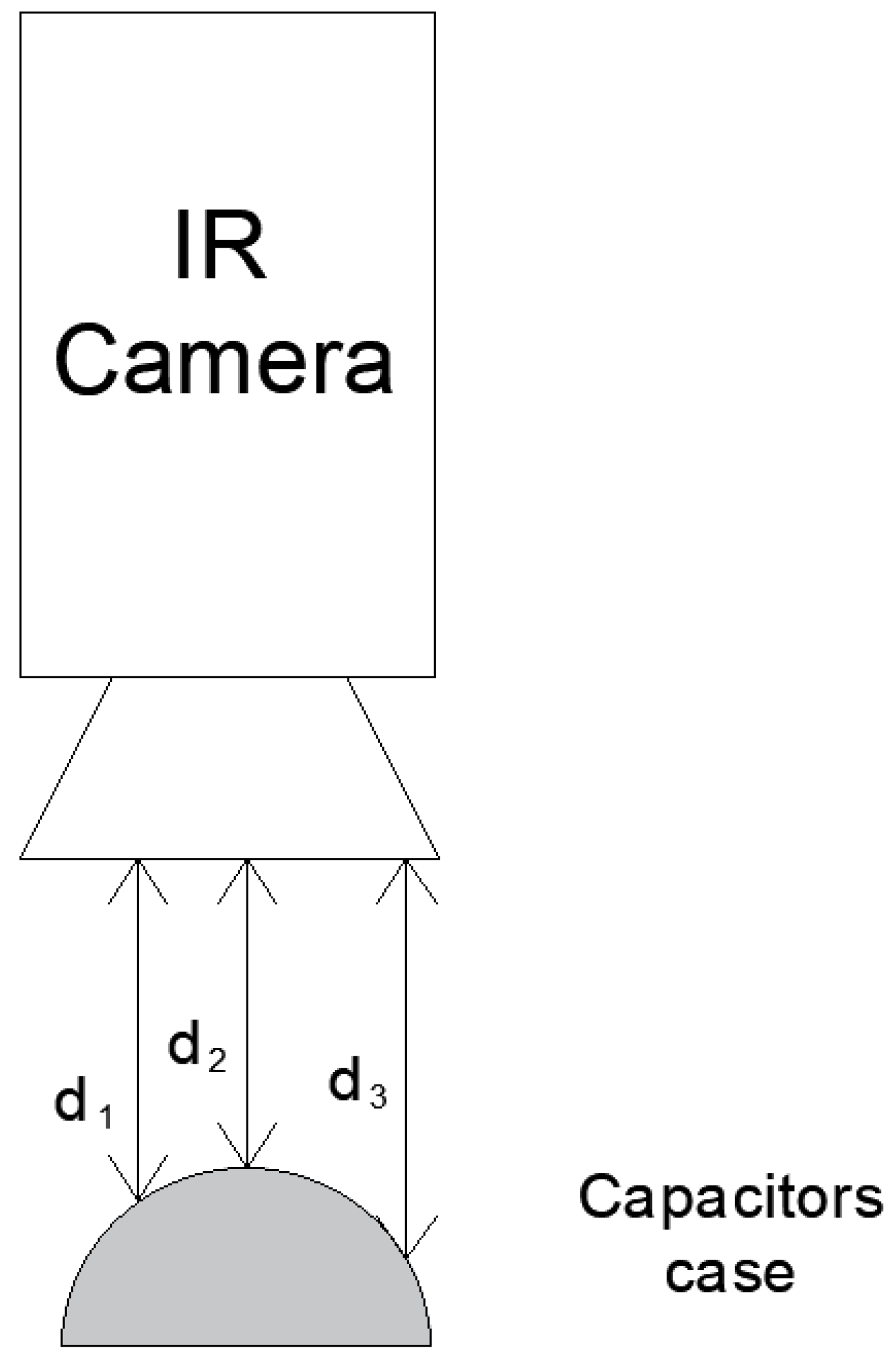
2.1.1. Distance between Thermographic Camera Lens and Observed Object

The phenomenon recorded in Figure 1 and Figure 2 is the result of the occurrence of two phenomena: the change in d and the angular emissivity. The capacitor case has the shape of a cylinder. For this reason, the distances between the lens of the thermographic camera and specific parts of the capacitor case will be different. The damping of the atmosphere layer τ_a between the observed capacitor and the lens of the thermographic camera changes together with the change in d. The relationship between both quantities is described by Equation (2) [29,30]:

$${\tau }_a(d,\omega )=K_a\cdot \exp [-\sqrt{d}\cdot ({\alpha }_1+{\beta }_1\sqrt{\omega }\left)\right]+(1-K_a)\cdot \exp [-\sqrt{d}\cdot ({\alpha }_2+{\beta }_2\sqrt{\omega })]$$

(2)

where K_atm = 1.9 is the atmosphere damping factor, α₁ = 0.0066 and α₂ = 0.0126 are damping factors for an atmosphere without water vapor, β₁ = −0.0023 and β₂ = −0.0067 are damping factors for water vapor, and ω is the factor indicating the amount of water vapor in the atmosphere [29,30].

The value of ω in (2) can be determined using Equation (3) [29,30]:

$$\omega (\omega \%,{\vartheta }_{\mathrm{a}})=\omega \%\cdot \exp (h_1+h_2{\vartheta }_a+h_3{\vartheta }_a^2+h_4{\vartheta }_a^3)$$

(3)

where ω% is the relative humidity: h₁ = 1.5587, h₂ = 6.939 · 10⁻², h₃ = −2.7816 · 10⁻⁴, and h₄ = 6.845 · 10⁻⁷ [30].

It is worth noting that the value of τa is one of the input variables of the equation that allows us to determine the value of ϑ_obj from the total flux of IR radiation reaching the lens of the thermographic camera. The relationship between ϑ_obj and τ_a is described by Equation (4) [31]:

$${\vartheta }_{obj}=\sqrt[4]{\frac{W_{tot}-\left(1-\epsilon \right)\cdot {\tau }_a\cdot \sigma \cdot {\vartheta }_{refl}^4-\left(1-{\tau }_a\right)\cdot \sigma \cdot {\vartheta }_a^4}{\epsilon \cdot \sigma \cdot {\tau }_a}}$$

(4)

where σ is the Boltzmann constant equal to 5.67 cm × 10⁻⁸ W/(m²·K⁴), W_tot is the total IR radiation reaching the camera lens, and τ_a is the atmospheric transmittance [31].

The differences in the d value between the capacitor case and the camera lens are shown in Figure 3.

2.1.2. Angular Emissivity

In order to explain the relationship between ε and α, refer to Equation (1). The ρ factor is the average of the parallel polarized reflectance factor ${\rho }_{\Vert }$ and the perpendicularly polarized reflectance factor ${\rho }_{⟂}$(5) [31]:

$$\rho =\frac{{\rho }_{\Vert }+{\rho }_{⟂}}{2}$$

(5)

The values of ${\rho }_{\Vert }$ and ${\rho }_{⟂}$ depend on the value of α and the refractive factor n. Aluminum, often used to make capacitor cases, is a glossy material, similar to other metals. For glossy materials with damping of the electromagnetic radiation wave, the complex value of the refractive factor n’ = n − jk is assumed, where k is the damping factor. The values of factors ${\rho }_{\Vert }$ and ${\rho }_{⟂}$ can be described by Equations (6) and (7) [31]:

$${\rho }_{\Vert }=\frac{{[n·\cos \left(\alpha \right)-1]}^2+k^2·{\cos }^2\left(\alpha \right)}{{[n·\cos \left(\alpha \right)+1]}^2+k^2·{\cos }^2\left(\alpha \right)}$$

(6)

$${\rho }_{⟂}=[\frac{\sqrt{{\left(\frac{n_2}{n_1}\right)}^2-{\sin }^2\left(\alpha \right)}-\cos \left(\alpha \right)}{\sqrt{{\left(\frac{n_2}{n_1}\right)}^2-{\sin }^2\left(\alpha \right)}+\cos \left(\alpha \right)}]$$

(7)

By inserting Equations (6) and (7) into Equation (5) and then into Equation (1), the relationship between α and ε can be seen.

The outer parts of some capacitors are covered with a thin layer of plastic. In the case of dielectrics, the values of ${\rho }_{\Vert }$ and ${\rho }_{⟂}$ can be described by Equations (8) and (9) [31]:

$${\rho }_{\Vert }=[\frac{{\left(\frac{n_1}{n_2}\right)}^2\cos \left(\alpha \right)-\sqrt{\left(\frac{n_1}{n_2}\right)-{\sin }^2\left(\alpha \right)}}{{\left(\frac{n_2}{n_1}\right)}^2\cos \left(\alpha \right)-\sqrt{\left(\frac{n_2}{n_1}\right)-{\sin }^2\left(\alpha \right)}}]$$

(8)

$${\rho }_{⟂}=[\frac{\sqrt{{\left(\frac{n_2}{n_1}\right)}^2-{\sin }^2\left(\alpha \right)}-\cos \left(\alpha \right)}{\sqrt{{\left(\frac{n_2}{n_1}\right)}^2-{\sin }^2\left(\alpha \right)}+\cos \left(\alpha \right)}]$$

(9)

where n₁ is the refractive factor of the first medium and n₂ is the refractive factor of the second medium.

Based on Equations (6)–(9), it can be concluded that the characteristics ε = f(α) for metals and dielectrics will be different.

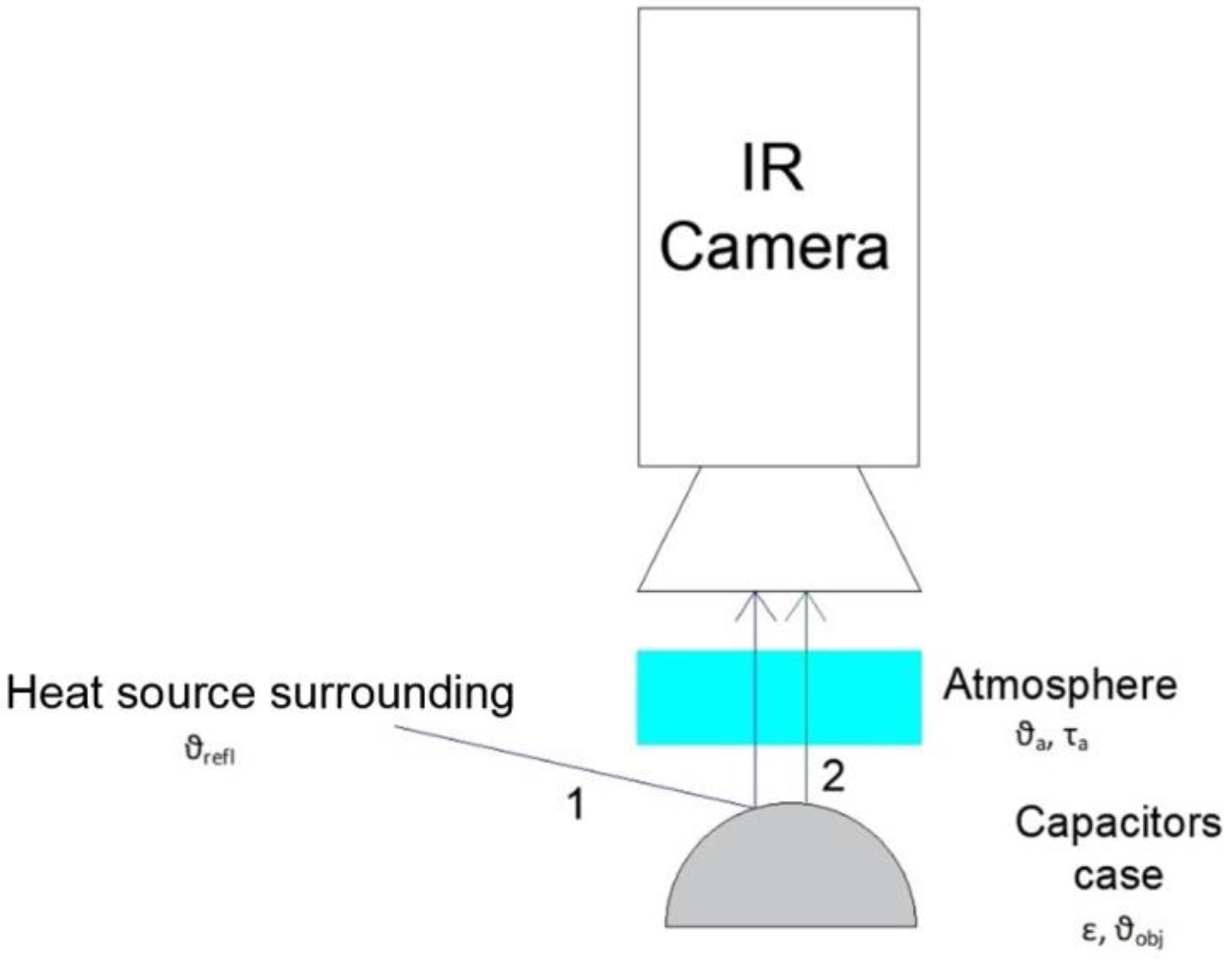
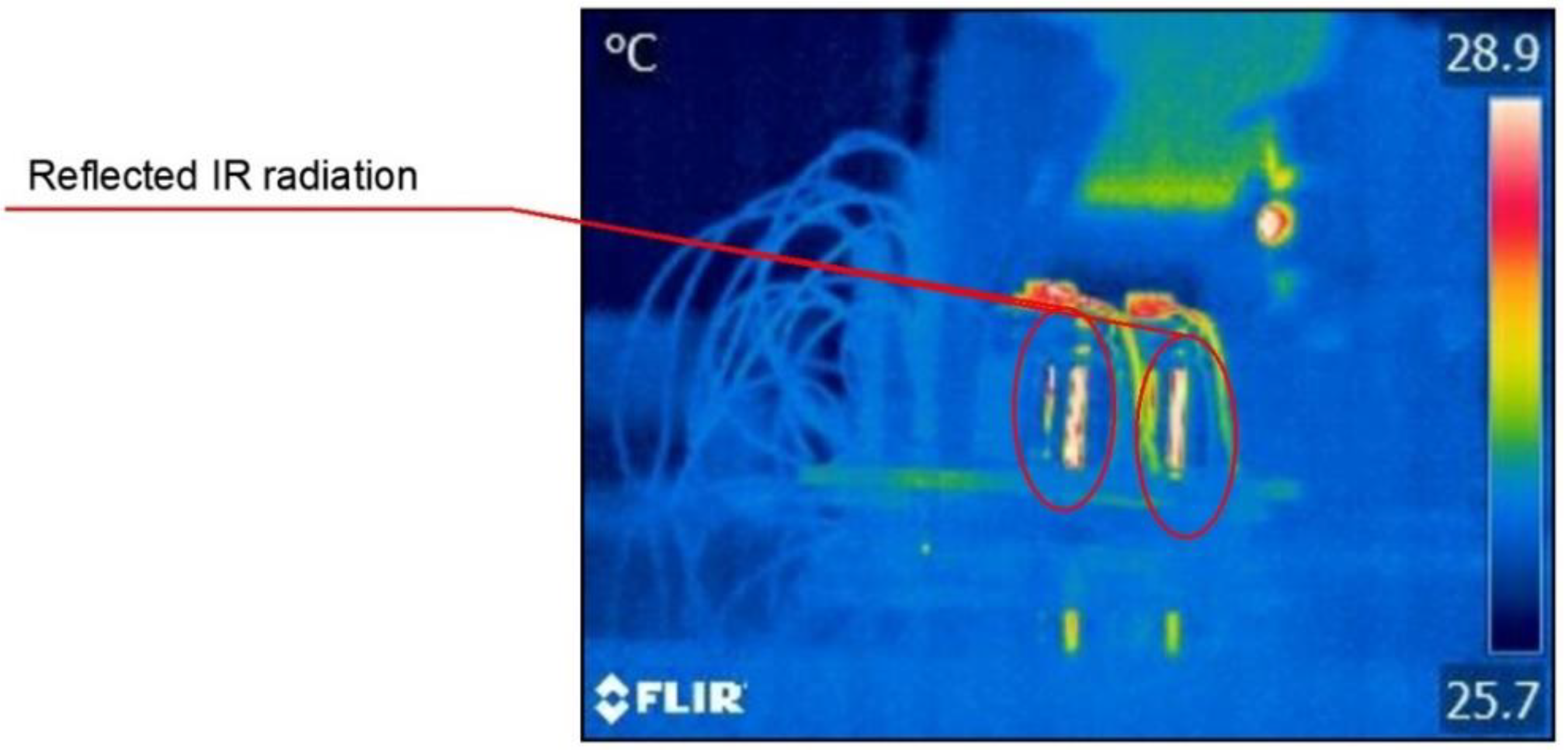
2.1.3. Reflected Temperature

Reflected temperature ϑ_refl is also called reflected radiation [32] in the literature. It is the radiation emitted by an object that is in the vicinity of the object under observation. The reflected radiation reaches the lens of the thermographic camera together with the radiation emitted by the object under observation. There is no mathematical model that would accurately describe the value of ϑ_refl in every case. For this reason, to minimize the influence of ϑ_refl on the value of ϑ_obj, the value of ϑ_refl should always be measured. The measured value of ϑ_refl should be entered in the software of the thermographic camera before checking the degree of heating of individual capacitor cells. The relationship between ϑ_obj and ϑ_refl can be described by Equation (3).

For a better explanation, the discussed phenomenon is presented in Figure 4.

An example of the recorded reflected radiation is shown in Figure 5, where capacitors used for compensating reactive power can be seen. Reflected radiation was registered on both capacitor cases, which were made of aluminum.

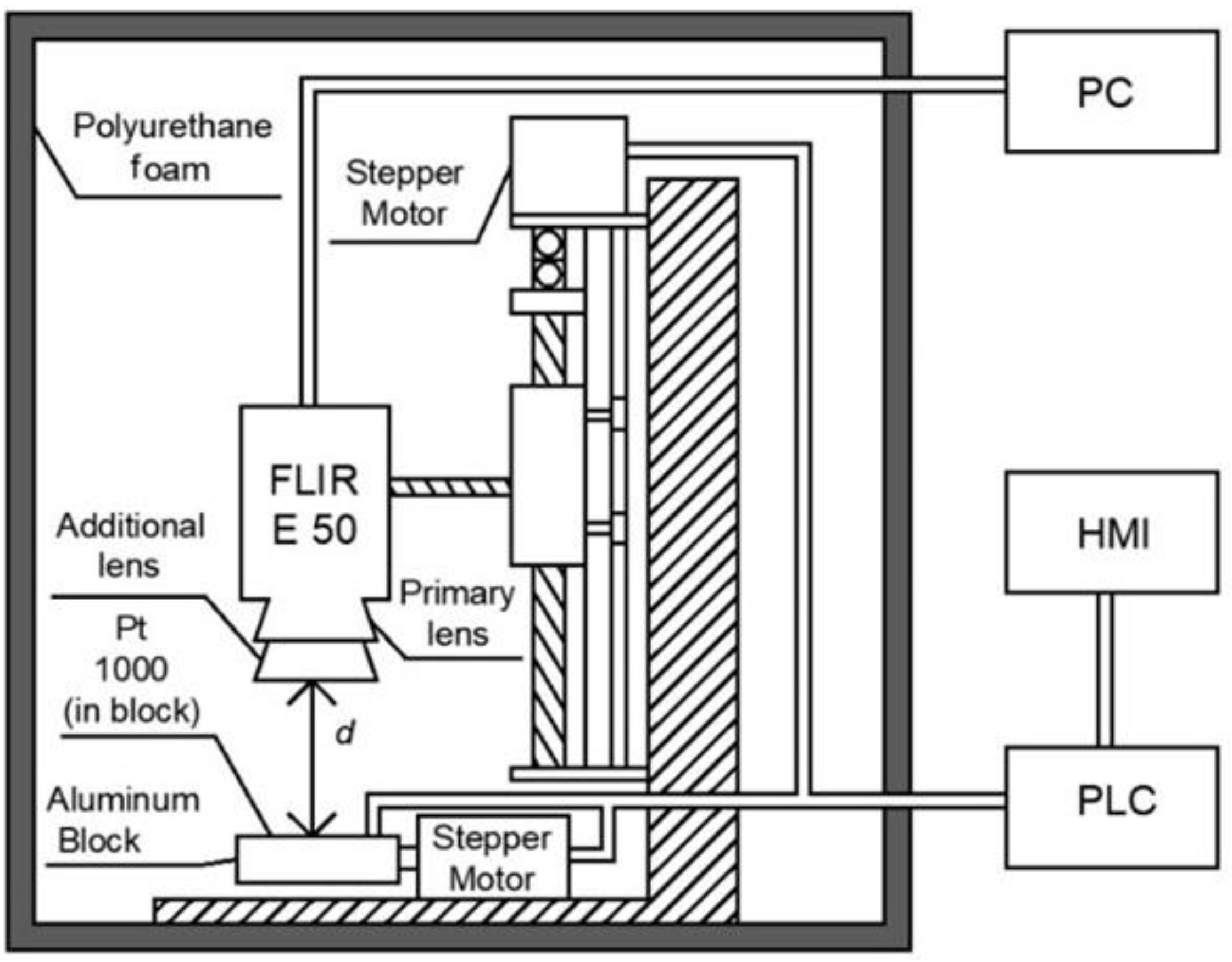
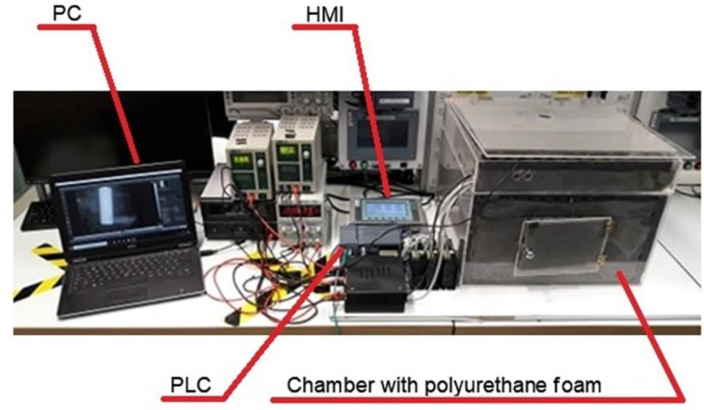
2.2. The Measurement System

The first part of the experiments described in this article was carried out using a specially constructed stand. The stand consisted of three parts: a chamber with the measuring instruments, a control part, and a laptop with Flir Tools + software. The most important device in the stand was the Flir E50 thermographic camera (Flir, Wilsonville, OR, USA) [33]. In order to obtain appropriate spatial resolution, the camera was equipped with an additional Close-up 2× lens (Flir, Wilsonville, OR, USA). This made it possible to obtain an IFOV (Instantaneous Field of View) of 67 µm [34]. The camera with an additional lens was mounted on a linear module. In turn, the linear module was attached to a metal angle. The linear module was controlled by a stepper motor [35]. Consequently, it was possible to change d with a precision of 0.1 mm. The distance d was controlled by means of an appropriately mounted potentiometric offset sensor MMR30, with a nominal resistance value of 10 kΩ [36]. This sensor made it possible to measure the distance d in the range of 0–30 mm, with a precision of 0.1 mm. At a distance of about 30 mm from the lens, an aluminum block sized 16 mm × 16 mm × 45 mm was placed. The surface of the block, monitored with a thermographic camera, was painted with Velvet Coating 811-21. The block temperature was monitored with a Pt 1000 sensor [37]. The monitored block was connected to a stepper motor. Consequently, it was possible to change α with a precision of 0.9°. In order to run the indivudual parts of the experiment, the block was replaced with a heating plate of a known temperature. The entire set was placed in a chamber made of plexiglass with the external dimensions of 45 cm × 45 cm × 33 cm. In order to minimize the influence of reflections and ensure proper optical isolation, the interior of the chamber was lined with black polyurethane foam. Due to the porous structure of the foam and its color the value of factor ε equaled 0.95 [38] inside the chamber. Additionally, the metal components inside the chamber were painted black. Using the Siemens S7-1200 1214C DC/DC/DC PLC controller (Siemens AG, Munich, Germany) [39], all actuators and readings were made from the sensors. This controller supported the HMI touch panel (Siemens AG, Munich, Germany) [40], by means of which it was possible to set the required settings and read them.

The camera was connected to the laptop via a USB interface. Using the Flir Tools + software during the experiment, the settings of the thermographic camera were changed. It was also possible to record thermograms. The diagram of the described stand is presented in Figure 6.

A photo of the presented stand is shown in Figure 7.

The second part of the experiment was carried out on a stand consisting of a Flir E50 thermographic camera (without an additional lens) and the tested capacitors for reactive power compensation. The capacitors were star-connected to increase their temperature to the operating temperature, higher than the ambient temperature. The distance between the capacitors and the lens was measured with a precision of 1 cm. In the last part of the work, the capacitors were changed to a cylinder made of aluminum with an adjustable diameter. A piece of metal (aluminum), which was industrial waste, measuring 90 cm × 4 cm was used. Using that method, attempts were made to recreate the conditions prevailing during the thermographic temperature measurement of the operated capacitor bank. A diagram of the measuring system is shown in Figure 8.

A photo of the system, which has been described and showed in Figure 8, is presented in Figure 9.

3. Results

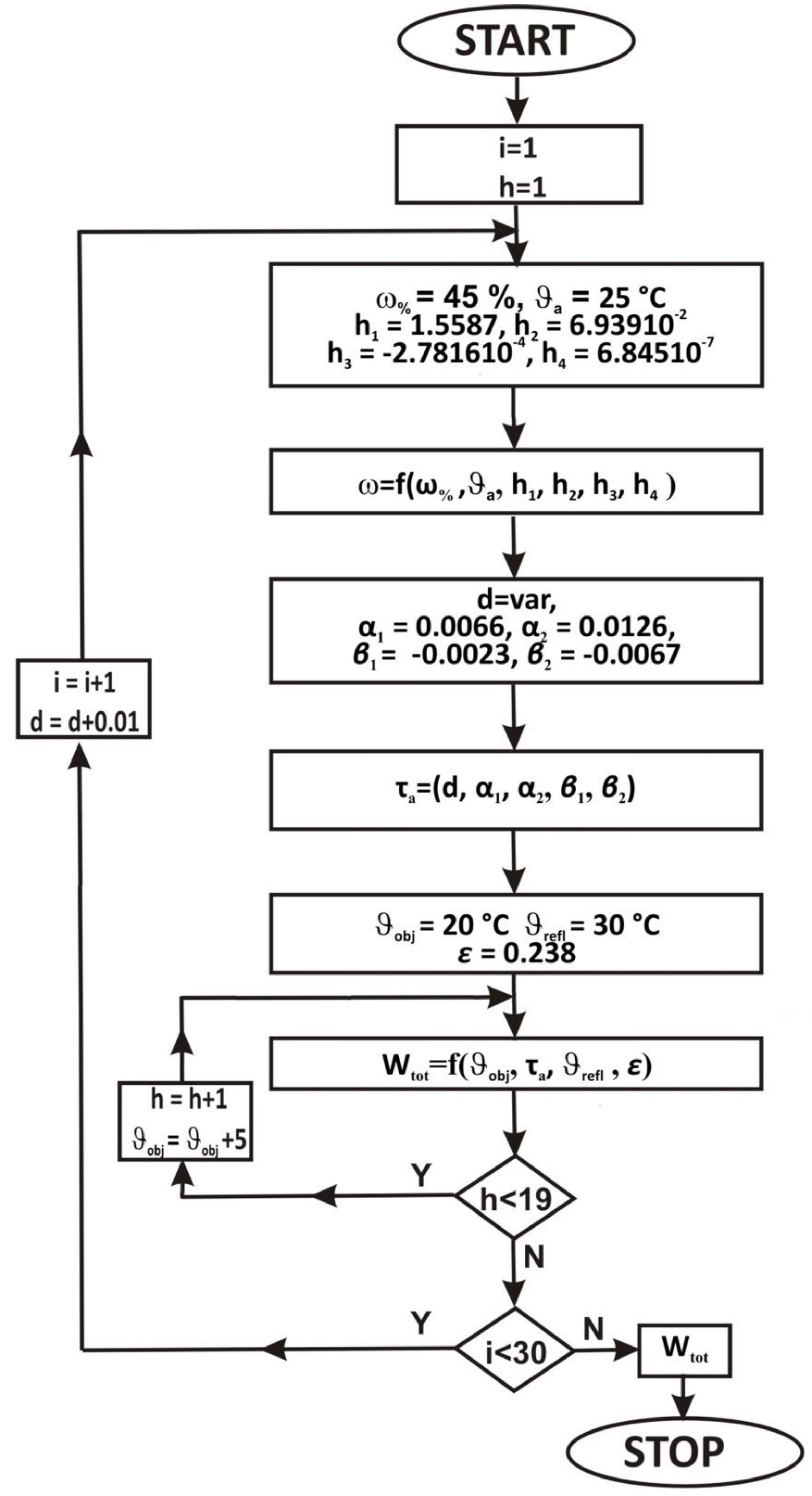
3.1. Results of Simulation Tests

As a result of the simulation work carried out, it was checked how the result of the ϑ_t value would change due to the change in d caused by placing the measurement point on various parts of the case. Based on the analysis of the available technical documentation, it was assumed that the diameter of the capacitor case intended for reactive power compensation would not exceed 3000 mm. This means that the difference between the largest and smallest d values will not be bigger than 1500 mm [41]. The simulation was performed for standard conditions (ϑ_a = 25 °C). The half of the range of values recorded in the laboratory (45%) was adopted as the value of ω_%. The given criteria were followed by selecting the ϑ_refl value of 30 °C. The ε was chosen for aluminum (ε = 0.238). It was assumed that the range d would be changed from 0.85 m to 0.15 m. It was an arbitrarily adopted distance of 1 m changed by the range resulting from the largest assumed capacitor diameter. During the simulation, the value of d was changed with the step of i = 0.01.

In the first part of the simulation, the W_tot value was determined for the ϑ_obj value in the range from −20 °C to 70 °C, changed in steps h = 5 °C. The lower value of the assumed range, ϑ_obj, is the assumed ambient temperature. The upper limit of the range is the highest possible temperature of the capacitor case that can be found in the catalogs. During the simulation, the W_tot values were determined according to the algorithm shown in Figure 10 for all variable values. The values of the coefficients used were taken from [29].

After determining the value of W_tot, the values of ϑ_cam were determined for each value of d and ϑ_obj. The graph obtained as a result of the simulation, showing the changes of ϑ_cam as a function of d, for different values of ϑ_obj, is shown in Figure 11.

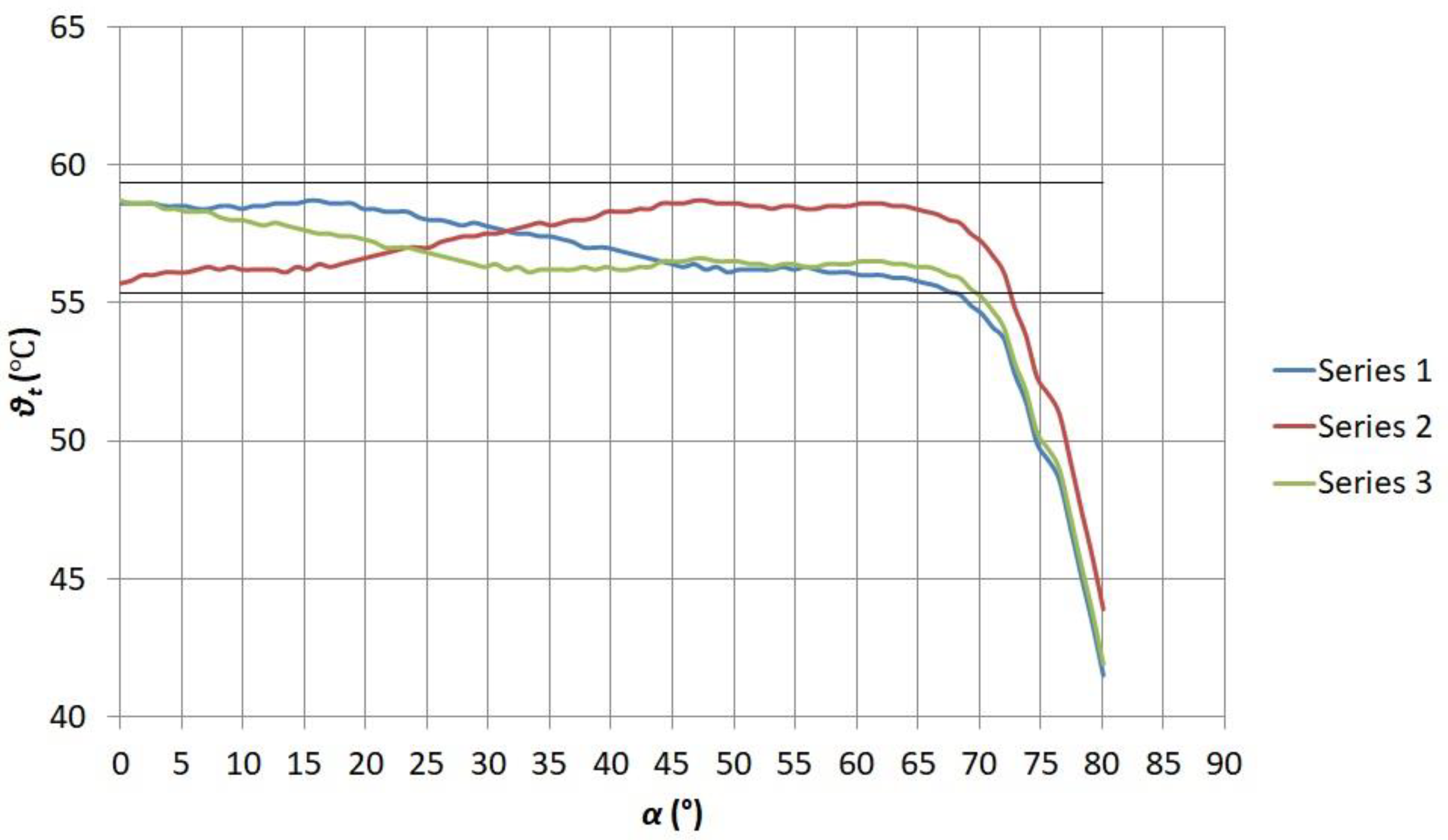
3.2. Influence of Angle of View on the Value of Thermographic Temperature Measurement of Small Diameter Cases

In order to check the influence of α on the value of ϑ_t, it was decided to repeat the experiment carried out by one of the authors of this article and described in [42]. This was performed to obtain the data that would allow us to estimate the influence of the α value on the ϑ_cam value in the case of thermographic temperature measurements on the cases capacitors intended for reactive power compensation. An aluminum block with a known temperature of 57.35 °C was observed. In order to minimize the impact of the changing conditions during the measurement, measurements were made by automatic changing of α and simultaneous film recording with a thermographic camera. The results were obtained by analyzing individual frames of the recorded film. The results were made for three series of measurements. The achieved results are shown in Figure 12. In the figure, the black lines indicate the value of the known temperature of the block under observation increased or decreased by the measurement error of the thermographic camera [34].

The aluminum block was then replaced with a temperature-controlled heating plate. During the measurements, the plate was placed parallel to the lens of the thermographic camera. The capacitors covered with Velvet Coating 811-21 paint were put on the plate. The paint was applied to a thin plastic layer that was on the capacitor. After the temperature of the capacitor was established, a thermogram was made. Examples of thermograms are presented in Figure 13.

The ϑ_t values recorded in the thermogram were exported to Excel. The recorded values of ϑ_t as a function of the position on the case x are shown in Figure 14 and Figure 15. The initial value (x = 0 mm) was the point of the capacitor case that was closest to the thermographic camera lens (in the middle of the capacitor case).

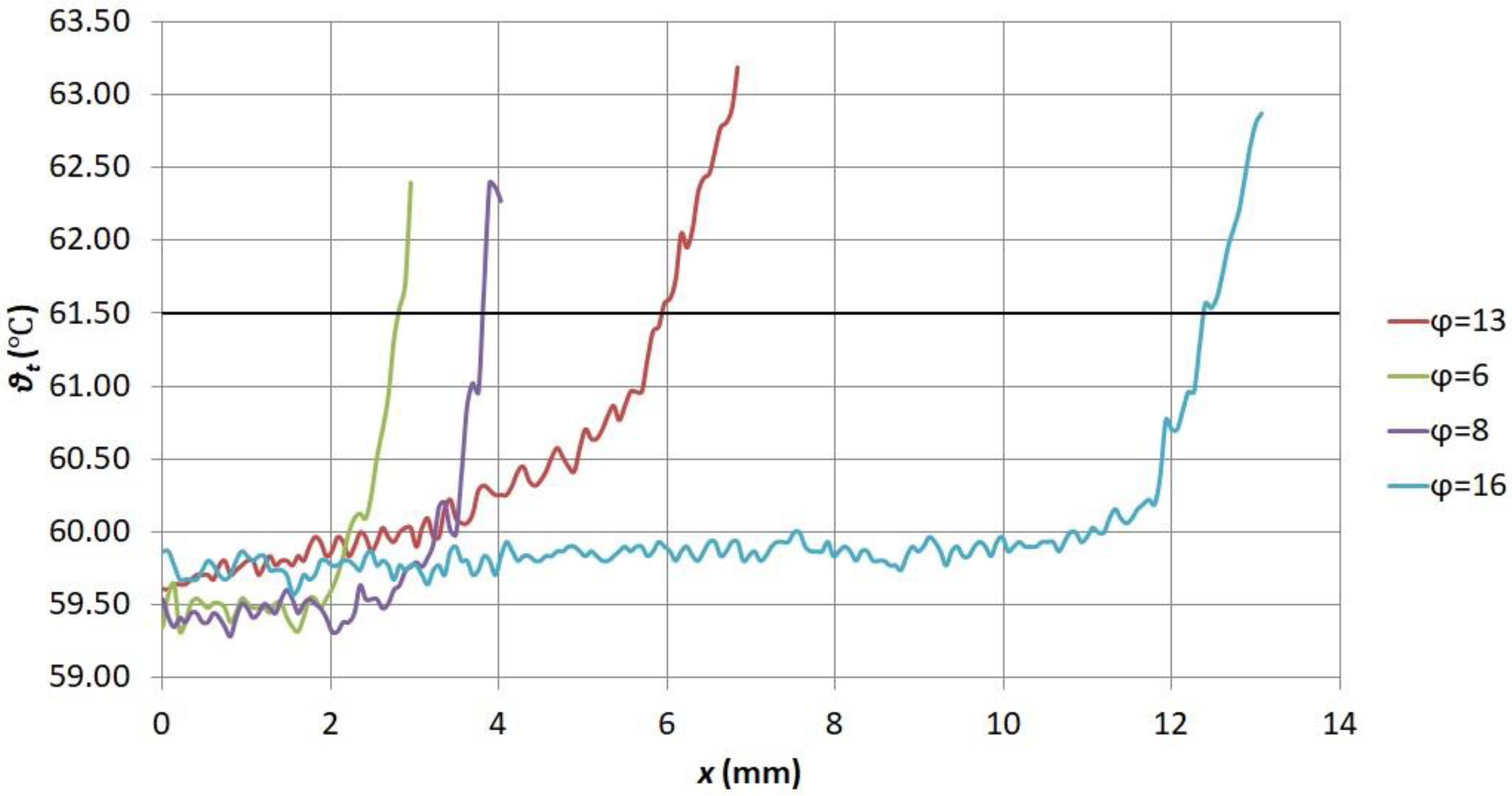
3.3. Influence of Angle of View on the Value of Thermographic Temperature Measurement of a Typical Case

At the beginning, it was decided to experimentally check the simulation results presented in Figure 6. For that purpose, the KJF-0.83/400 capacitors were star-connected and loaded with the rated current (Figure 9). The distance d was changed in the range from 0.85 m to 1.15 m. With a step equal to 0.01 m and for each distance, a thermogram was made. The results of thermographic temperature measurements are shown in Figure 16.

Then, the edge length of the field of view of a single detector of the thermographic camera I was checked, while the distance d was 1 m. The formula (10) was used. The determined value of I was 1.82 mm:

$$I=2\cdot d\cdot tg(\frac{\mathrm{IFOV}}{2})$$

(10)

where IFOV is the value of the angle between the adjacent walls of the pyramid, read from the technical documentation of the thermographic camera, the apex of which is in the IR detector of the camera and the base of the object under observation. For Flir E50, IFOV equals 1.82 mrad. Knowing the value of I, the temperature distribution (function ϑ_t = f(x)) was checked on the metal case of the KJF-0.83/400 capacitors. An example thermogram is presented in Figure 17.

The capacitors were star-connected and loaded with the rated current. The distance d was 1 m. The remaining parameters corresponded to the conditions prevailing during the measurement (ε = 0.24, ϑ_refl = 26 °C, ϑ_l = 26 °C, τ_l = 1, ω_% = 45%). The value of ϑ_refl was measured by placing a bent aluminum foil on the case of the observed capacitor and changing the settings of ε = 1, d = 0. The value of ϑ_refl was the one indicated by the thermographic camera. The obtained functions ϑ_t = f(x) for three capacitors are shown in Figure 18. The point located in the middle of the capacitor case was assumed as x = 0.

In order to make the work more universal, it was decided to check whether a similar temperature distribution (the function ϑ_t = f(x)) would also be recorded on cylindrical aluminum surfaces with different cross-sections. For this purpose, an aluminum strip measuring 4 cm by 90 cm was rolled up. It was decided to check the temperature distribution on a cylinder with a diameter of 100 mm and 130 mm. The center of the observed surface was taken as x = 0 again. The thermographic camera settings were as follows: ε = 0.24, ϑ_refl = 26 °C, ϑ_l = 26 °C, τ_l = 1, ω_% = 45%, d = 1 m. The obtained results are shown in Figure 19.

4. Conclusions

Thermography is a method that makes it possible to check the degree of heating of the cells in a capacitor bank. Regular performance of thermograms enables safe detection of the increase in surface heating of the observed capacitor. It is worth remembering to compare thermograms made with the same settings of the thermographic camera.

The temperature values measured on different parts of the capacitor case may differ from each other. This phenomenon may be due to the local properties of the material fragment. Regarding the observed cylindrical cases, the influence of two phenomena was considered: the different distances of the thermographic camera lens, the object under observation, and the angular emissivity.

When analyzing the graphs in Figure 14, Figure 15 and Figure 16, it can be noticed that in the case of small capacitors (φ ≤ 30 mm), the error of the thermographic temperature measurement caused by an incorrect selection of a point on the capacitor case will not exceed 3 °C. In the case of large capacitors (φ ≥ 30 mm), this value will not exceed 1 °C (Figure 18 and Figure 19). It needs to be emphasized that in the case of thermographic observations of small capacitors, an additional macro lens was used. One should also remember the error of the thermal imaging camera, amounting to ±2 °C or ±2% of reading, for ambient temperature between 10 °C and 35 °C.

In the conducted works, the Flir E50 thermographic camera was used. In the camera software, you can compensate the influence of the distance between the lens and the object under observation with a resolution of one meter. In the case of the observed phenomenon, changes in this distance are smaller. At the stage of simulation tests, it was already shown that a change in the distance of the thermographic camera lens from the object under observation, amounting to less than 15 cm, would not cause a significant change in the temperature indicated by the thermographic camera (Figure 11).

Angular emissivity has a bigger influence on the change in the result of thermographic temperature measurement. As a result of the conducted experimental works, the dependence of the result of thermographic measurement of capacitor surface temperature on the angle of view was demonstrated. In addition, it was shown that the shape of the both characteristic—the result of the thermographic temperature measurement and the angle of view—would be different for a metal surface of the capacitor and different for the surface of the capacitor covered with plastic. The change in the thermographic temperature measurement result above the error value of the thermographic camera occurs for large viewing angles (approx. 67°).

It can be concluded that the change in the thermographic temperature measurement result due to changes in the position of the observed point on the case is mainly caused by angular emissivity. Only extreme positions of the observed point on the capacitor case should be avoided. The effect of reflected radiation is random and difficult to determine.

References

1. Kuwałek, P. Estimation of Parameters Associated with Individual Sources of Voltage Fluctuations. IEEE Trans. Power Deliv. 2021, 36, 351–361. [Google Scholar] [CrossRef]
2. Ermolaev, D.; Plekhov, A.; Titov, D.; Vagapov, Y. Vibration damping in a motor drive shaft system operating under active power flow oscillation. In Proceedings of the 2018 IEEE Conference of Russian Young Researchers in Electrical and Electronic Engineering (EIConRus), St. Petersburg, Russia, 29 January–1 February 2018; pp. 1723–1727. [Google Scholar] [CrossRef]
3. Anttila, A.; Aarniovuori, L.; Niemelä, M.; Zaheer, M.; Lindh, P.; Pyrhönen, J. Active Power Analysis of PWM-driven Induction Motor in Frequency Domain. In Proceedings of the 2021 XVIII International Scientific Technical Conference Alternating Current Electric Drives (ACED), Ekaterinburg, Russia, 28 February 2021; pp. 1–6. [Google Scholar] [CrossRef]
4. Chen, Y.; Zhao, X.; Yang, Y.; Shi, Y. Online Diagnosis of Inter-turn Short Circuit for Dual-Redundancy Permanent Magnet Synchronous Motor Based on Reactive Power Difference. Energies 2019, 12, 510. [Google Scholar] [CrossRef] [Green Version]
5. Graña-López, M.A.; García-Diez, A.; Filgueira-Vizoso, A.; Chouza-Gestoso, J.; Masdías-Bonome, A. Study of the Sustainability of Electrical Power Systems: Analysis of the Causes that Generate Reactive Power. Sustainability 2019, 11, 7202. [Google Scholar] [CrossRef] [Green Version]
6. Yani, A.; Junaidi, J.; Irwanto, M.; Haziah, A.H. Optimum reactive power to improve power factor in industry using genetic algortihm. Indones. J. Electr. Eng. Comput. Sci. 2019, 14, 751–757. [Google Scholar] [CrossRef]
7. Van Huyen, D.; Thanh Hien, P.; Cuong, N.D. Design of Dynamic—Static VAr compensation based on microcontroller for improving power factor. In Proceedings of the 2017 International Conference on System Science and Engineering (ICSSE), Ho Chi Minh City, Vietnam, 21–23 July 2017; pp. 186–190. [Google Scholar] [CrossRef]
8. Ernst, S.; Kotulski, L.; Lerch, T.; Rad, M.; Sędziwy, A.; Wojnicki, I. Application of reactive power compensation algorithm for large-scale street lighting. J. Comput. Sci. 2021, 51, 101338–101346. [Google Scholar] [CrossRef]
9. Kabir, Y.; Mohsin, Y.M.; Khan, M.M. Automated power factor correction and energy monitoring system. In Proceedings of the 2017 Second International Conference on Electrical, Computer and Communication Technologies (ICECCT), Coimbatore, India, 22–24 February 2017; pp. 1–5. [Google Scholar] [CrossRef]
10. Nitulescu, M.; Al-Atwan, N.S.S. A Solution for Controlling the Parameters of Electricity Consumption in an Intelligent Home. In Proceedings of the 22nd International Carpathian Control Conference (ICCC), Ostrava, Czech Republic, 31 May–1 June 2021; pp. 1–6. [Google Scholar] [CrossRef]
11. El Ghossein, N.; Sari, V.; Venet, P.; Genies, S.; Azaïs, P. Post-Mortem Analysis of Lithium-Ion Capacitors after Accelerated Aging Tests. J. Energy Storage 2021, 33, 102039–102049. [Google Scholar] [CrossRef]
12. Teli, L.V.; Jadhav, H.T. A Review on Protection of Capacitor in Power Quality Industry. In Proceedings of the International Conference on Current Trends towards Converging Technologies (ICCTCT), Coimbatore, India, 1–3 March 2018; pp. 1–5. [Google Scholar] [CrossRef]
13. Bolufawi, O.; Shellikeri, A.; Zheng, J.P. Lithium-Ion Capacitor Safety Testing for Commercial Application. Batteries 2019, 5, 74. [Google Scholar] [CrossRef] [Green Version]
14. Available online: https://www.udt.gov.pl/laboratorium-badawcze-ab-001/metoda-badan/badania-materialowe-nieniszczace (accessed on 7 July 2021).
15. Zaccara, Z.; Edelman, J.B.; Cardone, G. A general procedure for infrared thermography heat transfer measurements in hypersonic wind tunnels. Int. J. Heat Mass Transf. 2020, 163, 120419–120435. [Google Scholar] [CrossRef]
16. Altenburg, J.S.; Straße, A.; Gumenyuk, A.; Meierhofer, C. In-situ monitoring of a laser metal deposition (LMD) process: Comparison of MWIR, SWIR and high-speed NIR thermography. Quant. InfraRed Thermogr. J. 2020, 1–18. [Google Scholar] [CrossRef]
17. Yoon, S.T.; Park, J.C. An experimental study on the evaluation of temperature uniformity on the surface of a blackbody using infrared cameras. Quant. InfraRed Thermogr. J. 2021, 1–15. [Google Scholar] [CrossRef]
18. Schuss, C.; Remes, K.; Leppänen, K.; Saarela, J.; Fabritius, T.; Eichberger, B.; Rahkonen, T. Detecting Defects in Photovoltaic Cells and Panels with the Help of Time-Resolved Thermography under Outdoor Environmental Conditions. In Proceedings of the 2020 IEEE International Instrumentation and Measurement Technology Conference (I2MTC), Dubrovnik, Croatia, 25–28 May 2020; pp. 1–6. [Google Scholar] [CrossRef]
19. Chakraborty, B.; Billol, K.S. Process-integrated steel ladle monitoring, based on infrared imaging—A robust approach to avoid ladle breakout. Quant. InfraRed Thermogr. J. 2020, 169–191. [Google Scholar] [CrossRef]
20. Tomoyuki, T. Coaxiality Evaluation of Coaxial Imaging System with Concentric Silicon-Glass Hybrid Lens for Thermal and Color Imaging. Sensors 2020, 20, 5753. [Google Scholar] [CrossRef]
21. Singh, J.; Arora, A.S. Effectiveness of active dynamic and passive thermography in the detection of maxillary sinusitis. Quant. InfraRed Thermogr. J. 2020, 18, 1–13. [Google Scholar] [CrossRef]
22. Litwa, M. Influence of angle of View on Temperature Measurement Using Thermovision Camera. IEEE Sens. J. 2010, 10, 1552–1554. [Google Scholar] [CrossRef]
23. User’s Manual Flir Tools/Tools+. Available online: http://91.143.108.245/Downloads/Flir/Dokumentation/t810209-en-us_a4.pdf/ (accessed on 28 May 2021).
24. Dziarski, K.; Hulewicz, A.; Dombek, G. Lack of Thermogram Sharpness as Component of Thermographic Temperature Measurement Uncertainty Budget. Sensors 2021, 21, 4013. [Google Scholar] [CrossRef] [PubMed]
25. Zhang, Y.; Liu, L.; Gong, W.; Yu, H.; Wang, W.; Zhao, C.; Wang, P.; Ueda, T. Autofocus System and Evaluation Methodologies: A Literature Review. Sens. Mater. 2018, 30, 1165. [Google Scholar] [CrossRef]
26. Sivakumar, K.; Prasad, A.R.; Jagadesh, T.; Kumar, S.D.; Ponshanmugakumar, A.; Thamilarasan, K. Experimental investigation on emissivity of 75Ni-25Cr alloy coated Aluminium surface for the purpose of solar applications. Mater. Today: Proc. 2021, 37, 1320–1323. [Google Scholar]
27. He, L.; Zhao, Y.; Xing, L.; Liu, P.; Zhang, Y.; Wang, Z. Low Infrared Emissivity Coating Based on Graphene Surface-Modified Flaky Aluminum. Materials 2018, 11, 1502. [Google Scholar] [CrossRef] [PubMed] [Green Version]
28. Więcek, B.; Pacholski, K.; Olbrycht, R.; Strakowski, R.; Kałuża, M.; Borecki, M.; Wittchen, W. Termografia I Spektrometria w Podczerwieni; WNT: Warszawa, Poland, 2017; pp. 42–44. ISBN 9788301191870. [Google Scholar]
29. Minkina, W.; Klecha, D. Modeling of Athmospheric Transmission Coefficient in Infrared for Thermography Measurements. In Proceedings of the Sensor 2015 and IRS2 2015 AMA Conferences, Nürnberg, Germany, 19–21 May 2015. [Google Scholar] [CrossRef]
30. Tran, Q.H.; Han, D.; Kang, C.; Haldar, A.; Huh, J. Effects of Ambient Temperature and Relative Humidity on Subsurface Defect Detection in Concrete Structures by Active Thermal Imaging. Sensors 2017, 17, 1718. [Google Scholar] [CrossRef] [PubMed]
31. Więcek, B.; De Mey, G. Termowizja w Podczerwieni Podstawy i Zastosowania; PAK: Gliwice, Poland, 2011; pp. 42–44. ISBN 9788392631972. [Google Scholar]
32. Hulewicz, A.; Dziarski, K.; Dombek, G. The Solution for the Thermographic Measurement of the Temperature of a Small Object. Sensors 2021, 21, 5000. [Google Scholar] [CrossRef]
33. Flir E-Series. Available online: https://www.globaltestsupply.com/pdfs/cache/www.globaltestsupply.com/flir_systems/thermal_imager/e50/datasheet/flir_systems_e50_thermal_imager_datasheet.pdf (accessed on 15 June 2021).
34. Close-Up 2× Lens. Available online: https://www.flircameras.com/t197214-close-up-2x-lens.htm (accessed on 15 June 2021).
35. Linear Motion Rail. Available online: https://www.ebay.com/itm/144058129406?nma=true&si=zDq%252FAdKaAs9Fgk6cIp8AHgHHQbI%253D&orig_cvip=true&nordt=true&rt=nc&_trksid=p2047675.l2557 (accessed on 15 June 2021).
36. Data Sheet for Linear Sensors. Available online: http://www.czujniki.org/download/ds_mm_dt.pdf (accessed on 3 April 2021).
37. Data Sheet for Pt 1000. Available online: https://www.tme.eu/Document/67cf717905f835bc5efcdcd56ca3a8e2/Pt1000-550_EN.pdf (accessed on 15 July 2021).
38. Krawiec, P.; Rózański, L.; Czarnecka-Komorowska, D.; Warguła, Ł. Evaluation of the Thermal Stability and Surface Characteristics of Thermoplastic Polyurethane V-Belt. Materials 2020, 7, 1502. [Google Scholar] [CrossRef] [PubMed] [Green Version]
39. PLC Controller. Available online: https://docs.rs-online.com/4ed5/0900766b81397276.pdf (accessed on 15 June 2021).
40. HMI Panel. Available online: https://static.rapidonline.com/pdf/543842_v1.pdf (accessed on 15 June 2021).
41. Capacitor. Available online: https://legrand.pl/system/files/download/kompensacja_mocy_biernej_legrand_-_katalog.pdf (accessed on 15 June 2021).
42. Dziarski, K. Selection of the Observation Angle in Thermography Temperature Measurements with the Use of a Macro Lens. In Proceedings of the International Conference on Measurement, Smolenice, Slovakia, 17–19 May 2021; pp. 101–104. [Google Scholar] [CrossRef]
Figure 1. Thermograms presenting the Pt 1000 temperature sensor in a cylindrical case with a diameter of 3 mm. Thermograms were taken at the same distance between the sensor and the lens of the thermal imaging camera. The sensor temperature was 49.6 °C. Temperature measured in Sp: (a) 49.6 °C; (b) 48.5 °C; (c) 47.7 °C.
Energies 14 05736 g001
Figure 2. Thermograms presenting the electrolytic capacitor in a cylindrical case with a diameter of 4 mm. Thermograms were taken at the same distance between the sensor and the lens of the thermographic camera. The temperature of the heating mat on which the capacitor was placed was 60 °C. Temperature measured in Sp: (a) 59.5 °C; (b) 59.3 °C; (c) 58.8 °C.
Energies 14 05736 g002
Figure 3. Distances between the thermographic camera lens and points on the capacitor case.
Energies 14 05736 g003
Figure 4. Selected components of radiation reaching the lens of a thermographic camera: (1) reflected radiation; (2) radiation emitted by the capacitor case.
Energies 14 05736 g004
Figure 5. Reflected radiation, registered on two metal cases of capacitors KJF 0.83/400. The reflected radiation is marked with circles.
Energies 14 05736 g005
Figure 6. Diagram of the stand used in the first part of the experiments.
Energies 14 05736 g006
Figure 7. Photograph of the constructed measuring stand.
Energies 14 05736 g007
Figure 8. Diagram of the measuring system used in the second part of the experiments. d is the distance between the thermographic camera lens and the object under observation and C1–C3 are the capacitors used in the experiments.
Energies 14 05736 g008
Figure 9. Photograph of the measurement system used in the second part of the experiments.
Energies 14 05736 g009
Figure 10. The search algorithm of maximum Wtot value, as well as the search algorithm of the minimum Wtot value.
Energies 14 05736 g010
Figure 11. Change in the result of the thermographic temperature measurement ϑcam depending on the change in d, for different values of ϑobj.
Energies 14 05736 g011
Figure 12. Change in the result of the thermographic temperature measurement ϑt depending on the change in α. The black lines indicate the value of the known temperature of the block under observation, increased or decreased by the measurement error of the thermographic camera.
Energies 14 05736 g012
Figure 13. Thermograms for capacitors with different diameters φ (a) φ = 16, ϑt in Sp1 = 59.6 °C (b) φ = 13, in Sp1 = 60.6 °C (c) φ = 6, in Sp1 = 59.3 °C. ϑt is the result of thermal imaging temperature measurement.
Energies 14 05736 g013
Figure 14. Diagram of ϑt = f(x) for capacitor cases of different diameters. The temperature of the heating plate was 59.5 °C. The black line indicates the temperature of the heating plate increased by the measurement error of the thermographic camera (61.5 °C).
Energies 14 05736 g014
Figure 15. Diagram of ϑt = f(x) for capacitor cases of different diameters. The temperature of the heating plate was 52.3 °C. The black line indicates the temperature of the heating plate increased by the measurement error of the thermographic camera (54.3 °C).
Energies 14 05736 g015
Figure 16. Relationship ϑt = f(d) obtained experimentally.
Energies 14 05736 g016
Figure 17. Example thermogram for KJF-0.83/400 capacitors.
Energies 14 05736 g017
Figure 18. Diagram of ϑt = f(x) for the cases of KJF-0.83/400 capacitors loaded with the rated current.
Energies 14 05736 g018
Figure 19. Diagram of ϑt = f(x) for aluminum cylinders with a diameter of ϕ = 100 mm and ϕ = 130 mm.
Energies 14 05736 g019
Publisher’s Note: MDPI stays neutral with regard to jurisdictional claims in published maps and institutional affiliations.