Article

Verification and Validation of COMSOL Magnetohydrodynamic Models for Liquid Metal Breeding Blankets Technologies

1
ESSENTIAL Group, Politecnico di Torino—Corso Duca degli Abruzzi, 24, 10129 Torino, Italy
2
ENEA FSN-PROIN, C.R. Brasimone—Località Brasimone, 40043 Camugnano, Italy
3
PSFC, MIT, Massachusetts Institute of Technology, Cambridge, MA 02139, USA
*
Author to whom correspondence should be addressed.
Energies 2021, 14(17), 5413; https://doi.org/10.3390/en14175413
Submission received: 21 July 2021 / Revised: 18 August 2021 / Accepted: 26 August 2021 / Published: 31 August 2021
(This article belongs to the Special Issue Thermal-Hydraulics in Nuclear Fusion Technology: R&D and Applications)

Abstract

:
Liquid metal breeding blankets are extensively studied in nuclear fusion. In the main proposed systems, the Water Cooled Lithium Lead (WCLL) and the Dual Coolant Lithium Lead (DCLL), the liquid metal flows under an intense transverse magnetic field, for which a magnetohydrodynamic (MHD) effect is produced. The result is the alteration of all the flow features and the increase in the pressure drops. Although the latter issue can be evaluated with system models, 3D MHD codes are of extreme importance both in the design phase and for safety analyses. To test the reliability of COMSOL Multiphysics for the development of MHD models, a method for verification and validation of magnetohydrodynamic codes is followed. The benchmark problems solved regard steady state, fully developed flows in rectangular ducts, non-isothermal flows, flow in a spatially varying transverse magnetic field and two different unsteady turbulent problems, quasi-two-dimensional MHD turbulent flow and 3D turbulent MHD flow entering a magnetic obstacle. The computed results show good agreement with the reference solutions for all the addressed problems, suggesting that COMSOL can be used as software to study liquid metal MHD problems under the flow regimes typical of fusion power reactors.

1. Introduction

In the nuclear fusion framework, the breeding blanket is a key system devoted to power extraction, shielding and tritium production. Among the different designs of the blanket, in the Water-Cooled Lithium-Lead (WCLL) breeding blanket of DEMO [1] and in the WCLL test blanket module of ITER, the liquid, electrically conducting LiPb is adopted as working fluid to address the above-mentioned functions. The intense magnetic field used in fusion reactors to confine the burning plasma has a strong influence on the flow behavior, producing a magnetohydrodynamic (MHD) effect. In addition, serious temperature gradients are present in the breeding blanket, giving rise to buoyancy forces. The presence of the external magnetic field produces an additional MHD pressure drop, and although rougher MHD studies can predict the ∆p [2], other phenomena, such as turbulence and buoyancy-driven convection, have a drastic impact on blanket performance and require a deeper analysis. In addition, tritium transport mechanisms [3,4,5] are influenced by the magnetic field; therefore, a detailed solution of magnetohydrodynamics is necessary, and it is obtainable with 3D multiphysics models for the breeding blanket. Smolentsev et al. [6] proposed activity for verification and validation of MHD codes for fusion applications, consisting of a series of benchmark problems whose results are known from experimental data or trusted analytical and numerical solutions. In particular, the five problems cover a wide range of magnetohydrodynamic flows which are of interest for fusion applications:
  • 2D fully developed laminar steady flow;
  • 3D laminar, steady developing flow in a nonuniform magnetic field;
  • Buoyancy-driven flow in a square cavity;
  • Quasi-two-dimensional (Q2D) turbulent flow;
  • 3D turbulent flow.
In this work, a verification and validation procedure of the developed 3D codes is performed, taking as reference [6]. Verification and validation activities of MHD codes were conducted by different authors for 1D codes [7], 3D codes under the COMSOL environment [8] and other codes [9,10,11,12]. Here, in order to further extend the analysis performed by [8], two benchmark cases involving unsteady flows are solved. The Q2D turbulence case proposed by Burr [13] was solved by adopting a modified version of the kε model, derived by [14], while the fully 3D turbulent problem was tackled using the Large Eddy Simulation (LES) Residual Based Variational Multiscale (RBVM) method [15,16,17]. For the magnetoconvection case, the problems selected are the ones proposed by Di Piazza and Buhler [18], which are of particular interest for liquid metal breeding blanket technologies. In effect, in the first problem, the non-isothermal condition is due to differentially heated boundaries, while in the second case, temperature gradients are produced by internal heat generation. Both conditions are typical in breeding blanket systems, where strong temperature gradients and intense volumetric heat generation are present.

2. Governing Equations

The flow of liquid metal in breeding blanket conditions is characterized by a small magnetic Reynolds number R m = μ σ L U (−). Here, μ (Pa s) and σ (S m−1) are, respectively, the dynamic viscosity and the electrical conductivity of the fluid, L (m) and U (m s−1) are the characteristic length and velocity of the flow. The magnetic Reynolds number represents the ratio between induction and diffusion of the magnetic field, so, in the low- R m approximation, the magnetic field transport can be considered purely diffusive [19]. For an incompressible fluid under an imposed time-independent magnetic field with R m << 1 the MHD equations, mass conservation Equation (1), momentum conservation Equation (2), current conservation Equation (3) and Ohm’s law Equation (4) are presented.
· u = 0
ρ u t + ρ ( u · ) u = p + μ 2 u + J × B
· J = 0
J = σ ( ϕ + u × B )
where u (m s−1) is the velocity vector, p (Pa) is the pressure, ρ (kg m−3) is the density of the fluid, μ (Pa s) is the dynamic viscosity, J (A m−2) is the current density vector, B (T) is the magnetic flux density, σ (S m−1) is the electrical conductivity and ϕ (V m−1) is the electrostatic potential.
For non-isothermal problems, the buoyancy force contribution must be added to momentum conservation Equation (2), which, under the Boussinesq hypothesis, becomes:
ρ 0 u t + ρ 0 ( u · ) u = p + μ 2 u + J × B + ( ρ 0 + Δ ρ ) g
where ρ 0 (kg m−3) is the reference density, Δ ρ = ρ ρ 0 is the density variation with respect to the reference density ρ 0 and g (m s−2) is the gravity vector. Δ ρ can be further expressed as ρ 0 β ( T T 0 ) , where β (T−1) is the thermal expansion coefficient and T 0 (K) is the reference temperature. The general heat transfer equation must be solved simultaneously:
ρ c p ( T t + u · T ) + · ( λ T ) = Q ˙
where T (K) is the temperature, c p (J kg−1 K−1) is the specific heat at constant pressure, λ (W m−1 K−1) is the thermal conductivity and Q ˙ (W m−3) is the volumetric heat generation rate.
The MHD flow is characterized, in addition to the magnetic Reynolds number, by additional nondimensional numbers. Some of the most important is the interaction parameter:
N = σ L B 2 ρ U
that expresses the ratio of the Lorentz force to inertia force and the Hartmann number:
H a = L B ( σ / μ ) 1 / 2
whose square represents the ratio of the Lorentz force to viscous forces. The Hartmann number and the interaction parameter are related to the Reynolds number, R e = ρ L U = H a 2 / N . For the thermal problems, it is interesting to recall the Grashof number that expresses the square of the ratio between buoyant and viscous forces in the fluid:
G r = L 3 ρ 2 β Δ T g μ 2
where Δ T is a characteristic temperature difference, depending on the problem considered.

3. Verification and Validation of COMSOL Code

The procedure proposed by [6] was followed in order to verify the applicability of COMSOL models, and in the next sections, the benchmark cases are presented, as well as the results of the computations. The first problem is the 2D fully developed MHD flow in a rectangular duct analytically addressed by Shercliff [20] and Hunt [21] (Section 3.1). The second is an experimental case, proposed by Picologlou et al. [22,23,24], involving the study of flows under a fringing magnetic field that investigates the transition from magnetohydrodynamics to ordinary hydrodynamics, presented in Section 3.2. Then, two non-isothermal flow problems are considered, solved numerically by Di Piazza and Bühler [18] (Section 3.3). Lastly, two experimental turbulent flow cases [13,25] are resolved, presented in Section 3.4 and Section 3.5, respectively.
The equations introduced in Section 2 were implemented in COMSOL, exploiting the single-phase flow, heat transfer and electric current modules.

3.1. Two-Dimensional Fully Developed Laminar Steady MHD Flow

The laminar, fully developed, incompressible flow of a conducting fluid driven by a pressure gradient along a rectangular duct under an imposed transverse magnetic field is considered. Shercliff [20] and Hunt [21] solved this problem analytically, using different boundary conditions. Particularly, for Shercliff’s case, the four walls of the duct are nonconducting, while for Hunt’s case, the two walls perpendicular to the magnetic field, called Hartmann walls, are conducting, while the walls parallel to B , called side walls, are electrically insulated. The wall conductance ratio:
c w = σ w t w σ L
expresses the ratio between the electrical conductivity σ w (S m−1) and thickness t w (m) of the walls and the electrical conductivity of the fluid and the characteristic length of the flow. For Shercliff’s case c w = 0 for all the four walls, for Hunt’s case c w = 0   for the side walls, while is non-null for the Hartmann walls. As suggested by [6], the wall conductance ratio considered is c w = 0.01 . Four values of the Hartmann number were selected: H a = 500 ,   5000 ,   10,000 ,   15,000 .
The problem was solved in dimensionless form, using a hexahedral, structured mesh, analog to the one proposed by Sahu et al. [8], shown in Figure 1. To minimize the computational cost, considering that the solution is symmetric with respect to x and y axis, just a quarter of the domain is considered, applying proper boundary conditions. Elements are generated in x and y direction with a geometric distribution, maximizing the number of cells in the side and Hartmann layers. The mesh, selected following a grid convergence study [5], consists of 50 elements in the x -direction and 75 in the y -direction for H a = 500 , 64 × 100 for H a = 5000 and 78 × 125 for H a = 10,000 and 15,000 ; eight cells were always ensured in the Hartmann and side layers. Although the problem is invariant in z -direction, one element is generated in the direction of the flow to consider the vector products involving the magnetic field. The velocity boundary conditions adopted in the study are non-slip at the duct walls and periodic flow conditions at the inlet and outlet of the duct. The electrical boundary conditions are electrical insulation for the side walls and thin wall condition J · n ^ = c w 2 ϕ , with n ^ unit vector perpendicular to the wall, which represents conservation of electric charge in the plane of the wall.
Solutions obtained are compared to those reported by Smolentsev, choosing the dimensionless flow rate Q ˜ as comparison parameter, defined as
Q ˜ = 4 b 2 · μ u ( p / x )
where u (m s−1) is the x -component of the velocity vector, b (m) is half the Hartmann wall length and p / x (Pa m−1) is the imposed pressure gradient in the direction of the flow. The relative error between COMSOL results and the analytical solutions by Shercliff and Hunt is evaluated as:
ε r e l = | 1 Q ˜ Q ˜ a n |
where Q ˜ (−) is the COMSOL solution and Q ˜ a n (−) is the analytical solution. The calculations are reported in Table 1. The presented table shows good agreement between analytical and numerical values.

3.2. Three-Dimensional Laminar, Steady Developing MHD Flow in a Nonuniform Magnetic Field

In the second benchmark case, a conducting fluid flows in two different ducts, with rectangular and circular cross sections, in the presence of a nonuniform magnetic field at the exit from a magnet. This case was experimentally investigated at the Argonne National Laboratory on ALEX (Argonne’s Liquid metal EXperiment) facility [22,23,24]. The system employed eutectic NaK as a working fluid in a room temperature closed loop.
In this problem, the magnetic field changes in the direction of the flow x , B = B ( x ) y ^ , with y ^ unit vector in the y -direction, and this requires, considering the previously analyzed 2D case, the additional discretization of the domain in the x -direction. The velocity boundary conditions adopted in the study are non-slip at the duct walls and imposed average velocity at the inlet. The electrical boundary condition is a thin wall condition on the walls.

3.2.1. Rectangular Duct

The symmetry of the problem is exploited, and only a quarter of the duct cross section is considered. The mesh is constituted by a symmetric distribution of elements in the direction of the flow, maximizing the number of cells in the central region, where the magnetic field is changing the most. In y and z directions, the mesh is analog to the one proposed in Section 3.1. The total number of elements is 2.79 × 10 5 . The equations are solved in dimensionless form.
The parameters adopted for the study are H a = 2900 , N = 540 and c w = 0.07 
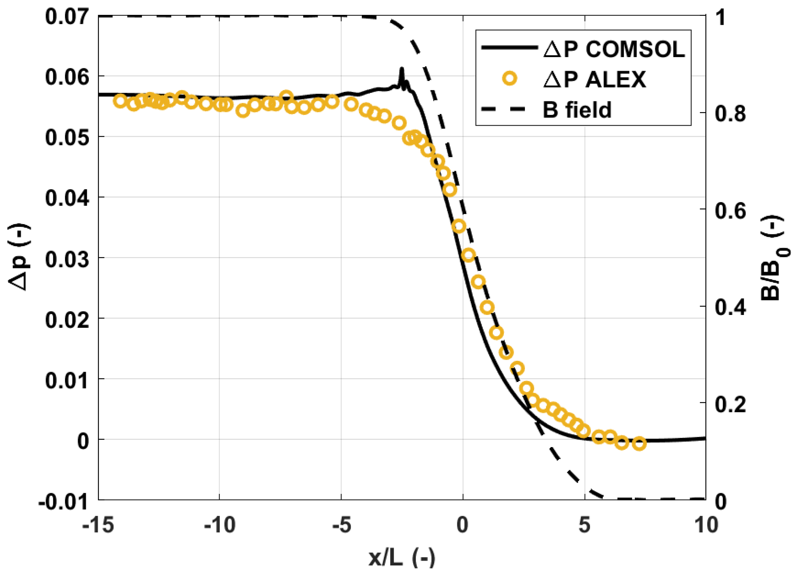
. The quantity selected for the comparison with the experimental results is the dimensionless axial pressure difference, that is, the pressure difference developed in the axis of the duct, scaled by σ U B 0 2 . The results are presented in Figure 2, where the magnetic field profile scaled by B 0 and the axial pressure difference obtained by Picologlou et al. [22] are shown in the present work. Good agreement between the curves can be appreciated. The biggest discrepancy appears in 5 < x / L < 0 , where COMSOL tends to overestimate the pressure difference. This behavior is also found in work by Sahu [8] and from the HIMAG Code calculations [26,27]. The difference between the two solutions is calculated using the integral of the curves with the following relation, called integral error index:
ε i n t = | 1 x m i n x m a x Δ p ( x ) d x x m i n x m a x Δ p A ( x ) d x |
where Δ p A (−) and Δ p (−) are, respectively, the ALEX experiment and the present work nondimensional axial pressure difference. The integrals are computed numerically, using the trapezoidal rule, and the resulting error is 1.10 % .

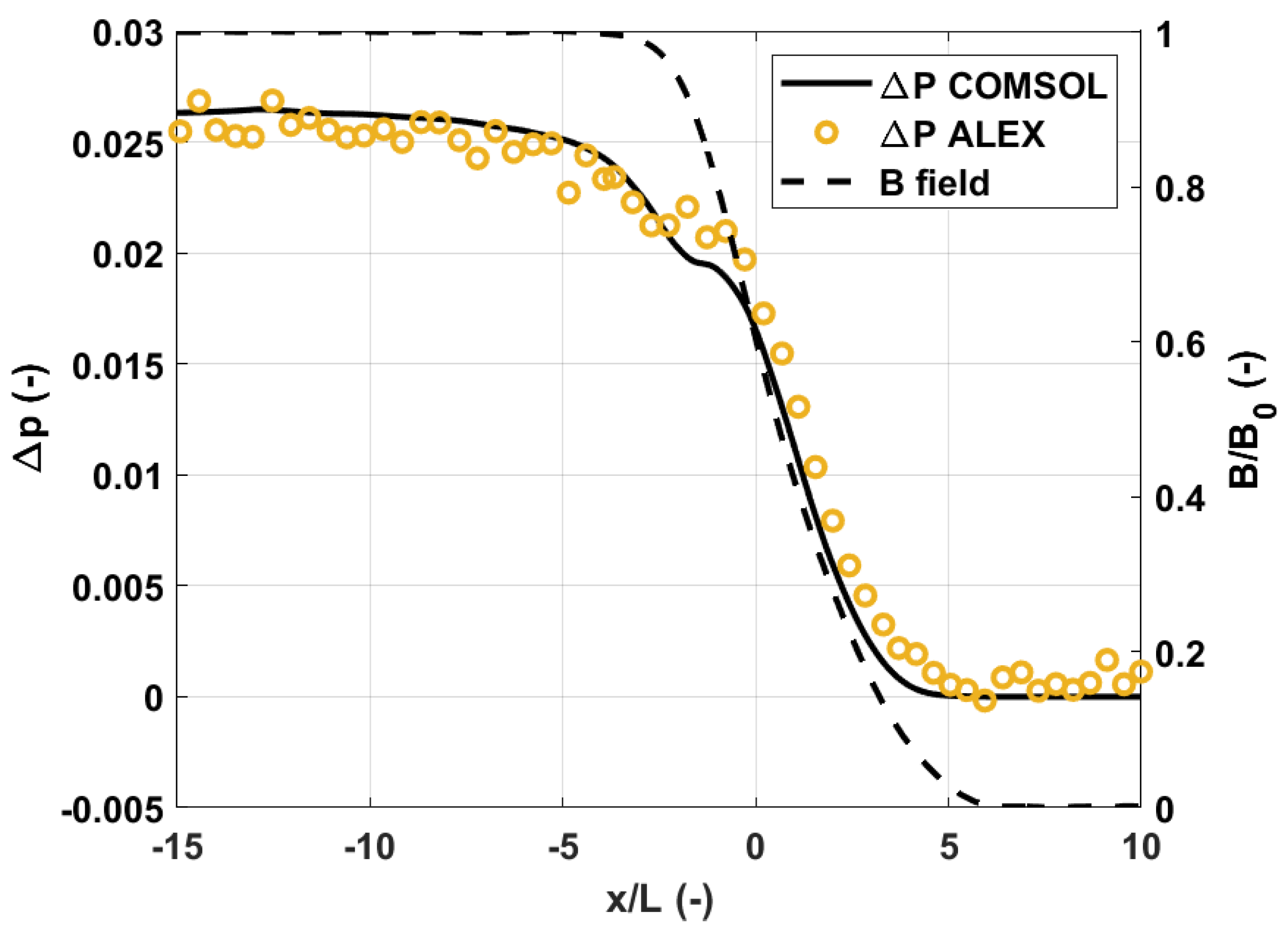
3.2.2. Circular Duct

In x -direction the mesh adopted is equivalent to the previous case, whereas, in the y and z plane, 25 boundary layers are considered, generated from the first layer of thickness 10 6 m, with a growth rate of 1.3. The total number of elements is 3.03 × 10 5 .
The parameters adopted for the study are H a = 6600 , N = 10,700 and c w = 0.027 . In Figure 3, the results are presented. The curves are matching very well, and the error is 0.913 % .

3.3. Magneto-Convection

The following benchmark cases were developed with the aim to include also representative cases for the liquid metals breeding blankets, such as the WCLL, being characterized by non-isothermal conditions and internal volumetric heating.
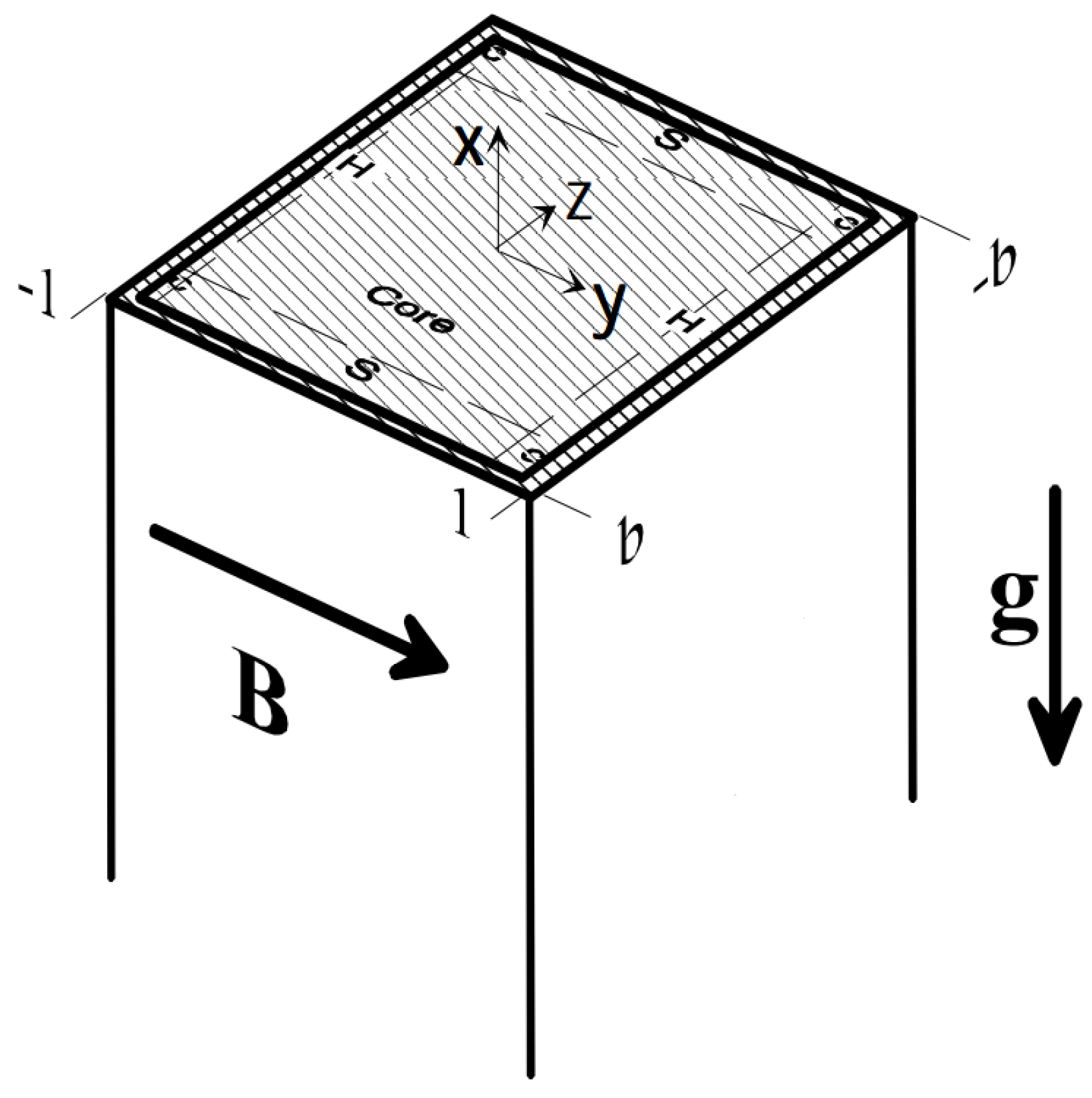
The flow of an electrically conducting fluid in a long vertical channel of the rectangular cross section was considered [16]. The flow is promoted by buoyancy forces arising from non-isothermal conditions; hence, we refer to this as magnetoconvection. With reference to Figure 4, the imposed magnetic field is B = B 0 y ^ and the gravitational acceleration g = g x ^ , with x ^ unit vector in x -direction, is aligned with the channel axis. Within this frame, two cases are considered: a differentially heated duct and a uniformly heated duct, solved by Di Piazza and Bühler [18] with the CFX commercial code (currently Ansys CFX). For both the problems, the Hartmann number is H a = 100 .
The problem is 2D, and the COMSOL solution is obtained for the nondimensional problem, expressed in depth in [28]. For the cases considered, G r H a 4 , from which results that the inertial term of the Navier–Stokes equation became negligible. The mesh adopted is analog to the one shown in Figure 1, where only one element is generated in the direction of g . The total number of elements for the mesh selected is 5120 , with 64 elements in the x -direction and 80 in the y -direction; eight cells were always ensured in the Hartmann and side layers. The velocity boundary conditions adopted in the study are non-slip at the duct walls and period flow conditions at the inlet–outlet. The electrical boundary condition is a thin wall condition on the walls. The temperature boundary conditions are defined, for the two different cases, in the next sub-sections.

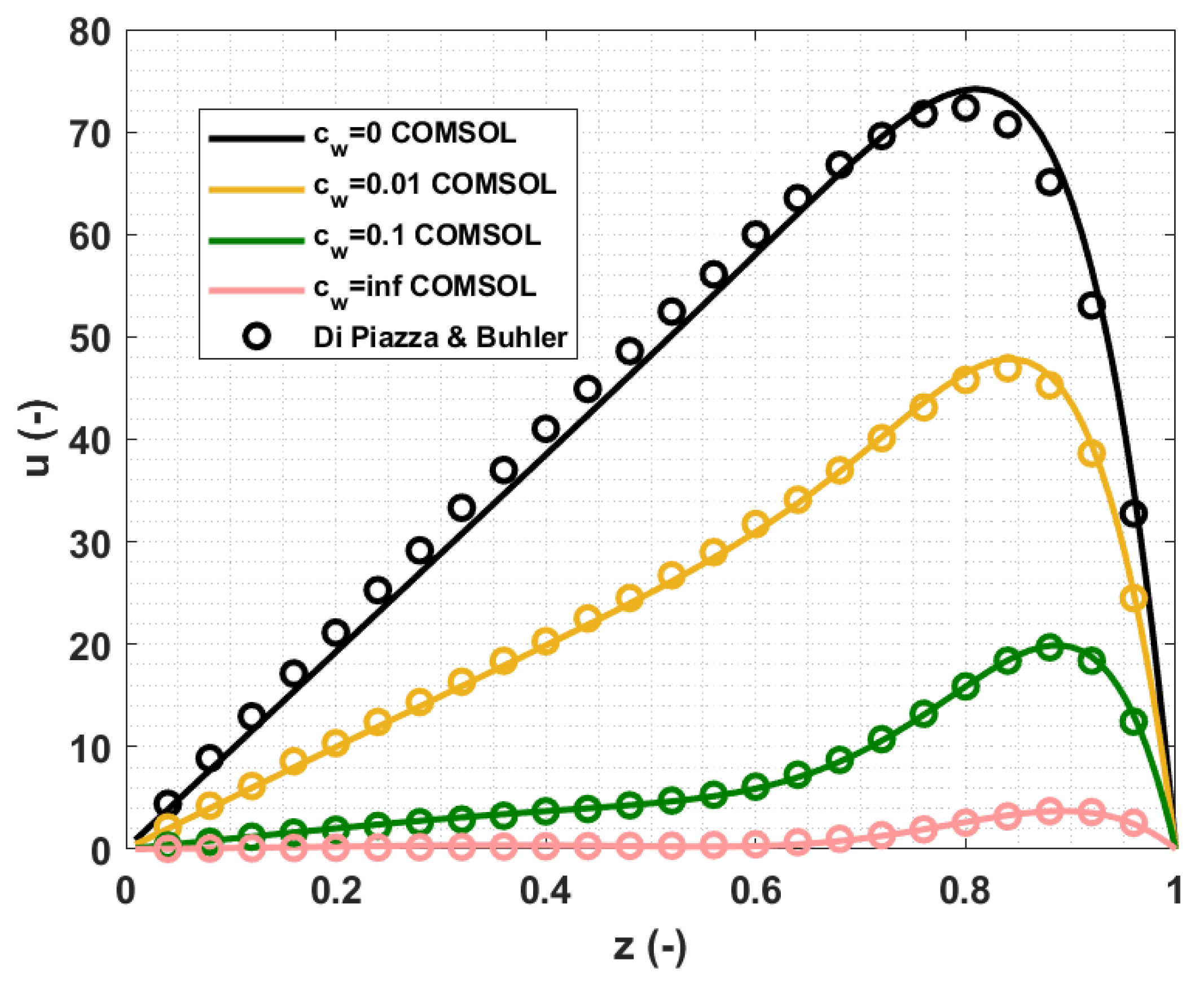
3.3.1. Differentially Heated Duct

The two boundaries placed in the side walls ( z = b and z = + b ) are kept at different temperatures, while the Hartmann walls are thermally insulated, and there is no internal heat generation.
A sensitivity analysis, with wall conductance ratio c w as a changing parameter, was carried out, and the nondimensional velocity profile at y = 0 as a function of z for half duct is shown in Figure 5 for H a = 100 .
It is interesting to notice that for the lower values of c w , the damping effect of magnetohydrodynamics is less evident, while in the core region, the solution is still dominated by buoyancy and Lorentz forces and exhibits a linear behavior, with a slope of H a for the perfectly insulating walls case [29]. In the lower conductivity cases, jets are not present. This is due to the fact that for low values of c w the side layer becomes better conducting than the side walls, and high current jets are now present in the layers parallel to the side walls. They are also parallel to B , so they do not interact with the magnetic field; therefore, the electromagnetic forces in the side layers become negligible, and the dominant effect is due to viscous dissipation.
For these cases, a comparison was made with respect to the numerical solutions [18] obtained with the CFX code. The integral of the curves is selected as a comparison parameter, and the relative difference is calculated with the integral error index:
ε i n t = | 1 z m i n z m a x u ( 0 , z ) d z z m i n z m a x u B ( 0 , z ) d z |
where u B ( 0 , z ) (−) is [18] x -direction dimensionless velocity profile and u ( 0 , z ) (−) is the current work profile, both taken at y = 0 . The error comparison is reported in Table 2. As can be appreciated, for all the cases, the maximum difference is lower than 2%.

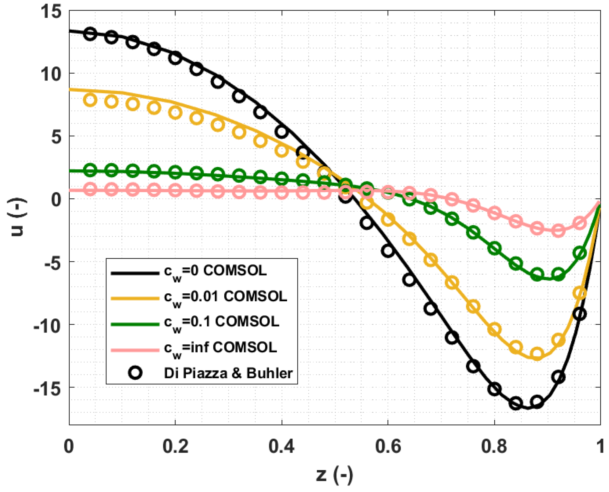
3.3.2. Uniformly Heated Duct

For the internally heated duct case, a volumetric heat generation Q ˙ is present, and the boundary at the side walls is kept at a fixed and equal temperature, while the Hartmann walls are thermally insulated.
The nondimensional velocity profiles at y = 0 and as a function of z -coordinate, a result of an analog sensitivity analysis to the one presented for the differentially heated duct case, are shown in Figure 6 for H a = 100 . For high wall conductivity ratios, the additional forces damp the velocity profile in the core region, and velocity jets are present in the side layers. For small values of c w , jets are no more present, and the solution at the side layers is dominated by viscous effects.
The error comparison is reported in Table 2, where the maximum difference is related to the analysis with c w = 0.01 , that, nevertheless, presents a value below 5%. It should be recalled that in both differentially heated duct and uniformly heated duct cases, the comparison was addressed on the numerical solutions of the codes.

3.4. Quasi-Two-Dimensional MHD Turbulent Flow

This case regards a quasi-two-dimensional MHD turbulent flow as proposed in [6]. Burr et al. [13] developed an experimental setup consisting of a rectangular stainless steel channel of side length 0.04 m and wall thickness 6 mm where the eutectic sodium–potassium alloy is circulated under the presence of a magnetic field. NaK, with density 865 kg m−3 and kinetic viscosity 9.5 × 10 7 m2 s−1, flows in the x -direction, and B is oriented in z and can be varied from 0.25 T to 2.5 T. The electric conductivity of the wall is   1.39 × 10 6 S m−1, whereas the one of the NaK is 2.8 × 10 6 S m−1, from which it results in wall conductance ratios of the side and Hartmann walls of c w , S = 0.0714 and c w , H = 0.0119 , respectively. The Hartmann numbers investigated are 600, 1200, 2400 and 4800 for Reynolds numbers between 3.3 × 10 3 and 1.0 × 10 5 .
The problem is solved numerically using a RANS k ε turbulence model that includes two transport equations for the turbulent kinetic energy k (m2 s−2) and for the dissipation of turbulent kinetic energy ε (m2 s−3). For k ε , Equation (2) becomes:
ρ u t + ρ ( u · ) u = p + ( μ + μ T ) 2 u + J × B 0
where μ T   [Pa s] is the eddy viscosity. The two closure equations of the model are:
( u · ) k = · [ ( μ + μ t σ k ) k ] + P k ρ ε + S k L
ρ ( u · ) ε = · [ ( μ + μ t σ ε ) ε ] + C ε 1 ε k P k C ε 2 ρ ε 2 k + S ε L
Here, P k (W m−3) is a source term, σ k (−), σ ε (−), C ε 1 (−) and C ε 2 (−) are turbulent model parameters. S k L (W m−3) and S ε L (W m−3) are source terms that include the damping of the turbulent kinetic energy and the dissipation of the turbulent kinetic energy due to the Lorentz force and were modeled by different authors [30,31,32]. The relations selected are the ones proposed by Meng et al. [14], expressed by the following equations:
S k L = σ B 2 k e C 1 M σ ρ B 2 ν k
S ε L = σ B 2 ε e C 1 M σ ρ B 2 ν k
where C 1 M (−) is a constant with value 30 , and ν (m2 s−1) is the kinematic viscosity. In these relations, σ / ρ B 2 ν / k is the characteristic turbulence damping time, and exp ( C 1 M σ / ρ B 2 ν / k ) is the decay rate of the turbulent kinetic energy.
The comparison parameters between Burr and the current study are the mean velocity profiles and turbulent kinetic energy of two-dimensional turbulence k 2 D (m2 s−2), defined as
k 2 D = 1 2 ( u 2 ¯ + w 2 ¯ )
where u (m s−1) and w (m s−1) are the fluctuating term of the velocity for the x -th and z -th components.
The mesh refinement was carried out until an appropriate wall lift-off in viscous units δ w + was obtained. In particular, δ w + = 11.06 for every case analyzed, that is the lower limit for COMSOL k ε turbulence model [33]. This value corresponds to the dimensionless wall distance y + , where the viscous sublayer meets the logarithmic layer. The total number of elements is 1.28 × 10 6 . The velocity boundary conditions adopted in the study are non-slip at the duct walls and imposed average velocity at the inlet. The electrical boundary condition is a thin wall condition on the walls.
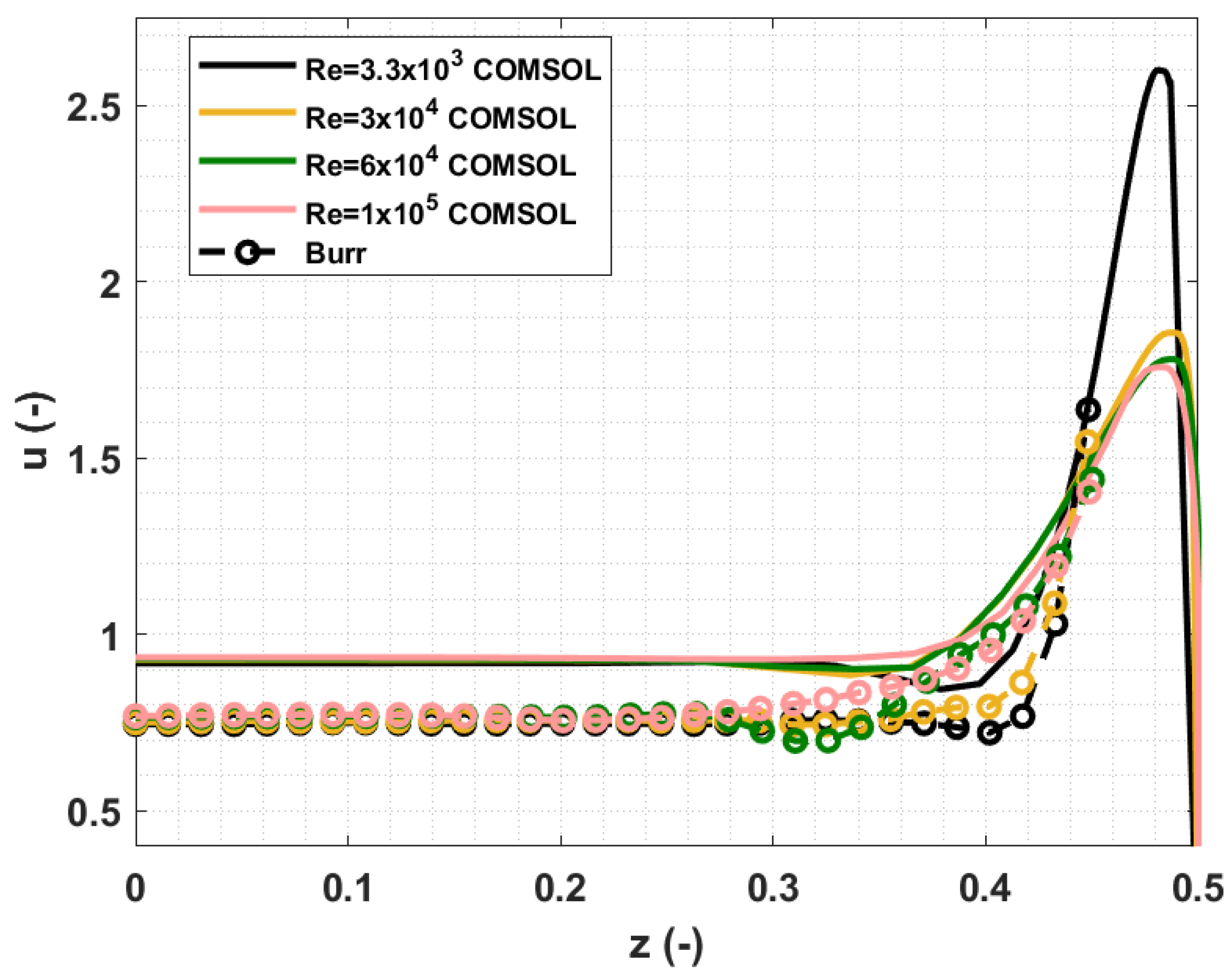
The mean velocity in x -direction u , calculated for H a = 4800 and various Reynolds numbers, is now compared with Burr results. In Figure 7, the COMSOL solutions and Burr experimental results are displayed.
The main characteristics of the flow are well expressed, and the influence of the Reynolds number on the flow is evident. This is a characteristic of turbulent MHD flows, while the velocity distribution of laminar MHD flows is governed only by H a . Turbulence smoothens out velocity peaks in the side walls that are reduced for increasing Reynolds numbers, and the width of the side layer increases with R e due to turbulent transfer of momentum.
In Table 3, the local relative errors between COMSOL and the experimental results, calculated with the following equation, are presented.
ε r e l = | 1 u / u e x p |
Here, u (−) is the x -direction velocity magnitude calculated with COMSOL code and u e x p (−) by the experiment, both evaluated at z = 0.45 , that is, the closest point to the side layer, obtained in the experiment. As it can be observed, values agree very well, with a maximum error of about 3.52 % . Comparing the velocity at z = 0 , there is a relative difference of about 12% between the numerical and experimental values. The code overestimated the bulk velocity, and the same behavior is reported in [14], which uses the same strategy to model the dissipation of the turbulent kinetic energy due to Lorentz forces.
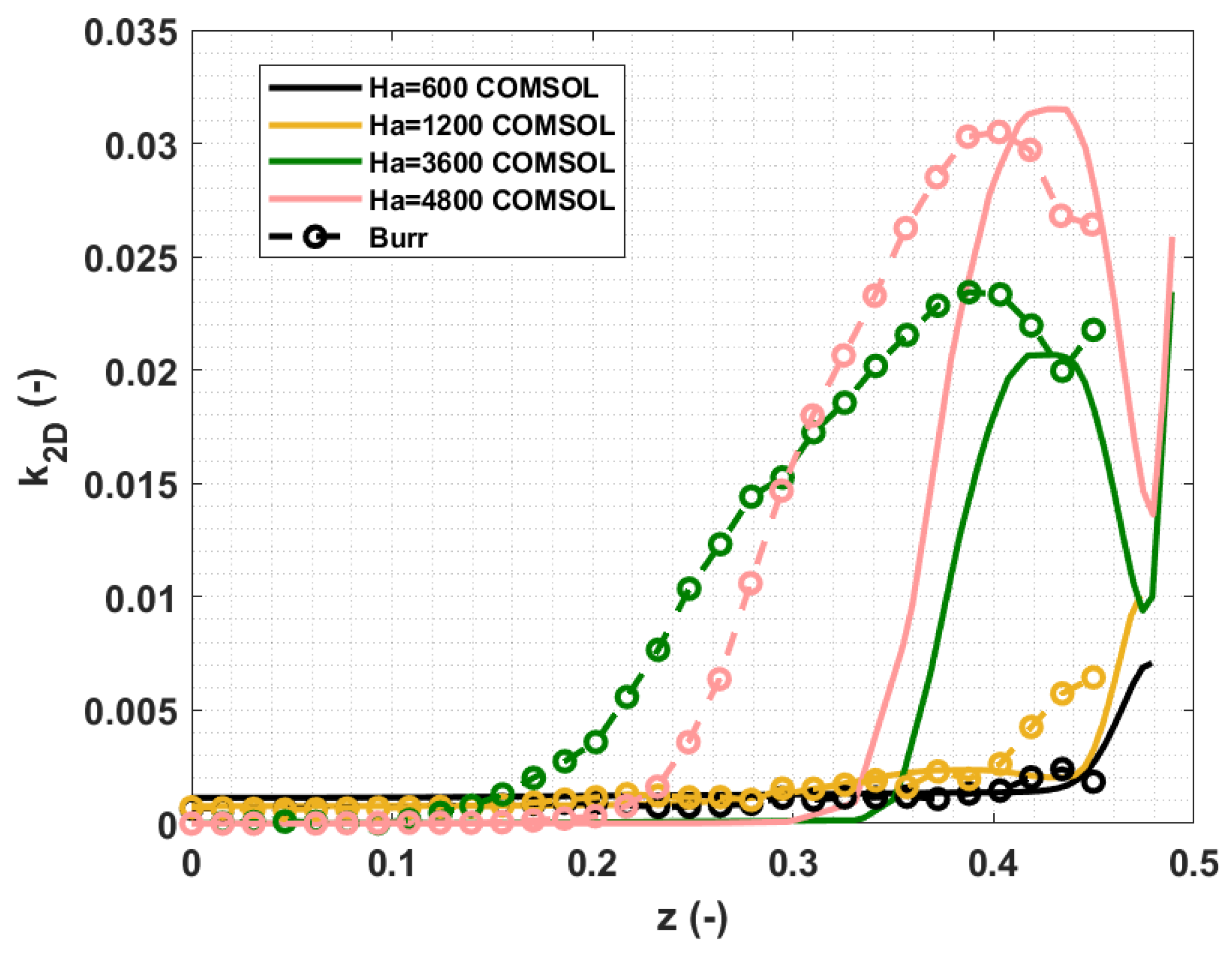
In Figure 8, the comparison between the distributions of the turbulent kinetic energy of two-dimensional turbulence k 2 D reported by Burr [13] and calculated with COMSOL are presented for R e = 1.0 × 10 5 and Hartmann numbers between 600 and 4800 . The values are captured along the z -axis at the midplane y = 0 . The increase in the turbulent kinetic energy as H a increases can be appreciated, proving that turbulence is promoted by the magnetic field. In both [14] and COMSOL results, turbulence is restrained to the side layers, decreasing fast moving towards the core region, where, in the experimental results, the flow, although weakly, remains turbulent. The anisotropicity of the turbulent flow is particularly evident for the high Hartmann number cases, where k 2 D k 3 D .
As shown by the results, the code can tackle quasi-two-dimensional MHD flow problems, giving reliable results, particularly in the side layer region. Further improvements are needed to better compute the bulk turbulence that is underestimated by the code.

3.5. Three-Dimensional Turbulent MHD Flow

The benchmark problem on 3D turbulent MHD flow addressed is the one proposed by Smolentsev et al. [6]. The eutectic GaInSn, with density 6360 kg m−3, the electrical conductivity of 3.46 × 10 6 S2 m−1 and kinetic viscosity of 3.4 × 10 7 m2 s−1, flows with a maximum flow rate of 2 × 10 3 m−3 s−1 in plexiglass (insulating) rectangular channel of length 0.5 m and 100 mm × 20 mm cross section, and starting from pure hydrodynamics conditions, is subjected to a nonuniform magnetic field generated by a magnetic obstacle. This is an experimental problem addressed by Andreev et al. [25]. The flow direction is x -oriented, and the magnetic field is in the z -direction. Starting from a zero value, the magnetic field monotonically increases until it reaches the maximum value of B 0 = 0.504   T at the center of the duct, corresponding to H a = 400 , then it decreases to zero. The magnetic field is slightly nonuniform also in the y -direction, but this feature is neglected in the COMSOL model. Further information on the B profile can be found in [25]. The Reynolds number selected is R e = 4000 ; therefore, the interaction parameter is equal to N = 40 .
The problem was solved using the Large Eddy Simulation (LES) model [34,35], as suggested by Smolentsev et al. [6]. In particular, the Residual Based Multiscale Variational (RBMV) method [16,34,35] was implemented. In this model, the velocity and pressure fields are decomposed into resolved and unresolved scales:
U = u + u
P = p + p
where u (m s−1) and u (m s−1) are the resolved scale and the unresolved scale velocities, respectively, and p (Pa) and p (Pa) are the resolved scale and the unresolved scale pressures. In the RBMV method, the unresolved velocity and pressure scales are modeled in terms of the equation residuals for the resolved scales. Further information on RBMV LES modeling can be found [33].
To ensure adequate space discretization, the resolution of wall layers was checked by u τ h w ν < 1 , where the left term is the dimensionless wall distance evaluated at the first mesh cell next to the wall. Here, u τ   is the friction velocity, h w is the thickness of the first mesh cell next to the wall,   ν is the kinematic viscosity. Time discretization was checked using the relation C = U Δ t h U < 0.5 , where C is the Courant number, with U flow velocity magnitude, Δ t time step and h U mesh size in the streamline direction. The total number of elements of the selected mesh is 1.8 × 10 6 . The velocity boundary conditions adopted in the study are non-slip at the duct walls and imposed average velocity at the inlet. The electrical boundary condition is a thin wall condition on the walls.
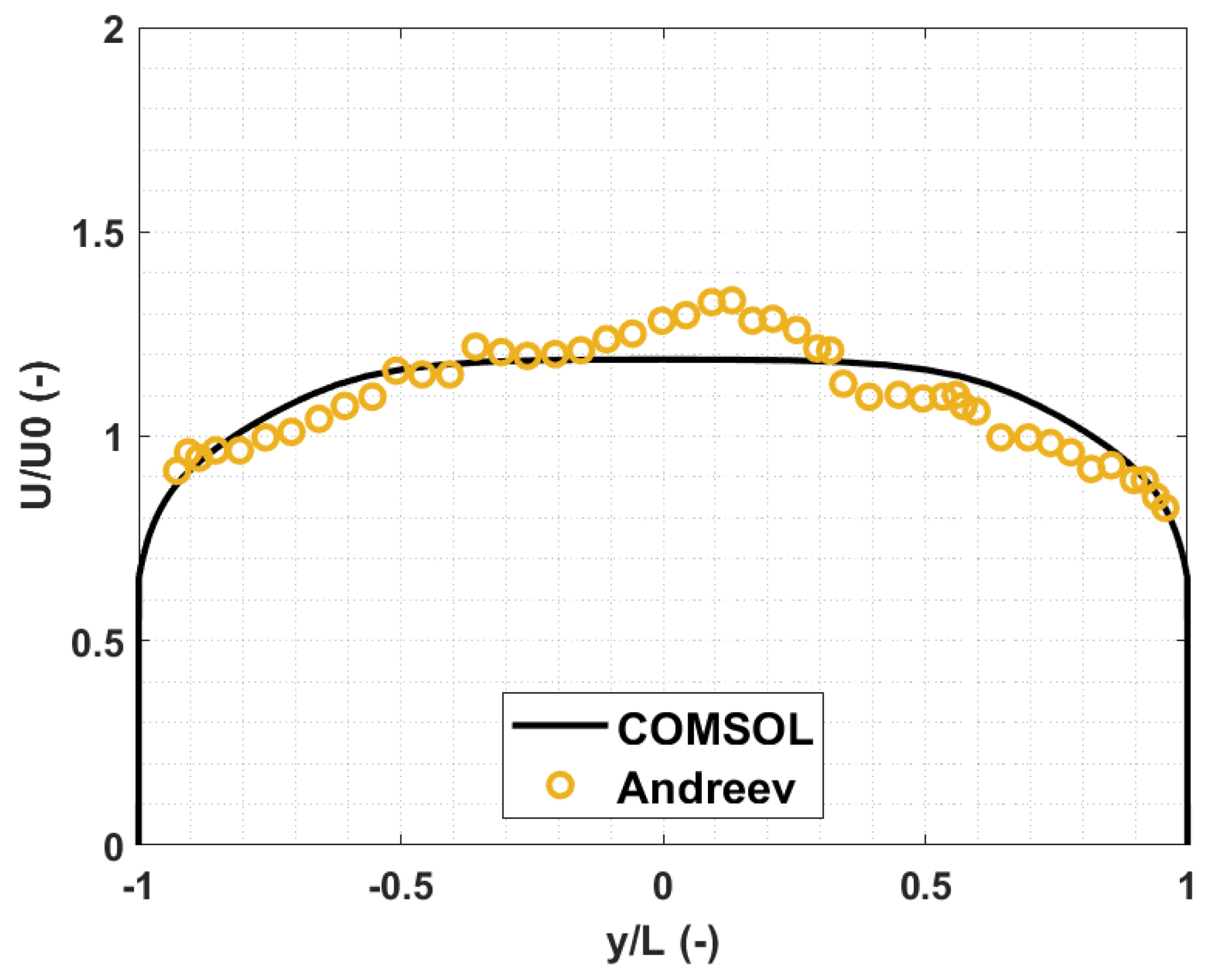
The selected comparison parameter is the mean velocity profile and the mean electric potential, evaluated at different distances along the channel. In particular, the selected locations correspond to the main flow regions, as described by Andreev. In Figure 9, a comparison between COMSOL and Andreev’s velocity profile at x H = 5.3 , with H channel height in z -direction, is presented.
The profile is referred to as the first region indicated by the author, characterized by the increasing magnetic field that influences the flow and damps its perturbations, called “turbulence suppression region”. As evident, the agreement between the curves is good, and the integral error index is
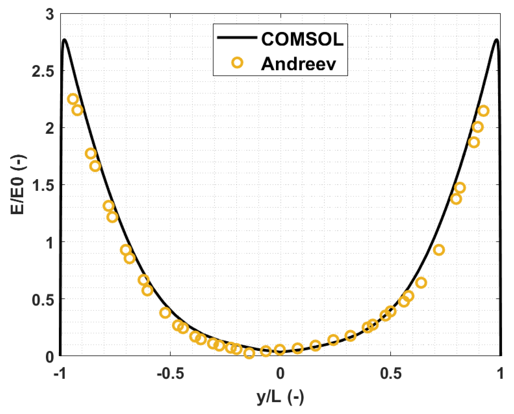
 0.947 % . In Figure 10, the electric potential profile, placed at x H = 0 , is shown.
This region, around the center of the duct where B is maximum, is called “vortical region”. The magnetic field suppresses the fluctuations in the direction parallel to the magnetic field, and the flow becomes quasi-two-dimensional. The integral error index is
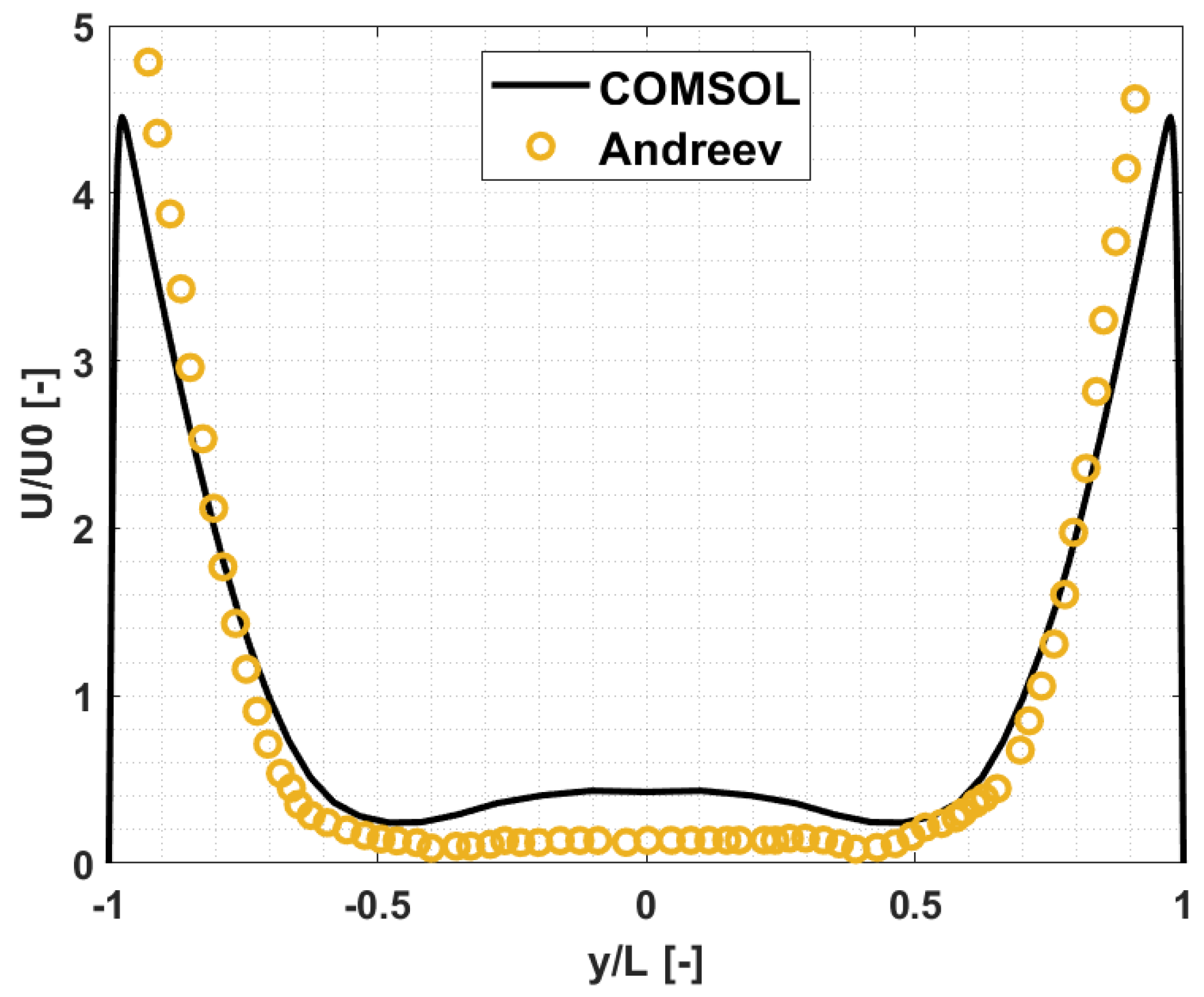
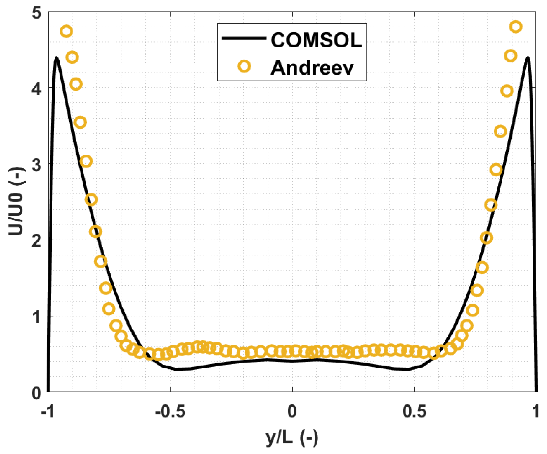
 4.21 % . In Figure 11 and Figure 12, the results for the last region, named “wall jet region”, are reported.
This region is located on the remaining part of the channel, where the magnetic field decreases. As observable, the velocity in the middle plane increases greatly, going from x / H = 3 to x / H = 6 thanks to the drop of the intensity of the magnetic field, and the quasi-two-dimensional profile stretches to the core of the flow. The agreement between the velocity fields is quite good, and the relative errors in percentage are 6.72 % at x / H = 3 and 7.81 % at x / H = 6 .
As presented, the code is capable of representing the characteristic regions of the experimental problem, and the errors obtained are, for every case, well below 10 % . The results are summarized in Table 4, and they provide confidence in the capabilities of COMSOL to simulate fully 3D turbulent flows.

4. Discussion

In this paper, a verification and validation procedure was followed, as proposed by Smolentsev et al. [6], and different liquid metal MHD problems were solved, with the aim of verifying the developed models using the commercial software COMSOL Multiphysics. For the magnetoconvection case, the considered benchmarks were the ones tackled by Di Piazza and Bühler [18], presenting the typical conditions that are expected in liquid metal breeding blankets.
The compared parameters showed great agreement for laminar flow problems, both isothermal and non-isothermal. As far as the turbulent cases are concerned, Q2D and 3D, a modified version of the RANS k ε and the LES RBMV models were adopted, respectively, and the deriving results, in terms of relative errors and the capability of describing the flow features, are very promising.

Author Contributions

Conceptualization, C.A., L.C. and R.T.; methodology, C.A.; software, C.A.; validation, C.A.; formal analysis, C.A.; investigation, C.A.; data curation, C.A.; writing—original draft preparation, C.A.; writing—review and editing, C.A., L.C. and R.T.; supervision, R.T., M.U. and M.Z. All authors have read and agreed to the published version of the manuscript.

Funding

This work has been carried out within the framework of the EUROfusion Consortium and has received funding from the Euratom research and training programme 2014–2018 and 2019–2020 under grant agreement No 633053. The views and opinions expressed herein do not necessarily reflect those of the European Commission.

Institutional Review Board Statement

Not applicable.

Informed Consent Statement

Not applicable.

Data Availability Statement

The study didn’t report and data.

Conflicts of Interest

The authors declare no conflict of interest.

References

  1. Del Nevo, A.; Arena, P.; Caruso, G.; Chiovaro, P.; Di Maio, P.; Eboli, M.; Edemetti, F.; Forgione, N.; Forte, R.; Froio, A.; et al. Recent progress in developing a feasible and integrated conceptual design of the WCLL BB in EUROfusion project. Fusion Eng. Des. 2019, 146, 1805–1809. [Google Scholar] [CrossRef] [Green Version]
  2. Miyazaki, K.; Inoue, S.; Yamaoka, N. MHD Pressure Drop of Liquid Metal Flow in Circular and Rectangular Ducts under Transverse Magnetic Field. In Liquid Metal Magnetohydrodynamics, 2nd ed.; Springer: Dordrecht, The Netherlands, 1989; Volume 10, pp. 29–36. [Google Scholar] [CrossRef]
  3. Candido, L.; Testoni, R.; Utili, M.; Zucchetti, M. Tritium transport model at breeder unit level for WCLL breeding blanket. Fusion Eng. Des. 2019, 146, 1207–1210. [Google Scholar] [CrossRef]
  4. Alberghi, C.; Candido, L.; Testoni, R.; Utili, M.; Zucchetti, M. Magneto-convective effect on tritium transport at breeder unit level for the WCLL breeding blanket of DEMO. Fusion Eng. Des. 2019, 146, 2319–2322. [Google Scholar] [CrossRef]
  5. Candido, L.; Alberghi, C.; Moro, F.; Noce, S.; Testoni, R.; Utili, M.; Zucchetti, M. A novel approach to the study of magnetohydrodynamic effect on tritium transport in WCLL breeding blanket of DEMO. Fusion Eng. Des. 2021, 167, 112234. [Google Scholar] [CrossRef]
  6. Smolentsev, S.; Badia, S.; Bhattacharyay, R.; Bühler, L.; Chen, L.; Huang, Q.; Jin, H.-G.; Krasnov, D.; Lee, D.-W.; Valls, E.M.D.L.; et al. An approach to verification and validation of MHD codes for fusion applications. Fusion Eng. Des. 2015, 100, 65–72. [Google Scholar] [CrossRef] [Green Version]
  7. Kim, S.; Kim, M.; Lee, D.; Choi, C. Code validation and development for MHD analysis of liquid metal flow in Korean TBM. Fusion Eng. Des. 2012, 87, 951–955. [Google Scholar] [CrossRef]
  8. Sahu, S.; Bhattacharyay, R. Validation of COMSOL code for analyzing liquid metal magnetohydrodynamic flow. Fusion Eng. Des. 2018, 127, 151–159. [Google Scholar] [CrossRef]
  9. Yan, Y. Validation of COMSOL Multiphysics for magneto-hydro-dynamics (MHD) flows in fusion applications. In Proceedings of the COMSOL Conference, Boston, MA, USA, 5 October 2017. [Google Scholar]
  10. Feng, J.; Chen, H.; He, Q.; Ye, M. Further validation of liquid metal MHD code for unstructured grid based on OpenFOAM. Fusion Eng. Des. 2015, 100, 260–264. [Google Scholar] [CrossRef]
  11. He, Q.; Chen, H.; Feng, J. Acceleration of the OpenFOAM-based MHD solver using graphics processing units. Fusion Eng. Des. 2015, 101, 88–93. [Google Scholar] [CrossRef]
  12. Gajbhiye, P.; Throvagunta, P.; Eswaran, V. Validation and verification of a robust 3-D MHD code. Fusion Eng. Des. 2018, 128, 7–22. [Google Scholar] [CrossRef]
  13. Burr, U.; Barleon, L.; Muller, U.; Tsinober, A. Turbulent transport of momentum and heat in magnetohydrodynamic rectangular duct flow with strong sidewall jets. J. Fluid Mech. 2000, 406, 247–279. [Google Scholar] [CrossRef]
  14. Meng, Z.; Zhang, S.; Jia, J.; Chen, Z.; Ni, M. A K-Epsilon RANS turbulence model for incompressible MHD flow at high Hartmann number in fusion liquid metal blankets. Int. J. Energy Res. 2018, 42, 314–320. [Google Scholar] [CrossRef]
  15. Bazilevs, Y.; Calo, V.; Cottrell, J.; Hughes, T.J.R.; Reali, A.; Scovazzi, G. Variational multiscale residual-based turbulence modeling for large eddy simulation of incompressible flows. Comp. Meth. Appl. Mech. Eng. 2007, 197, 173–201. [Google Scholar] [CrossRef]
  16. Liu, J. Residual-Based Variational Multiscale Models for the Large Eddy Simulation of Compressible and Incompressible Turbulent Flows. Ph.D. Thesis, Rensselaer Polytechnic Institute, Troy, NY, USA, 2012. [Google Scholar]
  17. Volker, J.; Songul, K. A finite element variational multiscale method for the Navier-Stokes equations. SIAM J. Sci. Comp. 2005, 26, 1485–1503. [Google Scholar] [CrossRef]
  18. Di Piazza, I.; Bühler, L. Numerical Simulations of Buoyant Magnetohydrodynamic Flows Using the CFX Code; Furschungszentrum Karlsruhe GmbH: Karlsruhe, Germany, 1999. [Google Scholar]
  19. Davidson, P.A. An Introduction to Magnetohydrodynamics, 1st ed.; Cambridge University Press: Cambridge, UK, 2001. [Google Scholar] [CrossRef]
  20. Shercliff, J.A. Steady motion of conducting fluids in pipes under transverse magnetic fields. Math. Proc. Camb. Philos. Soc. 1953, 49, 136–144. [Google Scholar] [CrossRef]
  21. Hunt, J.C.R. Magnetohydrodynamic flow in rectangular ducts. J. Fluid Mech. 1965, 21, 577–590. [Google Scholar] [CrossRef]
  22. Picologlou, B.F.; Reed, C.B. Experimental investigation of 3-D MHD flows at high Harmann numbers and interaction parameters. In Liquid Metal Magnetohydrodynamics, 2nd ed.; Springer: Dordrecht, The Netherlands, 1989; Volume 10, pp. 71–77. [Google Scholar] [CrossRef]
  23. Reed, C.B.; Picologlou, B.F.; Dauzvardis, P.V. Experimental facility for studying MHD effects in liquid metal. Fusion Tech. 1985, 8, 257–263. [Google Scholar] [CrossRef]
  24. Reed, C.B.; Picologlou, B.F.; Hua, T.Q.; Walker, J.S. ALEX results: A comparison of measurements from a round and a rectangular duct with 3-D code predictions. In Proceedings of the Symposium on Fusion Engineering, Monterey, CA, USA, 12–16 October 1987. [Google Scholar]
  25. Andreev, O.; Kolesnikov, Y.; Thess, A. Experimental study of liquid metal channel flow under the influence of a nonuniform magnatic field. Phys. Fluids 2006, 18, 065108. [Google Scholar] [CrossRef] [Green Version]
  26. Ni, M.-J.; Munipalli, R.; Huang, P.; Morley, N.B.; Abdou, M.A. A current density conservative scheme for incompressible MHD flows at a low magnetic Reynolds number. Part II: On an arbitrary collocated mesh. J. Comp. Phys. 2007, 227, 205–228. [Google Scholar] [CrossRef]
  27. Munipalli, R.; Shankar, V.; Ni, M.-J.; Morley, N. Development of a 3-D incompressible free surface MHD computational environment for arbitrary geometries: HIMAG. In DOE Phase-II SBIR Final Report; DOE: Washington, DC, USA, 2003. [Google Scholar]
  28. Buhler, L. Laminar buoyant magnetohydrodynamic flow in vertical rectangular ducts. Phys. Fluids 1998, 10, 223–236. [Google Scholar] [CrossRef]
  29. Bojarevics, V. Buoyancy driven flow and its stability in a horizontal rectangular channel with an arbitrary oriented transversal magnetic field. Magnetohydrodynamics 1996, 31, 245–253. [Google Scholar]
  30. Ni, H.C.; Gradner, R.A. Numerical analysis of turbulent pipe flow in a transfer magnetic field. Int. J. Heat Mass Transf. 1997, 40, 1839–1851. [Google Scholar] [CrossRef]
  31. Kenjeres, S.; Hanjalic, K. On the implementation of effects of Lorentz force in turbulence closure models. J. Heat Fluid Flow 2000, 21, 329–337. [Google Scholar] [CrossRef]
  32. Smolentsev, S.; Abdou, M.; Morley, N.; Ying, A.; Kunugi, T. Application of the "K-eps" model to open channel flows in a magnetic field. Int. J. Eng. Sci. 2002, 40, 693–711. [Google Scholar] [CrossRef]
  33. COMSOL Multiphysics User Guide. Available online: https://doc.comsol.com/5.5/doc/com.comsol.help.comsol/COMSOL_ReferenceManual.pdf (accessed on 21 July 2021).
  34. Chapman, D.R. Computational Aerodynamics Development and Outlook. AIAA J. 1979, 17, 1293–1313. [Google Scholar] [CrossRef]
  35. Choi, H.; Moin, P.A. Grid-point requirements for large eddy simulation: Chapman’s estimates. Phys. Fluids 2012, 24, 011702. [Google Scholar] [CrossRef]
Figure 1. Example of mesh adopted for Shercliff’s and Hunt’s cases, corresponding to H a = 5000 . The elements are distributed, increasing the cell size moving inward to the duct.
Energies 14 05413 g001
Figure 2. Comparison of the COMSOL code results against ALEX experiment at Argonne National Laboratory [22], rectangular duct.
Energies 14 05413 g002
Figure 3. Comparison of the COMSOL code results against ALEX experiment at Argonne National Laboratory [22], circular duct.
Energies 14 05413 g003
Figure 4. Geometry sketch for the two benchmark cases related to magneto-convective motion.
Energies 14 05413 g004
Figure 5. Numerical solutions of differentially heated duct case from [18] and from the COMSOL model.
Energies 14 05413 g005
Figure 6. Numerical solutions of uniformly heated duct case from [18] and from the COMSOL model.
Energies 14 05413 g006
Figure 7. Comparison of the numerical results against Burr experiment [13]. Mean velocities at the midplane y = 0 for H a = 4800 .
Energies 14 05413 g007
Figure 8. Comparison of the numerical results against Burr experiment [13]. Turbulent kinetic energy of two-dimensional turbulence k 2 D at the midplane y = 0 for   R e = 1.0 × 10 5 .
Energies 14 05413 g008
Figure 9. Comparison of the numerical results against Andreev experiment [25]. Velocity profile at z / H = 0 and x / H = 5 / 3 (turbulence suppression region).
Energies 14 05413 g009
Figure 10. Comparison of the numerical results against Andreev experiment [25]. Electric potential profile at z / H = 0 and x / H = 0 (vortical region).
Energies 14 05413 g010
Figure 11. Comparison of the numerical results against Andreev experiment [25]. Velocity profile at z / H = 0 and x / H = 3 (wall jet region).
Energies 14 05413 g011
Figure 12. Comparison of the numerical results against Andreev experiment [25]. Velocity profile at z / H = 0 and x / H = 6 (wall jet region).
Energies 14 05413 g012
Table 1. Comparison between the results of Shercliff’s case and Hunt’s case for 2D fully developed laminar steady flow. Results in terms of Q ˜ (−).
Shercliff Case
H a (−) Analytical   Q ˜ (−) COMSOL   Q ˜ (−) ε r e l (%)
500 7.680 × 10 3 7.690 × 10 3 0.130
5000 7.902 × 10 4 7.906 × 10 4 0.0456
10,000 3.965 × 10 4 3.946 × 10 4 0.478
15,000 2.648 × 10 4 2.660 × 10 4 0.453
Hunt Case
H a (−) Analytical   Q ˜ (−) COMSOL   Q ˜ (−) ε r e l (%)
500 1.405 × 10 3 1.406 × 10 3 0.0356
5000 1.907 × 10 5 1.904 × 10 5 0.184
10,000 5.169 × 10 6 5.163 × 10 6 0.118
15,000 2.425 × 10 6 2.410 × 10 6 0.635
Table 2. Comparison between COMSOL code and Di Piazza and Buhler solutions for H a = 100 . Results in terms of integral error index.
Differentially Heated DuctUniformly Heated Duct
c w   ( ) ε r e l   ( % ) ε r e l   ( % )
0 0.957 1.50
0.01 0.326 4.78
0.1 1.77 0.585
1.36 0.770
Table 3. Local error for the quasi-two-dimensional turbulent flow for H a = 4800 and different R e . Results in terms of u   ( ) .
R e (−) Experimental   u (−) COMSOL   u (−) ε r e l (%)
3.3 · 10 3 1.638 1.644 0.368 %
3 · 10 4 1.547 1.492 3.52 %
6 · 10 4 1.442 1.482 3.31 %
1 · 10 5 1.405 1.447 2.98 %
Table 4. Comparison between COMSOL code and [25] experiment. Results in terms of integral error index.
x / H (−) 5.3 0 3 6
ε r e l (%) 0.947 % 4.21 % 6.72 % 7.81 %
Publisher’s Note: MDPI stays neutral with regard to jurisdictional claims in published maps and institutional affiliations.

