Abstract
This article presents a numerical model of an aeronautical hybrid electric propulsion system (HEPS) based on an energy method. This model is designed for HEPS with a total power of 100 kW in a parallel configuration intended for ultralight aircraft and unmanned aerial vehicles (UAV). The model involves the interaction between the internal combustion engine (ICE), the electric motor (EM), the lithium battery and the aircraft propeller. This paper also describes an experimental setup that can reproduce some flight phases, or entire missions, for the reference aircraft class. The experimental data, obtained by reproducing two different take-offs, were used for model validation. The model can also simulate anomalous operating conditions. Therefore, the tests chosen for the model validation are characterized by the EM flux weakening (“de-fluxing”). This model is particularly suitable for preliminary stages of design when it is necessary to characterize the hybrid system architecture. Moreover, this model helps with the choice of the main components (e.g., ICE, EM, and transmission gear ratio). The results of the investigation conducted for different battery voltages and EM transmission ratios are shown for the same mission. Despite the highly simplified model, the average margin of error between the experimental and simulated results was generally under 5%.
1. Introduction
Air travel is continuing to experience the fastest growth among all modes of transportation, therefore, environmental issues such as noise, emissions, and fuel consumption are becoming important for energy and environmental sustainability [1].High concentrations of air pollutants (e.g., PM2.5, black carbon, CO, NOx) are observed around general aviation airports, with potential health implications for persons living nearby [2]. Recent studies carried out on a population of air transport workers show a statistically significant impact on the risk of contracting cancer [3]. The latter, in fact, are often exposed to various chemical and physical dangers (e.g., jet engine emissions, ionizing radiation, electromagnetic fields from cockpit instruments, ultraviolet radiation, etc.).
Much research in the aeronautical field aims to support natural resources by saving emissions; of all the systems, the full electric propulsion system (FEPS) and the hybrid electric propulsion system (HEPS) [4] seem to have a primary role in the sustainable development of general aviation, and for ultralight aircraft, and UAV [5].
These propulsion systems ensure not only a reduction in noise and exhaust gas emissions, but due to their internal combustion engines, they also offer greater mission flexibility with a potential increase in overall efficiency [6,7].
Glassock et al. [6] showed that a short-duration mission such as skydiving equipped with a hybrid propulsion system can contribute to fuel reduction.
Xie et al. [8] developed a simplified model of a HEPS, demonstrating that such application on a UAV achieved a fuel saving of around 7% when it was compared with conventional ICE propulsion.
FEPS are more environmentally friendly than HEPS, however, the energy density (or specific energy) of the electrical energy storage source, such as batteries, is much lower than fossil fuels. Therefore, the aircraft that use FEPS are unlikely to achieve the same distances as aircraft powered by conventional engines. HEPS can be employed today as a transition technology, which guarantees greater autonomy of the FEPS by reducing emissions and noise (e.g., range extender). Moreover, the HEPS could establish a bridge between conventional and new certification standards for fully electric aircraft.
For these reasons, HEPSs are attracting great interest in regard to aeronautical applications. Many multidisciplinary HEPS-focused models are available in the literature, each developed with a different orientation focus, and tools.
Some studies are focused on aircraft dynamics and flight missions, such as [6,9,10]. Among them, Glassock et al. [6] developed his model with reference to an aircraft of 2700–3500 kg for an installed power of 670 kW. Sliwinski et al. [9] and Narum et al. [10] studied, in more detail, unmanned aircraft with installed power below 2 kW. Interesting developments in aircraft dynamics on-line management can be derived from artificial intelligence studies. Some studies have already applied this technique to autonomous unmanned vehicles (e.g., Sands [11]).
Other works are oriented to energy management strategies [12,13,14]. In particular, Bongermino et al. [12] analyzed an HEPS composed of a Wankel engine and a permanent magnet-assisted synchronous reluctance motor. The model proposed the use of the data on a known mission as input. On the contrary, Xie et al. [13] developed an energy management strategy that does not require knowledge of the entire mission. Its approach is instantaneous and based on fuzzy logic algorithms. Zhang et al. [14] also developed an energy management strategy based on fuzzy logic, however, its hybrid system is composed of a photovoltaic panel, a fuel cell and a LiPo battery.
Finally, many works present a specific model for engine simulation. Cameretti et al. [15] analyzed a solution with a turboprop coupled to a permanent magnet synchronous motor (PMSM) with a total installed power of about 1400 kW (in parallel configuration). Both the engine and battery were characterized analytically.
Xie et al. [8] presented a model validated on a parallel HEPS with 25 kW ICE and 110 kW PSMS. Both engines were characterized through analytical functions with regard to performance (torque-RPM), while consumption and efficiencies were included as maps. The batteries were modelled analytically.
Hung et al. [16] presented a planetary gearbox to couple EM, ICE, and the propeller for aircraft with 4 kW of maximum power. The ICE and the EM were entirely modelled using maps, while the battery and transmission were modelled analytically.
The model developed by Frosina et al. [17] was developed in the AMESim® (Siemens PLM Software, Plano, TX, USA) environment for aircraft with 130 kW of maximum power. The EM was modelled in detail with analytical sub-models presented in the libraries of the environment. The ICE was modelled through maps of performance, consumption, and emissions.
This work proposes a model, developed in the MATLAB/Simulink® (R2017b MathWorks, Inc., Natick, MA, USA) environment, validated with experimental tests, and designed for a parallel HEPS with PMSM, suitable for the 100 kW aircraft category.
The main features of the model are:
- High versatility, which is linked to the setup of the components chosen from libraries defined based on commercial datasheets;
- Speed of calculation;
- Follows time-varying dynamics;
- Complex missions can be evaluated.
Therefore, the model is useful in the preliminary dimensioning phase, in particular, it is possible to change the principal components (e.g., ICE, EM, battery, gear ratio) to find the best solution in terms of maximum propulsion power, weight estimation and avoiding operating zone.
2. Materials and Methods
2.1. Experimental Setup and Method
In a hybrid electric propulsion system, two or more power sources are combined to increase the system overall efficiency. The most common hybrid configurations are the series, the parallel and the series-parallel. Among them, the one chosen for this application was the parallel configuration, which allows the summing of the power of the ICE and the EM so that the EM can be smaller than in the series configuration. Moreover, parallel hybrid systems can operate with only one power source active (ICE or EM), with both active, and with the EM in generator mode.
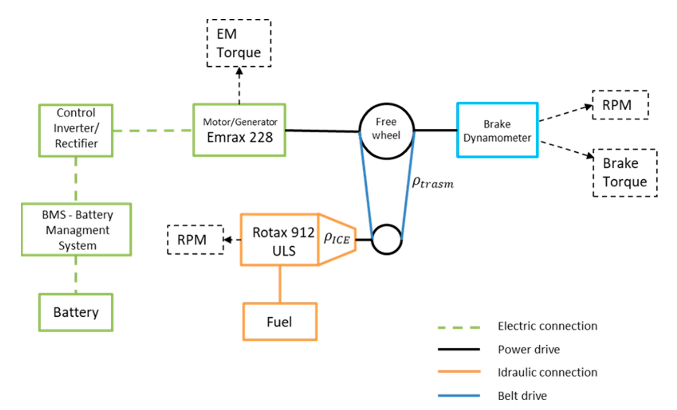
The main parts of the examined HEPS are the ICE, the EM, the batteries, and the mechanical drive. Figure 1 shows the HEPS scheme examined in this work.
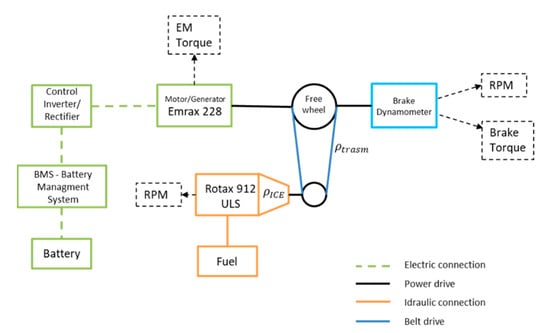
Figure 1.
Parallel hybrid propulsion system adopted scheme.
The ICE employed was the aeronautic, spark ignition, four-stroke engine Rotax® 912 ULS (BRP-Rotax Gmbh & co. KG, Gunskirchen, Austria) with an integrated gear box, . It is a four-cylinder boxer engine with two spark plugs for each cylinder. Its total capacity is 1354 cm3. Its maximum power is 73.5 kW at 5800 RPM and its maximum torque is 128 Nm at 5100 RPM. The EM (motor/generator) employed was the permanent magnet synchronous motor (PMSM) Emrax® 228 (EMRAX d.o.o. Molkova pot 5SI-1241 Kamnik Slovenia) low voltage. It has a maximum continuous power of 50 kW at 5500 RPM and maximum torque of 96 Nm. This data refers to the liquid cooled configuration, which has performances 15% lower than the Combined Cooled version. The employed battery pack is based on Li-ion cells. It has a nominal voltage of 74 V and a capacity of 3 kWh (~40 Ah).
The ICE transmits its torque to the propeller shaft through a toothed transmission belt. The speed reduction ratio is . The overall speed reduction ratio from the crankshaft ICE to the propeller-shaft is . The EM is on the propeller shaft.
A freewheel allows the power transmission across the shafts. A freewheel is a mechanism that allows the torque to be transmitted only one way. It is based on angular speed variations. This solution has also been proposed by Machado et al. [18], although for a smaller application (the overall power was less than 4 kW).
The HEPS was installed in an engine test room to perform the experimental tests. An eddy current brake simulated the propeller resistant torque. The brake was controlled by a dedicated electronic device that regulated the brake currents to meet the requested torque or speed setpoint. The brake was provided with a load cell and a variable reluctance sensor to measure the actual torque and speed.
The EM stator was fixed on an oscillating casing, which was constrained through a load cell. This solution allows the measurement of the EM torque.
Table 1 summarizes the HEPS main components.

Table 1.
HEPS equipment.
Table 2 shows the sensors employed in the acquisition system. This system is based on the National Instrument Acquisition Board NI cFP 1808, and it is managed by a dedicated software written in LabView® (15.0, Austin, TX, USA) environment.
Table 2.
Measurement sensors.
A feedback loop controller drives the dynamometer brake. The controller has different functioning modes. Among them, there is the quadratic load function, which sets the brake torque proportionally to the square of the rotational speed. This mode is usually used to test marine and aeronautical ICEs, as that kind of control simulates the propellers load in quasi-static translations. The brake was set to keep the system speed below 2700 RPM. The resulting quadratic function was calculated ex-post from the torque and speed measurements (see also Section 2.2.4).
Two experimental runs were performed to validate the model. Both tests were performed with the initial battery state of charge (SOC) at 50% to induce the EM flux weakening (“de-fluxing”). The data acquisition system cannot measure battery and electric data during the tests. The initial battery SOC was read from the battery management system at the start of every test.
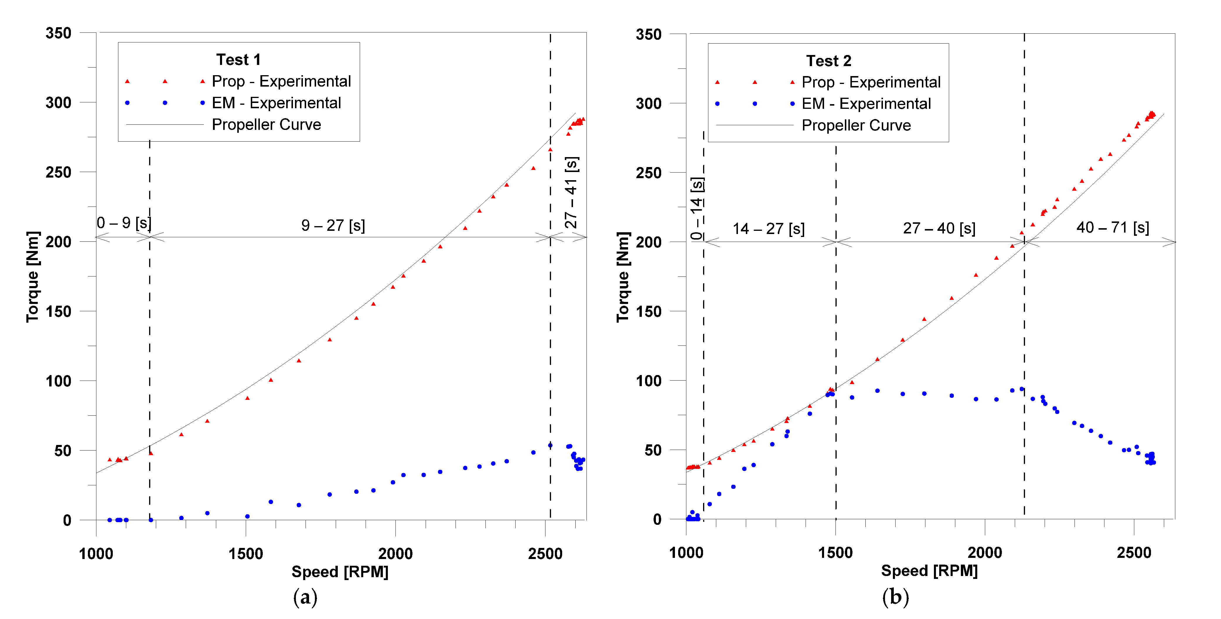
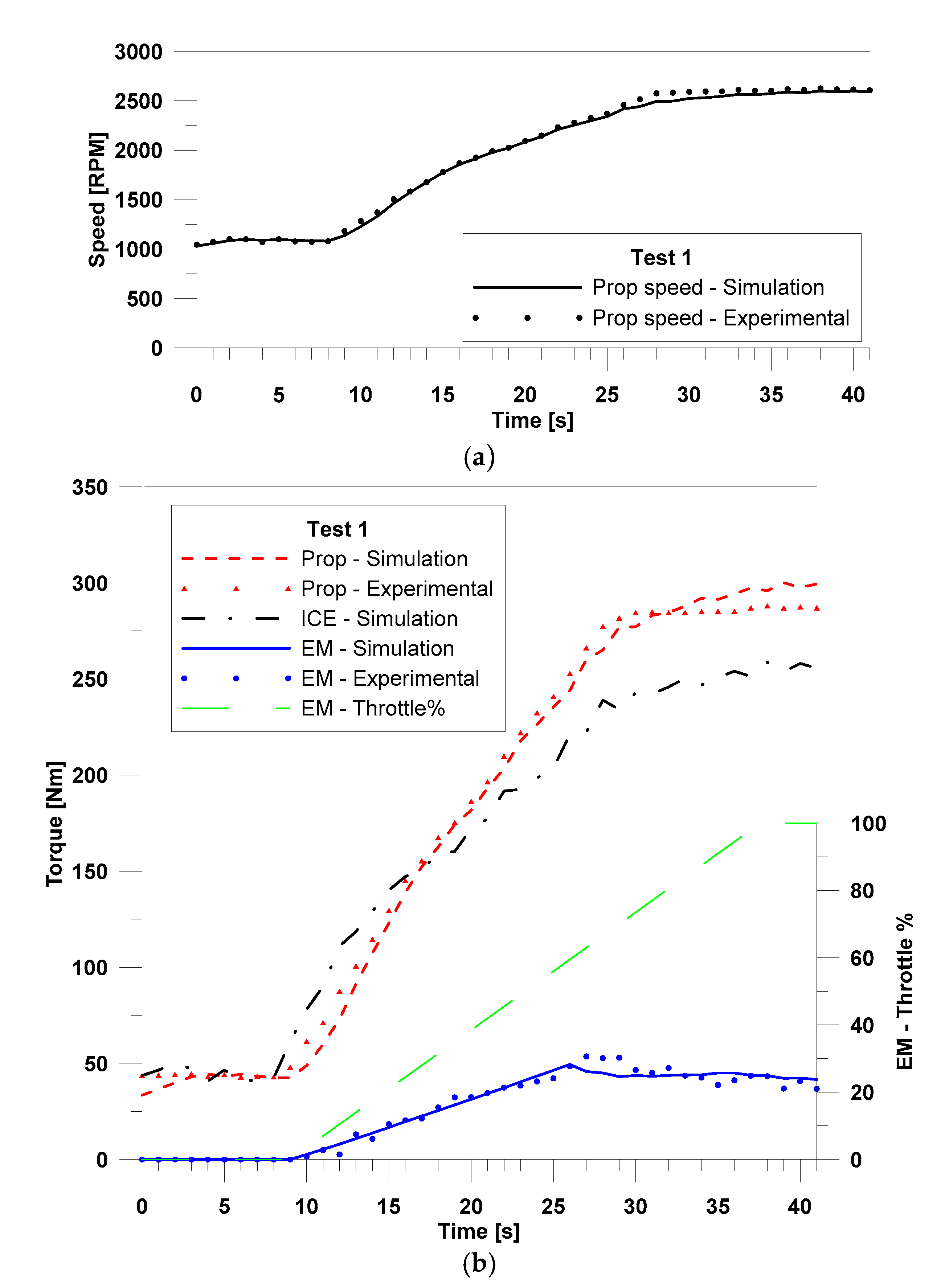
Figure 2a shows the brake and EM experimental torque curves related to the first test (Test 1), which lasted 41 seconds and consisted of two phases:
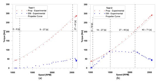
Figure 2.
Experimental tests torque–rotational speed measurements: (a) Test 1; (b) Test 2.
- From t = 0 s to t= 9 s the brake limited the system speed to 1000 RPM, the ICE supplied the power to keep the system at equilibrium while the EM was inactive;
- From t = 9 s to t = 41 s both throttles were raised together to increase the system speed to 2500 RPM. At the speed of 2400 RPM (t = 27 s), the EM started the de-fluxing functioning.
Figure 2b shows the brake and EM experimental torque curves relative to the second test (Test 2), which lasted 72 seconds and consisted of three phases.
- From t = 0 s to t = 14 s the brake limited the system speed to 1000 RPM, the ICE supplied the power to keep the system at equilibrium while the EM was inactive;
- From t = 14 s to t = 27 s the system was accelerated from 1000 RPM to 1500 RPM. In this case, only the EM throttle was raised progressively to 100%, while the ICE was at minimum throttle. The EM throttle reached 100% at t = 26 s;
- From t =27 s to t = 71 s the ICE supplied more torque until the system reached 2500 RPM. The EM de-fluxing functioning started at 2200 RPM (t = 40 s).
2.2. Model Design
The proposed numerical model simulates hybrid electric propulsion systems that have a general scheme close to the one described in the previous paragraph. The freewheel can automatically de-couple the ICE whenever its power is not required. The EM is always coupled with the propeller, and it acts as a motor or generator depending on the power requirements; whenever the EM is not powered, it acts as a flywheel. The proposed numerical model can simulate every described case. In the most complex case (ICE and EM active), the model follows the logic scheme shown in Figure 3.
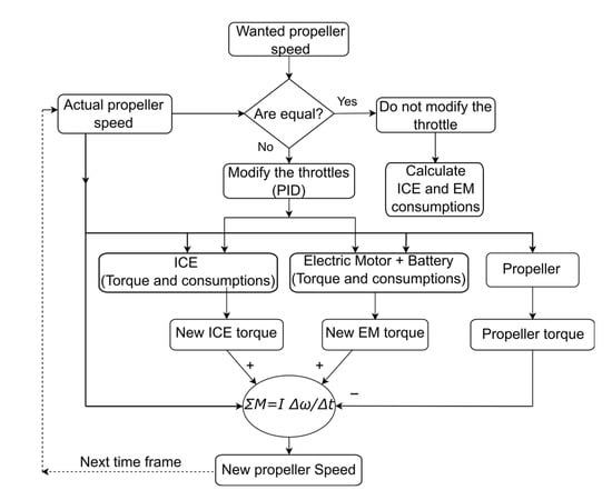
Figure 3.
Model logic scheme.
The model control parameter is propeller speed, which is compared with the propeller speed related to the desired mission. Two PIDs controllers adjust the ICE and EM required torque based on the difference between the calculated propeller speed and the desired one. The net torque (difference between the positive torque and the resistant torque) cause propeller speed variations depending on the system inertia, Equation (1).
where is the ICE torque, is the EM (positive or resistant) torque, is the propeller’s resistant torque at each t instant; is the system’s overall moment of inertia, and is the system’s angular speed variation in the unit time.
The moment of inertia consists of three components (Table 3): was given by the manufacturer’s EM datasheet; in this case, was replaced by the brake dynamometer moment of inertia; the remaining moment of inertia (ICE, pulleys, and free wheel inertia) was obtained through a calibration process and reflected to the propeller shaft.
Table 3.
Moment of inertia.
The ICE and EM PIDs are independent from each other so that they can simulate the actual reactivity of every element.
2.2.1. ICE Model
A simplified model describes the ICE. It cannot consider fluid-dynamic issues. Generally, the ICE torque () is a function of the rotational speed n, altitude H, and throttle position. The manufacturer provides the maximum engine torque as a function of rotational speed at sea level, and a correction map [19] to calculate the engine performance at different altitudes (H) at the International Standard Atmosphere (ISA). The manufacturer does not provide a relationship between torque and throttle position.
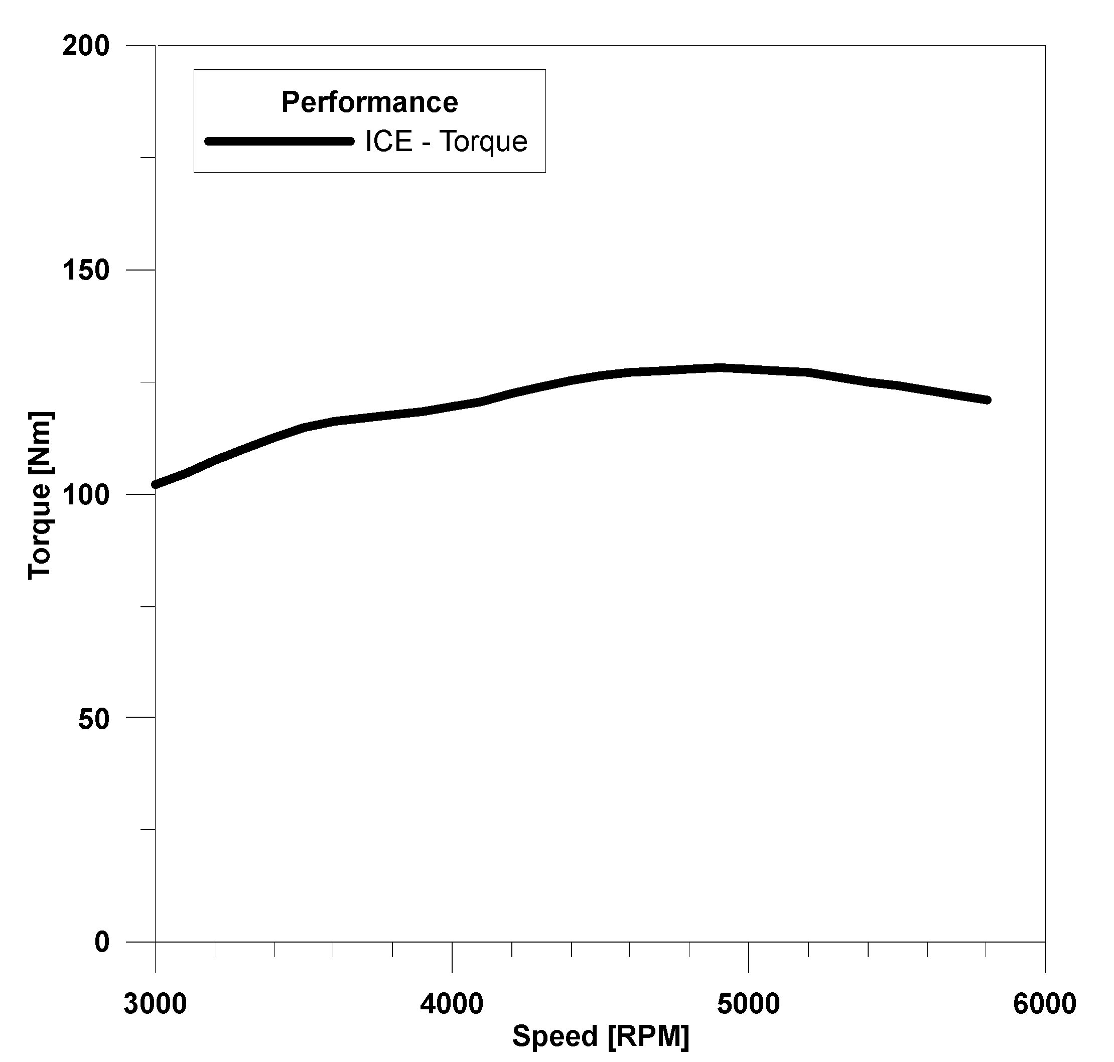
The maximum torque curve (Figure 4) and the correction altitude map is loaded in the model using Look Up Tables (LUT). However, these tests were performed at sea level, so no correction was needed.
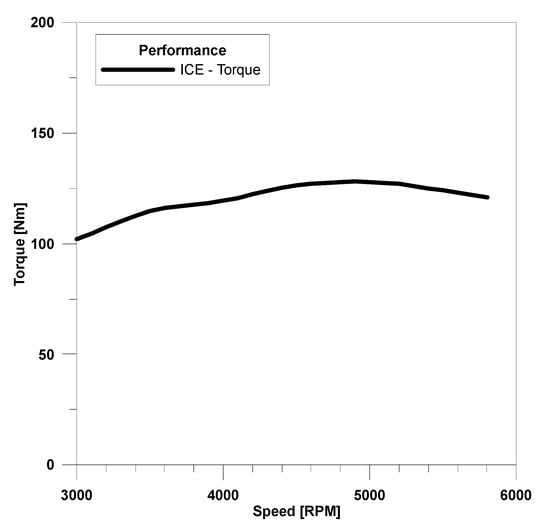
Figure 4.
ICE maximum torque manufacturer’s curve.
The torque’s dependence on the throttle has not been modelled. On the contrary, the PID controller defines (instant by instant) the ICE torque output as a rate (from 0% to 100%) of the maximum available at that instant ICE rotational speed. In this way, there is no relationship between throttle angle position and PID output value.
Finally, the output torque is amplified considering the total transmission ratio .
2.2.2. Battery Model
The Li-ion battery was modelled through an equivalent electric circuit, as also shown by Tremblay and Dessaint [20]. The mathematical relationship used to describe the circuit is shown in Equations (2) and (3).
where is the discharging or charging current, is the filtered current value, is the battery capacity and is the current time integral plus the initial battery charge. , , , , and refer to the actual battery cell’s characteristics or calibration constants. In this study, these constants were set to the typical values proposed by Tremblay and Dessaint [20].
2.2.3. Electric Motor/Generator Model
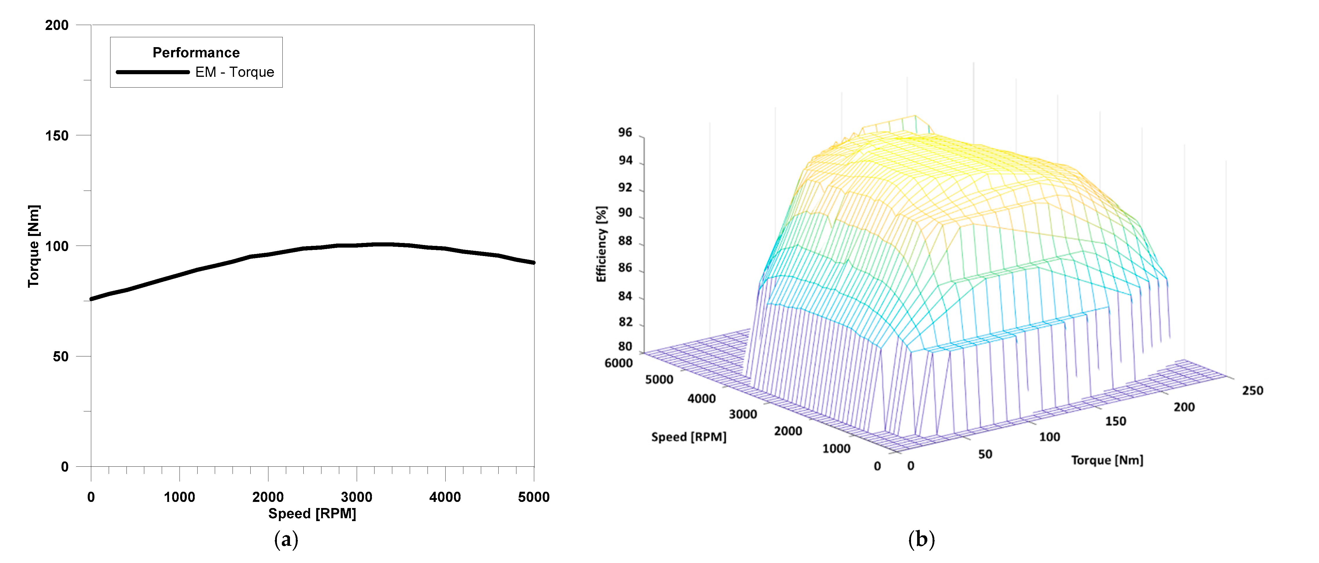
The EM torque curve was also expressed as a LUT. A 2D LUT modelled the EM efficiency as a function of the torque and the rotational speed. Figure 5 shows the graphical representation of these LUTs.

Figure 5.
Manufacturer’s data. (a) EM maximum torque; (b) efficiency map.
The EM and battery models are linked through energy relationships, as the EM model cannot consider electric quantities. Therefore, the EM available torque , at its rotational speed, is converted to a power request to the battery at its available voltage. The power demand is converted to a current demand , based on the battery voltage at the previous instant (t−1), as illustrated in Equation (4).
where the instant (t) battery voltage (Equation (5)) is calculated through Equations (2) and (3).
Finally, the actual torque supplied is calculated based on the instant (t) voltage and current (see Equation (6)).
During ordinary functioning, the difference between and is below 1%. However, this calculation allows the evaluation for each instant of the battery power availability under abnormal conditions, i.e.,
- The charge or discharge current exceeds the battery upper limits;
- The EM is in the de-fluxing function.
In the first case, the model coerces the current value to the battery’s upper limit, so the torque is limited as well (see Equations (4), (5) and (6)).
As for the latter, a dedicated model function simulates this abnormal condition, which occurs every time the ratio between the EM rotational speed and the battery voltage exceeds the EM specific load speed (SLS) value (RPM/Volt) (the EMRAX 228 Low Voltage SLS is 34). So, the model’s de-fluxing function limits the EM torque whenever that ratio exceeds the EM SLS. In this case, the EM needs extra current to perform the flux weakening of the permanent magnets. The model does not consider that current. Its calculation needs further experimental data, or a more complex model coupled with additional manufacturer’s data. However, this approximation is acceptable as this functioning is unwanted.
2.2.4. Propeller Model
The propeller resistive load is modelled by Equation (7). This model does not consider the advance ratio (see Equation (8)), but it is reliable for quasi static translations.
where A, B and C are propeller coefficients, n is the rotational speed expressed in RPM, M is the propeller torque expressed in Nm, J is the advance ratio, is the freestream fluid velocity expressed in m/s, D is the propeller’s diameter expressed in m. Equation (7) parameters values are presented in Table 4.
Table 4.
Propeller curve parameters.
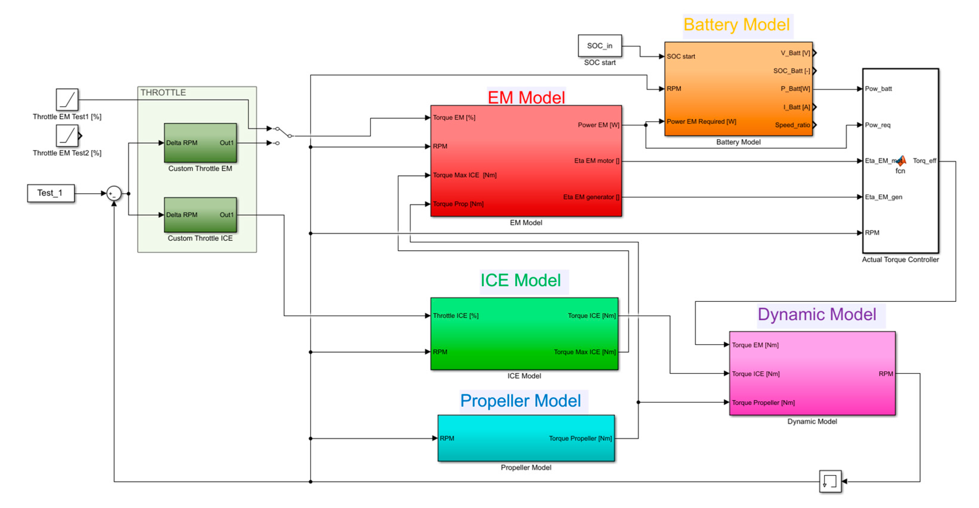
Figure 6 shows the block scheme of the MATLAB® Simulink® overall model.

Figure 6.
Block scheme of the MATLAB Simulink overall model.
3. Results
The model replicates the first test experimental data, handling the ICE throttle through the PID controller while the EM throttle is managed through a predefined function. This function consists of two parts:
- From t = 0 s to t = 9 s the throttle is 0%;
- From t = 9 s to t = 41 s the throttle follows a linear rise (as a function of time) until 100% (see also the green long-dashed line in Figure 7b).
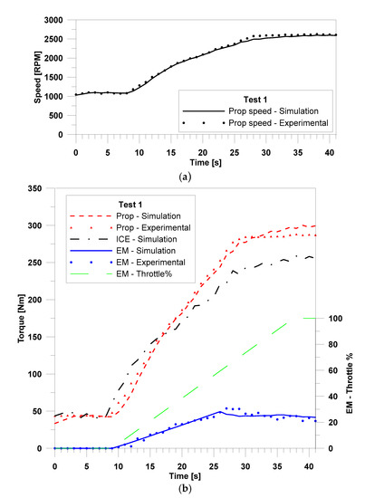 Figure 7. Test (a) experimental and calculated speed curves; (b) experimental and calculated torque curves.
This function describes the actual EM throttle management during the execution of the test 1 experiment.
Figure 7a shows the simulated and experimental propeller speed. Figure 7b shows the propeller-simulated resistant torque, and the EM and ICE-simulated torque. Also, the experimental propeller and EM torque is shown. Table 5 compares the mean error and its standard deviation for the experimental and simulated quantities. As for the EM, only the de-fluxing functioning was taken into consideration.
Table 5.
Test 1 simulation error and error standard deviation.
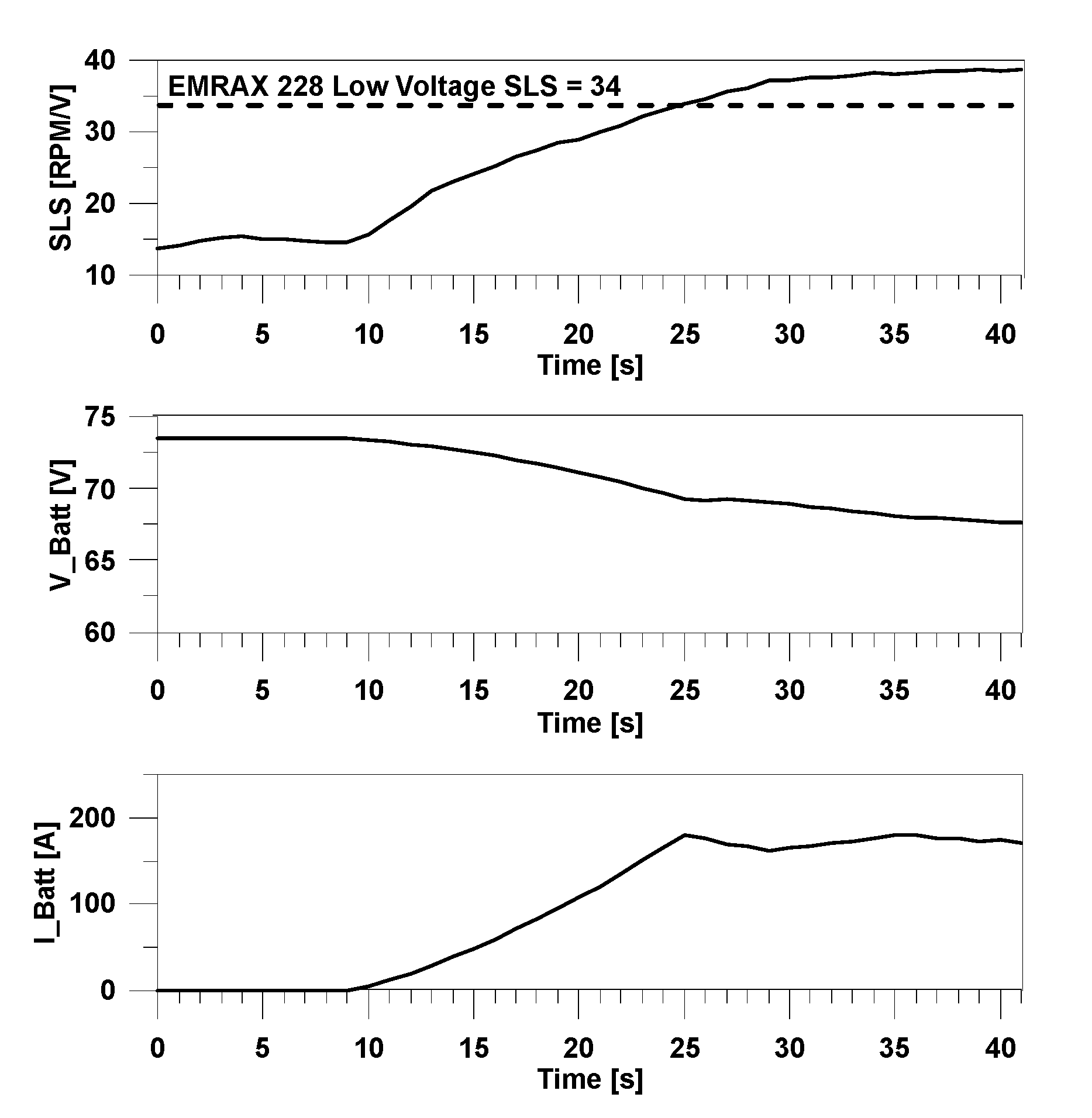
The model estimates the fundamental battery quantities (i.e., instantaneous battery voltage and current) and the instantaneous SLS ratio. This parameter is calculated to switch the model to the de-fluxing functioning case. Whenever it exceeds the SLS maximum value of the EM (in this case at the 26th second), the model limits the battery current as shown in Figure 8.
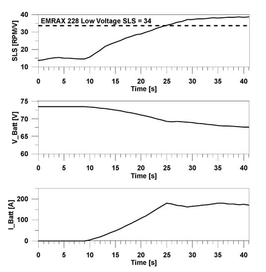
Figure 8.
Test 1: calculated SLS, battery voltage and current.
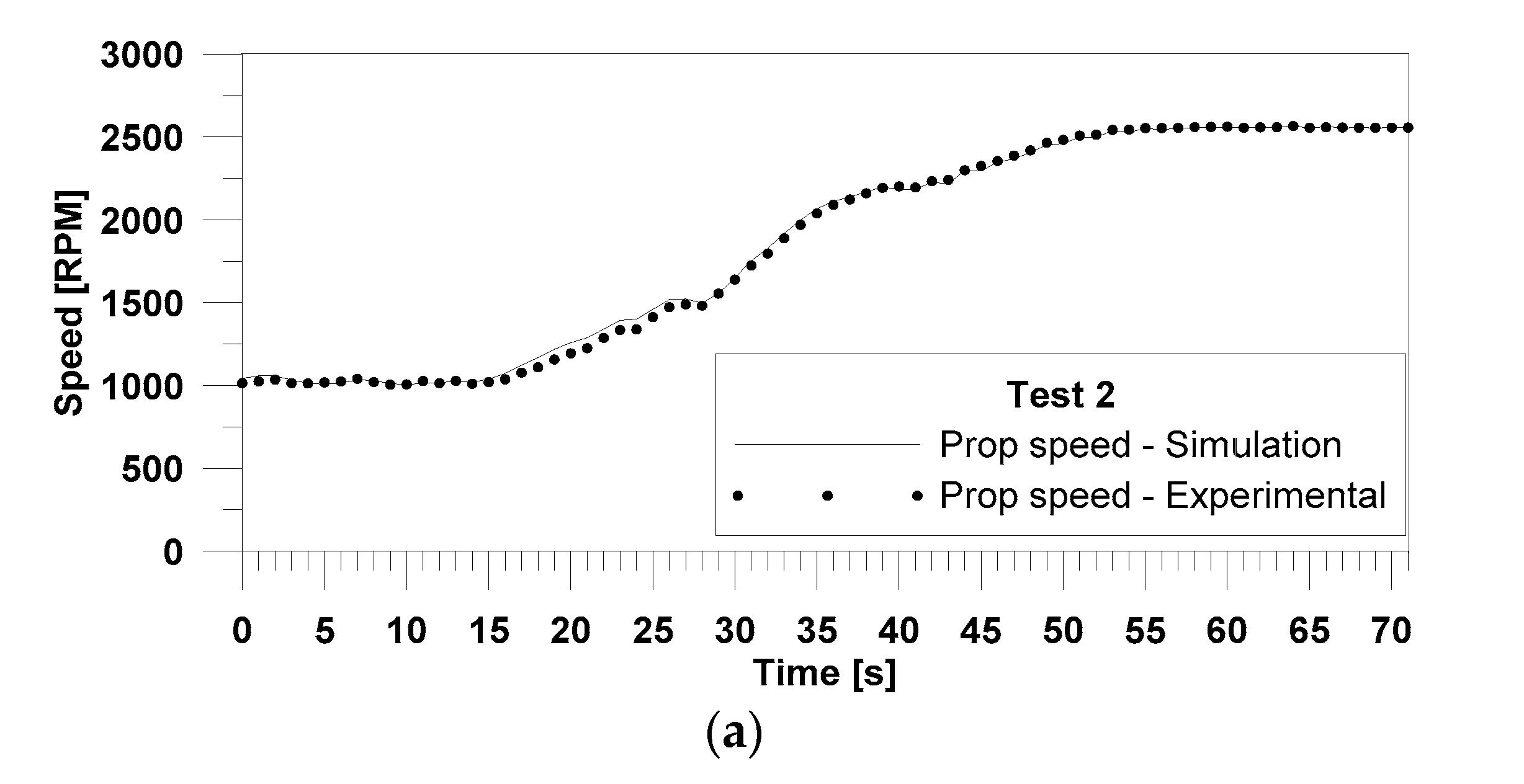
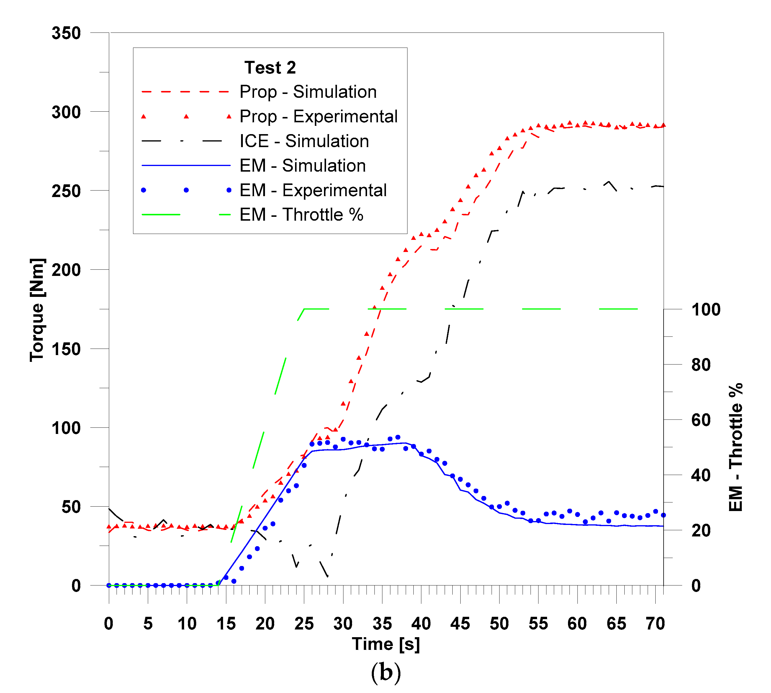
As in the previous case, the model replicated the experimental data. The model ICE throttle was handled by the PID controller and the EM throttle follows a predefined function. This function consists of three parts:
- From t = 0 s to t = 13 s the throttle is 0%;
- From t = 14 s to t = 26 s the throttle follows a linear increase (as a function of time) until 100% (see also green long-dashed line in Figure 9b).
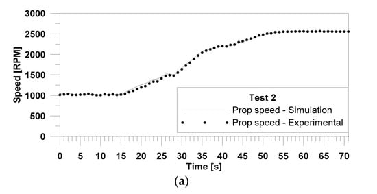
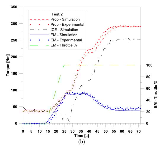 Figure 9. Test 2: (a) experimental and calculated speed curves; (b) experimental and calculated torque curves.
 - From t = 27 s to t = 71 s the throttle is constant at 100%.
Figure 9a shows the simulated and experimental propeller speed. Figure 9b shows the propeller-simulated resistant torque, and the EM and ICE-simulated torque. Also, the experimental propeller and EM torque is shown. Table 6 compares the mean error and its standard deviation for the experimental and simulated quantities. As for the EM, only the de-fluxing functioning was taken into consideration.
Table 6.
Test 2 simulation error and error standard deviation.
Figure 10 shows the instantaneous SLS and battery voltage and current calculated in the Test 2 simulation. In this case, the current limitation (starting from the 40th second) is even more evident than in the Test 1 simulation because the battery voltage reached a lower value.
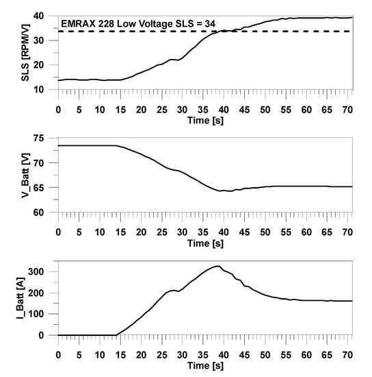
Figure 10.
Test 2: calculated SLS, battery voltage and current.
4. Discussion
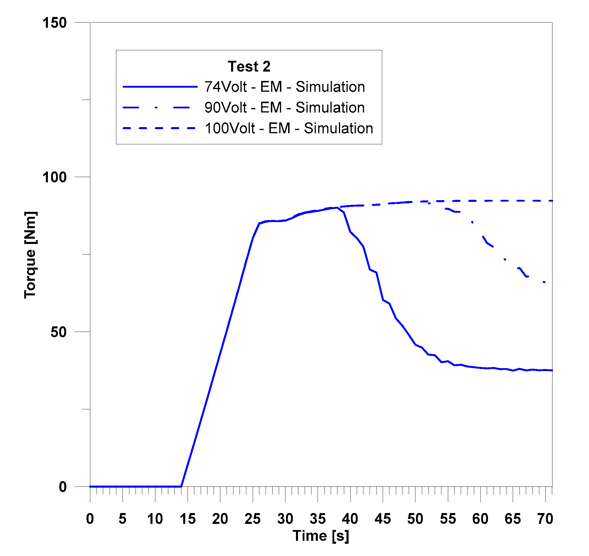
The de-fluxing phenomena shown in tests 1 and 2, are caused by the rapid battery drop voltage at high speed. An investigation into the battery size in order to avoid the de-fluxing phenomena is presented below.
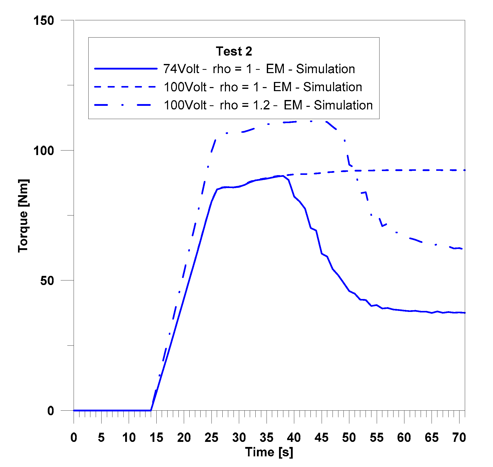
Specifically, test 2 was repeated by increasing the nominal voltage of the battery. At first, the voltage was increased to 90 V and then to 100 V. The nominal capacity and starting SOC did not change (40 Ah and 50%). The results clearly show that if the battery voltage increases, the de-fluxing phenomena decrease (see Figure 11). In fact, at 90 V the de-fluxing phenomena were less evident, and at 100 V they were eliminated. This analysis was conducted leaving the transmission ratio (equal to ) between the EM and brake (propeller) unchanged.

Figure 11.
Comparison between calculated torque curves based on test 2: battery voltage of 74 V, 90 V, 100 V.
Subsequently, an investigation was conducted by changing the transmission ratio, assuming . In this case, the operating points of the EM moved at a higher RPM. Figure 12 shows the torques calculated with a 100 V nominal voltage battery and two different EM gear ratios, and . Figure 12 also shows the case of a 74 V battery and EM gear ratio of . The increased EM speed causes the de-fluxing functioning, even with an increased battery voltage. The EM torque calculated with is higher as every torque refers to the propeller shaft.
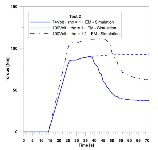
Figure 12.
Comparison between calculated torque curves based on test 2 at different EM gear ratio and battery voltage.
5. Conclusions
The model consistently replicated the results of the experimental tests carried out under abnormal operating conditions. Despite the highly simplified model, the margin of error between the experimental and simulated results was less than 8%.
According to the objective mission, the high versatility and speed of calculation allows a large number of preliminary assessments to be conducted for the identification of the best hybrid architecture (e.g., gear ratio, degree of hybridization), to choose each component (ICE, EM, and battery) and to identify the energy interaction between the components.
The battery model consistently calculates the related quantities, although it has not been validated on the actual battery. Future activities will focus on the electrical quantities measurements to enhance the model and complete the validation.
Future model improvements will involve the ICE partial load simulation. The actual torque will be related to manifold air pressure: this is a more reliable parameter than the throttle position. Moreover, future developments will allow the simulation of different propulsion architectures (e.g., serial and mixed configurations) and interaction with the aircraft model to simulate an entire flight mission.
Author Contributions
The conceptualization, methodology and experimental design were developed by M.C.; the data acquisition system was enhanced by B.G.; the experimental data acquisition was performed by M.C. and E.F.; the data analysis was performed by E.F.; the software model development and model calibration were performed by E.F. and B.G. All authors have read and agreed to the published version of the manuscript.
Funding
This research received no external funding.
Data Availability Statement
Not applicable.
Acknowledgments
The authors would like to thank Salvatore De Cristofaro for his technical assistance.
Conflicts of Interest
The authors declare no conflict of interest.
Nomenclature
Acronyms
| EM | Electric Motor |
| FEPS | Full Electric Propulsion System |
| HEPS | Hybrid Electric Propulsion System |
| ICE | Internal Combustion Engine |
| LUT | Look Up Table |
| PMSM | Permanent Magnet Synchronous Motor |
| RPM | Rotations per Minute |
| SLS | Specific Load Speed |
| SOC | State of Charge |
| UAV | Unmanned Aerial Vehicle |
Physical quantities
| D | Propeller diameter [m] |
| I | Moment of inertia [kg × m2] |
| i | Current [A] |
| J | Advance ratio [-] |
| M | Torque [N*m] |
| n | Rotational speed [RPM] |
| T | Temperature [°C] |
| t | Time [s] |
| V | Voltage [V] |
| v | Fluid speed [m/s] |
| ρ | Transmission ratio [–] |
| ω | Rotational speed [rad/s] |
| Rotational acceleration [rad/s2] |
References
- Agarwal, R. Sustainable (Green) Aviation: Challenges and Opportunities. SAE Int. J. Aerosp. 2009, 2, 1–20. [Google Scholar] [CrossRef]
- Hu, S.; Fruin, S.; Kozawa, K.; Mara, S.; Winer, A.M.; Paulson, S.E. Aircraft Emission Impacts in a Neighborhood Adjacent to a General Aviation Airport in Southern California. Environ. Sci. Technol. 2009, 43, 8039–8045. [Google Scholar] [CrossRef] [PubMed]
- Lee, W.; Kang, M.-Y.; Yoon, J.-H. Cancer Incidence Among Air Transportation Industry Workers Using the National Cohort Study of Korea. Int. J. Environ. Res. Public Health 2019, 16, 2906. [Google Scholar] [CrossRef] [PubMed] [Green Version]
- Xie, Y.; Savvarisal, A.; Tsourdos, A.; Zhang, D.; Gu, J. Review of hybrid electric powered aircraft, its conceptual design and energy management methodologies. Chin. J. Aeronaut. 2021, 34, 432–450. [Google Scholar] [CrossRef]
- Bai, M.; Yang, W.; Song, D.; Kosuda, M.; Szabo, S.; Lipovsky, P.; Kasaei, A. Research on Energy Management of Hybrid Unmanned Aerial Vehicles to Improve Energy-Saving and Emission Reduction Performance. Int. J. Environ. Res. Public Health 2020, 17, 2917. [Google Scholar] [CrossRef] [PubMed] [Green Version]
- Glassock, R.; Galea, M.; Williams, W.; Glesk, T. Hybrid Electric Aircraft Propulsion Case Study for Skydiving Mission. Aerospace 2017, 4, 45. [Google Scholar] [CrossRef]
- Friedrich, C.; Robertson, P.A. Design of Hybrid-Electric Propulsion Systems for Light Aircraft. In Proceedings of the 14th AIAA Aviation Technology, Integration, and Operations Conference, Atlanta, GA, USA, 16–20 June 2014. [Google Scholar]
- Xie, Y.; Savvaris, A.; Tsourdos, A.; Laycock, J.; Farmer, A. Modelling and control of a hybrid electric propulsion system for unmanned aerial vehicles. In Proceedings of the 2018 IEEE Aerospace Conference, Big Sky, MT, USA, 3–10 March 2018; pp. 1–13. [Google Scholar] [CrossRef] [Green Version]
- Sliwinski, J.; Gardi, A.; Marino, M.; Sabatini, R. Hybrid-electric propulsion integration in unmanned aircraft. Energy 2017, 140, 1407–1416. [Google Scholar] [CrossRef]
- Narum, E.F.L.; Hann, R.; Johansen, T.A. Optimal Mission Planning for Fixed-Wing UAVs with Electro-Thermal Icing Protection and Hybrid-Electric Power Systems. In Proceedings of the 2020 International Conference on Unmanned Aircraft Systems (ICUAS), Athens, Greece, 1–4 September 2020; pp. 651–660. [Google Scholar] [CrossRef]
- Sands, T. Development of Deterministic Artificial Intelligence for Unmanned Underwater Vehicles (UUV). J. Mar. Sci. Eng. 2020, 8, 578. [Google Scholar] [CrossRef]
- Bongermino, E.; Mastrorocco, F.; Tomaselli, M.; Monopoli, V.G.; Naso, D. Model and energy management system for a parallel hybrid electric unmanned aerial vehicle. In Proceedings of the 2017 IEEE 26th International Symposium on Industrial Electronics (ISIE), Edinburgh, UK, 19–21 June 2017; pp. 1868–1873. [Google Scholar] [CrossRef]
- Xie, Y.; Savvaris, A.; Tsourdos, A. Fuzzy logic based equivalent consumption optimization of a hybrid electric propulsion system for unmanned aerial vehicles. Aerosp. Sci. Technol. 2019, 85, 13–23. [Google Scholar] [CrossRef] [Green Version]
- Zhang, X.; Liu, L.; Dai, Y. Fuzzy State Machine Energy Management Strategy for Hybrid Electric UAVs with PV/Fuel Cell/Battery Power System. Int. J. Aerosp. Eng. 2018, 2018, 1–16. [Google Scholar] [CrossRef] [Green Version]
- Cameretti, M.C.; Del Pizzo, A.; Di Noia, L.P.; Ferrara, M.; Pascarella, C. Modeling and Investigation of a Turboprop Hybrid Electric Propulsion System. Aerospace 2018, 5, 123. [Google Scholar] [CrossRef] [Green Version]
- Hung, J.; Gonzalez, F. On parallel hybrid-electric propulsion system for unmanned aerial vehicles. Prog. Aerosp. Sci. 2012, 51, 1–17. [Google Scholar] [CrossRef] [Green Version]
- Frosina, E.; Senatore, A.; Palumbo, L.; Di Lorenzo, G.; Pascarella, C. Development of a Lumped Parameter Model for an Aeronautic Hybrid Electric Propulsion System. Aerospace 2018, 5, 105. [Google Scholar] [CrossRef] [Green Version]
- Machado, L.; Matlock, J.; Suleman, A. Experimental evaluation of a hybrid electric propulsion system for small UAVs. Aircr. Eng. Aerosp. Technol. 2019, 92, 727–736. [Google Scholar] [CrossRef]
- (pp. 5–7, Figure 6). Available online: https://rotax-docs.secure.force.com/DocumentsSearch/sfc/servlet.shepherd/version/download/0681H00000EW7xRQAT?asPdf=false (accessed on 22 June 2021).
- Tremblay, O.; Dessaint, L.-A. Experimental Validation of a Battery Dynamic Model for EV Applications. World Electr. Veh. J. 2009, 3, 289–298. [Google Scholar] [CrossRef] [Green Version]


Publisher’s Note: MDPI stays neutral with regard to jurisdictional claims in published maps and institutional affiliations. |
© 2021 by the authors. Licensee MDPI, Basel, Switzerland. This article is an open access article distributed under the terms and conditions of the Creative Commons Attribution (CC BY) license (https://creativecommons.org/licenses/by/4.0/).